| Issue |
A&A
Volume 635, March 2020
|
|
|---|---|---|
| Article Number | A21 | |
| Number of page(s) | 12 | |
| Section | Planets and planetary systems | |
| DOI | https://doi.org/10.1051/0004-6361/201935814 | |
| Published online | 02 March 2020 | |
A new equation of state applied to planetary impacts
I. Models of planetary interiors★
1
Lund Observatory, Department of Astronomy and Theoretical Physics, Lund University,
Box 43,
22100
Lund,
Sweden
e-mail: This email address is being protected from spambots. You need JavaScript enabled to view it.
2
Institute of Theoretical Astrophysics, University of Oslo,
Postboks 1029,
0315
Oslo,
Norway
e-mail: This email address is being protected from spambots. You need JavaScript enabled to view it.
Received:
1
May
2019
Accepted:
14
January
2020
Abstract
We present a new analytical equation of state (EOS), which correctly models high pressure theory and fits well to the experimental data of ɛ-Fe, SiO2, Mg2SiO4, and the Earth. The cold part of the EOS is modeled after the Varpoly EOS. The thermal part is based on a new formalism of the Gruneisen parameter, which improves behavior from earlier models and bridges the gap between elasticity and thermoelasticity. The EOS includes an expanded state model, which allows for the accurate modeling of material vapor curves. The EOS is compared to both the Tillotson EOS and ANEOS model, which are both widely used in planetary impact simulations. The complexity and cost of the EOS is similar to that of the Tillotson EOS, while showing improved behavior in every aspect. The Hugoniot state of shocked silicate material is captured relatively well and our model reproduces vapor curves similar to that of the ANEOS model. To test its viability in hydrodynamical simulations, the EOS was applied to the lunar-forming impact scenario and the results are presented in Paper II and show good agreement with previous work.
Key words: equation of state / planets and satellites: interiors / Moon / planets and satellites: formation / planets and satellites: dynamical evolution and stability / Earth
The code used to make the analysis can be downloaded at https://github.com/robertwissing/EOS.
© ESO 2020
1 Introduction
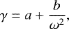
An equation of state (EOS) is used to relate thermodynamical variables, such as temperature, density, and pressure, to each other. The pressure and internal energy of a solid can be described as the sum of the following three parts (Zel’dovich & Raizer 1967): the cold term, which represents the temperature independent interatomic potential, the vibrational part, which represents the vibrations of the atomic lattice, and the electronic term, which represents the thermal excitation of the free electrons. There have been a number of different EOSs developed for solids, many of which are specialized for a certain purpose. Finite strain EOSs describe a material under isothermal conditions (most often at zero degrees). These are often used in the fitting of compression data, where the two most used are the Birch-Murnhagen (B-M) (Birch 1947) and the Vinet EOS (Vinet et al. 1987). At higher temperatures, the effect from lattice vibrations and free electrons becomes significant. These properties are often modeled by using a thermal EOS, such as the Mie-Gruneisen EOS (Mie 1903). When modeling planetary interiors, we require an EOS that gives a realistic description of a material for a wide range of different pressures, temperatures, and states of matter. This includes the capturing of shock states, which are highly important in planetary impacts. This is why more advanced EOSs such as ANEOS (Thompson & Lauson 1972; Melosh 2007) and the Tillotson EOS (Tillotson 1962; Brundage 2013), are often used. ANEOS is a highly complex semi-analytical EOS that has explicit treatment of the different phases of matter. The ANEOS model is, however, more costly than the Tillotson EOS, which is a simple analyical model. This is likely the reason why the Tillotson EOS still remains popular in planetary impact simulations (Citron et al. 2015; Marinova et al. 2008; Reinhardt & Stadel 2017). However, there are severe flaws with the Tillotson EOS, the main one being the lack of a proper vapor transition, which leads to erroneous decompression velocities as shown in Stewart et al. (2019). One of the main goals of this paper is to provide a simple analyical EOS that can capture high pressure behavior together with a correct treatment of the vapor transition to give a more suitable simple alternative to a more complex EOS, such as ANEOS. To succeed in this, we focus on improving the modeling of two of the most important parameters in high pressure theory, the pressure derivative of the bulk modulus (B′) and the Gruneisen parameter (γ). The bulk modulus describes a material’s resistance to uniform compression and the Gruneisen parameter describes how pressure changes with the thermal energy. The foundation of the EOS comes from a paper by Weppner et al. (2015), which presents a new cold EOS derived from the pressure derivative of the bulk modulus and the polytrope method. Where a polytrope is a structural assumption between pressure and density and it is also a solution to the Lane-Emden equation. The polytrope is defined as:
![Mathematical equation: \[P=K\rho^{p_E},\]](/articles/aa/full_html/2020/03/aa35814-19/aa35814-19-eq1.png)
where pE is the polytrope exponent. The authors show that the polytrope exponent is equivalent to the pressure derivative of the bulk modulus,  1. This allows for an implementation of real material variables within the polytrope method. This is done by augmenting the classical Lane-Emden equation to handle zero pressure densities and a variable polytrope exponent. To correctly model the polytrope exponent, Weppner et al. (2015) also present an EOS (the Varpoly EOS) based on a variable polytrope exponent:
 (1)
(1)
![Mathematical equation: \[ \eta=\frac{\rho}{\rho_0}. \]](/articles/aa/full_html/2020/03/aa35814-19/aa35814-19-eq4.png)
The parameters A0, A1, and A2 are connected to the extremes of the polytrope exponent by ambient pressure data and Thomas-Fermi Dirac (TFD) theory (Salpeter 1967). In spite of its simplicity, the EOS provides an improvement in the modeling of P, B, B′ over the other popular finite strain EOS. At extreme pressures, solids are predicted to follow TFD high pressure theory. Within TFD theory the infinite pressure asymptote of the polytrope exponent goes toward  . This is the value that a finite strain EOS should go to, however, the B-M EOS goes toward a higher asymptote of
  and the Vinet EOS, in contrast, goes toward a lower asymptote of
  . The sensitivity to the compression curve with respect to the polytrope exponent is clearly shown in Weppner et al. (2015) and this highlights its importance when dealing with planetary interiors. The Varpoly EOS acts as the cold part of our EOS and in the following sections, we add a temperature dependent term to it. In addition, we develop a new model for the Gruneisen parameter, which is shown to fit well with experimental data and adheres to infinite pressure values. To correctly model the vapor transition, we introduce an expanded state model which can be seen to give good fits to prior estimates of the vapor curve. The EOS is thenfit to experimental data and compared to both the Tillotson EOS and the ANEOS model. We also test its caliber to model planets by fitting it to the Preliminary Reference Earth Model (Dziewonski & Anderson 1981). In the second paper, we perform numerical simulations on the lunar-forming impact, to test its merit in planetary impacts.
In Sects. 2 and 3 we go through the development of the EOS. In Sect. 4 we test the EOS by fitting it to experimental data of ɛ-Fe and comparing it to the Tillotson EOS, and we also take a look at how well the EOS compares to the multiphase ANEOS model, in which we focus on the behavior of silicate material (SiO2, Mg2SiO4). In Sect. 5 we discuss the EOS and our different results and finally end with some conclusions.
2 Adding a temperature dependence
We begin by separating the Helmholtz free energy into three separate parts (Zel’dovich & Raizer 1967).
 (2)
(2)
The indices T0 represents the cold term, vib the vibration term, and el the electronic term. The electronic term regards the effect of the free electrons. This only becomes significant when working with metals at very high temperatures (Zel’dovich & Raizer 1967). While it does have some effect on the high pressure shocks in planetary impacts, it remains a minor part compared to the cold and vibrational terms. Thus in this work, we only include the cold and vibrational terms. Taking the derivative of the free energy with respect to the volume at constant temperature leads to an expression for the pressure:
 (3)
(3)
The cold pressure  is given by the Varpoly EOS. The vibration pressure
  can be given by the Debye model for solids (Debye 1912).
 (4)
(4)
In the Debye model, the crystal lattice is seen as a collection of oscillators with different oscillation modes. For temperatures far above the Debye temperature (θD), all oscillation modes are fully excited and the heat capacity goes to the classic Dulong-Petit value:
 (5)
(5)
As most of the solid material in this work will be above the Debye temperature we will assume this constant value. By holding entropy constant and deriving the full pressure term with density we can get the adiabatic bulk modulus. Subsequently deriving that with the pressure we get the adiabatic polytrope exponent. The energy, pressure, bulk modulus, and polytrope exponent are all given in Appendix A. To complete our thermal model, we need an expression for the Gruneisen parameter γ and its derivatives.
2.1 Gruneisen parameter
The macroscopic definition of the Gruneisen parameter describes how pressure changes with respect to the thermal energy. The microscopic definition of the Gruneisen parameter (Grüneisen 1912), describes how the oscillation modes within the lattice change with volume:
 (6)
(6)
In the quasi-harmonic approximation2 these two definitions are equivalent to each other. This lets us connect the microscopic with the macroscopic. Frequency of acoustic modes are directly related to the speed of sound (ω ∝ cs), which in turn is connected to the bulk modulus and the Poisson ratio (Poirier 2000):
 (7)
(7)
where f(ν) is a function that depends on the Poisson ratio and its pressure derivative, and it is determined from the energy distribution between the differentmodes. Three Gruneisen models derived from using different assumptions can be generalized into one formula (Irvine & Stacey 1975; Burakovsky & Preston 2004):
![Mathematical equation: \begin{equation*}\gamma=\frac{B_{T_0}'/2-1/6-\frac{t}{3}\left[1-P/\left(3B_{T_0}\right)\right]-\left(P/3\right)\frac{\textrm{d} t}{\textrm{d} P}}{1-\frac{2t}{3}\left(P/B_{T_0}\right)}. \end{equation*}](/articles/aa/full_html/2020/03/aa35814-19/aa35814-19-eq16.png) (8)
(8)
A constant t (d t∕d P = 0) represents each of the three models. Slater (1940) ![Mathematical equation: $\left[\gamma_{\textrm{sl}}\;{=}\;\gamma(t\;{=}\;0)\right]$](/articles/aa/full_html/2020/03/aa35814-19/aa35814-19-eq17.png) assumed that the Poisson ratio was independent of compression. Vashchenko & Zubarev (1963)
assumed that the Poisson ratio was independent of compression. Vashchenko & Zubarev (1963) ![Mathematical equation: $\left[\gamma_{\textrm{VZ}}\;{=}\;\gamma(t\;{=}\;2)\right]$](/articles/aa/full_html/2020/03/aa35814-19/aa35814-19-eq18.png) avoided using a lattice vibration model and instead formed their model from the partition function and free volume theory. Dugdale & MacDonald (1953)
avoided using a lattice vibration model and instead formed their model from the partition function and free volume theory. Dugdale & MacDonald (1953) ![Mathematical equation: $\left[\gamma_{\textrm{DM}}\;{=}\;\gamma(t\;{=}\;1)\right]$](/articles/aa/full_html/2020/03/aa35814-19/aa35814-19-eq19.png) formula can be found by assuming one-dimensional motion within the free volume theory. In Burakovsky & Preston (2004) it is shown that many recent studies find that depending on the pressure for a certain material, different t′ s fit better. Low pressure more often fit well with t = 0, while intermediate pressure fit well with t = 1 and high pressure fit well with t = 2. Furthermore from relations between γ and B′ it is shown that the Gruneisen parameter must go to a value of γ∞ = 0.5 as P goes to infinity to conform with TFD theory (Nagara & Nakamura 1985; Petrov 1994). Equation (8) only goes to this value for t = 2.5. This indicates that t is pressure dependent and approaches 2.5 as pressure goes to infinity.
formula can be found by assuming one-dimensional motion within the free volume theory. In Burakovsky & Preston (2004) it is shown that many recent studies find that depending on the pressure for a certain material, different t′ s fit better. Low pressure more often fit well with t = 0, while intermediate pressure fit well with t = 1 and high pressure fit well with t = 2. Furthermore from relations between γ and B′ it is shown that the Gruneisen parameter must go to a value of γ∞ = 0.5 as P goes to infinity to conform with TFD theory (Nagara & Nakamura 1985; Petrov 1994). Equation (8) only goes to this value for t = 2.5. This indicates that t is pressure dependent and approaches 2.5 as pressure goes to infinity.
2.2 The t-model
Following the discussion at the end of the previous section, we suggest the following t dependence on density:
 (9)
(9)
The equation is connected to the extremes of t (tmin and t∞ = 2.5). The tmin and δt are material dependent variables that are fit to experiment data of γ. Tests show that γ and its volume derivatives  and
and  go toward their predicted infinite pressure values3
  (Shanker et al. 2007; Stacey & Davis 2004; Shanker & Singh 2005). The t-model allows us to construct a thermal model that is consistent with low pressure as well as high pressure behaviour. From Eq. (7) it is evident that the t-parameter is connected with the Poisson ratio. At high temperature, the thermal energy becomes equally distributed between the P-mode and the two S-modes
  . Here VP and VS are the velocities of the P-waves and the S-waves, expressing these in terms of elastic moduli and solving for the Gruneisen parameter gives the acoustic gamma (Poirier 2000):
![Mathematical equation: \begin{equation*}\gamma_A=\gamma_{\textrm{sl}}-\left[\frac{4-5\nu}{(1+\nu)(1-\nu)(1-2\nu)}\right]\frac{\rho}{3}\frac{\textrm{d}\nu}{\textrm{d}\rho}. \end{equation*}](/articles/aa/full_html/2020/03/aa35814-19/aa35814-19-eq25.png) (10)
(10)
Relating Eqs. (8) and (10) gives an ODE for the temperature independent part of ν which can be solved numerically. This connection between γ and ν allows us to construct models that are consistent with both γ data as well as ν data. This is especially useful when trying to determine material parameters from seismic data, as the Poisson ratio can be used to further restrict the parameter space of γ and its derivatives. The Poisson ratio generally increases with pressure and goes toward a value of 0.5.
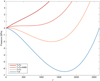 |
Fig. 1 Isothermal expansion curve for α-quartz at different temperatures. The integral over the cold compression curve (blue) is equal to Evap. The minimum of the curve represents a point of instability. As we increase the temperature, we eventually reach the critical isotherm in which the minimum disappears. The critical point represents the point on the critical isotherm, in which the derivative goes to zero. Below the critical temperature the sinusoidal part of the curve is replaced by a constant vapor pressure using Maxwell construction. |
3 Expanded states (ρ < ρ0)
The EOS laid out in the previous section regards solids in compression ρ ≥ ρ0. To get a full description of the material over the whole density range we require a model for the expanded state (ρ < ρ0). During expansion there will be an inward force acting to restore equilibrium. This force will reach a maximum at a certain point. Beyond this point, the intermolecular forces between the atoms start to fade and we begin to move toward the ideal gas case in which there are no intermolecular forces. The energy to separate the atoms from one another will then simply be:
 (11)
(11)
This represents the energy of vaporization or sublimation. The cold pressure in this region will be directed inward (negative). At ρ = ρ0 and ρ = 0 the pressure must go to zero as the first represents the equilibrium point of the solid/liquid and the second represents the ideal gas state. We will as in the extension of ANEOS by Melosh (2007) define the pressure of this region as (Mie 1903):
 (12)
(12)
We require that the bulk modulus is continuous at ρ0, which determines the constant C. The aexp constant is determined from the energy of complete vaporization using Eq. (11). The constant bexp is taken to be a constant and is determined from the dominant intermolecular force (bexp is in the range 1.2–3). We will, as in Melosh (2007), choose a value of bexp = 5∕3, however, bexp can also be set such that the derivative of the bulk modulus remains continuous. For α-quartz this creates the cold expansion curve seen in Fig. 1. This curve represents the phase transition between the compressed state and the vapor state, however, during phase transition, the pressure should remain constant while the material goes from boiling to fully evaporated (or vice versa), using Maxwell construction4 we can replace the sinusoidal part of the curve with a constant vapor pressure. The vapor pressure and density range of this transition will depend on the vapor curve which is generated from the Maxwell construction over a wide range of temperatures (see Sect. 4.4). At a high enough temperature, we eventually reach a temperature in which the sinusoidal part of the curve disappears (see Fig. 1). This is the critical isotherm, the point at which its derivative goes to zero represents the critical point, where the distinct phase transition between liquid and gas vanish. The critical point will depend on the cold minimum and the behavior of the Gruneisen parameter and the heat capacity in the expanded state. As our formulation of the Gruneisen parameter is only valid in the compressed states, we require a new formulation for the expanded state, namely
 (13)
(13)
 (14)
(14)
![Mathematical equation: \[ \gamma_k=1+\gamma_0-\gamma_{\textrm{ideal}}. \]](/articles/aa/full_html/2020/03/aa35814-19/aa35814-19-eq30.png)
This is an empirical fitting formula that ensures that the Gruneisen parameter and its volume derivative are continuous at ρ0 and that it conforms to the ideal gas law at zero density. The constant dexp is fit so that q goes to q0 at ρ0 :
![Mathematical equation: \[ d_{\textrm{exp}}=q_0\gamma_0+c_{\textrm{exp}}\gamma_k, \]](/articles/aa/full_html/2020/03/aa35814-19/aa35814-19-eq31.png)
and cexp can be determined by either the materials critical point temperature (if known) or the boiling temperature at 1 bar, or if not available it can be set to around cexp = 0.6 ↔ 1.0. The heat capacity remains constant and the same as in the compressed state, which forces a lower Gruneisen parameter at the zero density limit to capture the correct ideal gas pressure.
![Mathematical equation: \[ \begin{array}{l} \gamma_{\textrm{ideal}}=\frac{1}{3}, \\[4pt] C_v=3Nk. \end{array} \]](/articles/aa/full_html/2020/03/aa35814-19/aa35814-19-eq32.png)
The expanded state model is tested in detail and compared to the ANEOS model in Sect. 4.4. A full description of the model can be viewed in Appendices B and C.
4 Testing
In this section, the EOS is tested against different kinds of experimental data and compared to the Tillotson EOS and the ANEOS model. In the first subsection, we fit our EOS to the cold compression curve and the Gruneisen parameter of ɛ-Fe. In the second subsection, we perform a fit to the Preliminary Reference Earth Model (PREM; Dziewonski & Anderson 1981). In the third subsection, we fit our model to the experimental Hugoniot curve for iron and compare our model to the Tillotson EOS. In the fourth subsection, we compare our EOS to the ANEOS model and perform fits to the Hugoniot curve of silicates and their respective vapor curves. For the iron related results, we perform three fits which are named “Fit to Compression, PREM, and Hugoniot” respectively. For the silicate related results, we perform two fits which are named “Fit to quartz/forsterite data” and “Fit to Hugoniot”.
4.1 Fitting to ɛ-Fe data
At pressuresabove 16 GPa, α-Fe changes phase to ɛ-Fe (see Fig. 2) making it the most abundant phase of iron in planetary interiors. The material properties ( ) of ɛ-Fe are determined from high pressure compression data (Dewaele et al. 2006). Here the compression curve (P,V) was measured in quasi-hydrostatic conditions up to 205 GPa at 298K using a diamond anvil method. ρ0 is determined from low-pressure measurements, B0 can be set to its value from ultrasonic experiment B0 = 165 GPa.
  is then fit to the experimental compression data using the Varpoly EOS. The fit curve can be seen in Fig. 2 which correspond to
  . In Dewaele et al. (2006) they use the B-M and Vinet EOS instead. Using B-M they got
  and using Vinet
  .
.
For fitting of the Gruneisen parameter, we use data from Anderson (2007) and Anderson & Isaak (2003) that measured how the intensity of X-ray diffraction lines for ɛ-Fe changed under pressure. This data can then be related to the mean square amplitude of the atomic displacement, which in the Debye model relates to the Debye temperature θD (Willis & Pryor 1975). From simultaneous volume data of the sample, they can then extract the Gruneisen parameter. We fit the data to the t-model together with the Varpoly EOS using the material properties from the compression curve fit. The fit curve is seen in Fig. 3 which correspond to tmin = 1.94, δt = 3.89 which correlates toγ0 = 1.76, q0 = 0.86.
A huge benefit of the t-model is that it allows us to correlate the Gruneisen parameter fit with the Poisson ratio, using the acoustic approximation (Eq. (10)). This can then be compared to experimental data of the Poisson ratio which can strengthen the fit and the model. We use an ambient Poisson ratio of ν0 = 0.26 for ɛ-Fe. The calculated Poisson ratio curve is compared to experimental data from Murphy et al. (2013) and can be seen in Fig. 4.
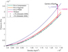 |
Fig. 2 Compression curves of the different models and fits. The green line has been fit to the
ɛ-Fe data from Dewaele et al. (2006) using the Varpoly EOS ( |

4.2 Fitting to the PREM model
The PREM model is a one-dimensional density model of the Earth, constructed from experimental data, gathered using a combinationof methods (Dziewonski & Anderson 1981; Panning & Romanowicz 2006). This model divides up the Earth into nine homogeneous material layers. However, as this includes three quite small layers, we simplify it to six layers. From the center of the planet, these are: the inner core, outer core, lower mantle, transition zone, asthenosphere (low velocity + lid zone), and crust (upper crust, lower crust, and ocean layer). The density of the inner core derived from the PREM model suggests that the inner core mostly consists of iron with small amounts of lighter materials. What lighter material the core consists of is still highly debated (Fischer 2016). For the outer core, the measured S-wave velocities drop to zero. This is indicative of a fluid, which intrinsically has a zero shear-modulus. This has been identified as a molten iron and nickel layer. Between the outer core and the lower mantle lies the core mantle boundary and acts as a thermal boundary layer in which the temperature drops by about 1000 degrees. The lower mantle mostly consists of high pressure materials such as silicate perovskites [(Mg,Fe)SiO3] together with ferropericlases [(Mg,Fe)O]. The transition zone and asthenosphere mostly consists of olivine [(Mg,Fe)2SiO4] which is thelower pressure form of the silicate perovskites. Finally, we have the crust which is very stiff and inhibits large heterogeneities and thus consists of a wide array of different minerals. However, averages of these materials can be taken to give sufficiently good large-scale models. The crust also involves a temperature drop by around 1000 K, which is due to heat loss from conduction. To construct the PREM model, we use a modified version of the method prescribed in Weppner et al. (2015). In which we have added our EOS and an adiabatic temperaturegradient. These modifications add three extra parameters to the material setup, a central temperature TC and the t-model parameters δt and tmin. To fit our density profile to the PREM model, we implement a two-step fitting. We begin by setting up upper and lower boundaries on the material properties ( ). These are determined by the most common minerals of each material layer (Stixrude & Lithgow-Bertelloni 2005) and from the PREM model parameters of Weppner et al. (2015). We decided to determine the thermodynamical parameters tmin, δt from literature values of γ0, q0, as these are often readily available (Dubrovinsky et al. 2000; Stixrude & Lithgow-Bertelloni 2005) and did in the case of ɛ-Fe correlate quite well with experimental data (blue line Fig. 3). The central pressure is taken to be PC = 364.1 GPa which is given in Weppner et al. (2015), we also choose to use the same thickness of each material layer as they do. To correctly model the temperature jump at the core-mantle boundary and the crust we reduce the temperature by around 1000 K between these layers. An initial guess is first made on the central temperature TC. We then begin fitting the density profile to the PREM data. After a fit we readjust the thermodynamical parameters (as these have changed due to new isothermal parameters), we also readjust the central temperature to fit with the approximate melting point (using Lindeman’s law, Gilvarry 1956) of the solid and molten core boundary. We iterate this until convergence. The result of the fit can be seen in Fig. 5 and the material properties of each layer in Table 1. We compute the Poisson ratio for the lower mantle (fitting best with ν0 = 0.255) and the outer core (fitting best with ν0 = 0.4) and compare them to experimental data in Figs. 4 and 6. We can see that the Poisson ratio fits the data from the lower mantle well, however, there is some curvature in the experimental data that is not accounted for. For the Poisson ratio to fit well with the inner core we require a very unlikely high ambient value for it. As the core is mostly made out of iron it should have an ambient Poisson ratio that is much closer to the ɛ-Fe. This mismatch from ɛ-Fe have been studied extensively before (Prescher et al. 2015; Wu 2016) and is thought to either occur from shear softening, carbon alloying, partial melting or high temperature effects. Adding a temperature dependence to the Poisson ratio might improve its behavior, however, we leave this to be the subject for future work.
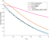 |
Fig. 3 Variation of the Gruneisen parameter with density for the different models and fits. The green line has been fit to experimental data from Anderson (2007) and Anderson & Isaak (2003) using our EOS with tmin = 1.94, δt = 3.89. The PREM curve was fit to ambient pressure values for ɛ-Fe given in Dubrovinsky et al. (2000) (γ0 = 1.78 q0 = 0.69). The Gruneisen parameter from the Tillotson EOS can be seen to have a completely different behavior than the rest. |
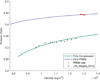 |
Fig. 4 Poisson ratio curve of the compression fit and the PREM fit. The compression fit correlates excellent with the ɛ-Fe data from Murphy et al. (2013). To fit with the PREM data the PREM fit requires an unrealisticly high ambient Poisson ratio of ν0 = 0.4. This is mostlikely due to missing temperature dependent terms of the Poisson ratio for the PREM fit. |
Layers and material properties of our Earth model.
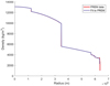 |
Fig. 5 Density model of Earth. Comparison between PREM and our fit. Material parameters for each layer is given in Table 1. |
4.3 Comparison with the Tillotson EOS
The Tillotson EOS was developed for hypervelocity impacts of metals and has been readily used in planetary impacts. Pressure is given by thedensity and internal energy and the EOS includes separate regions for compression and expansion. The region of compression is seen as one continuous phase of matter, while the state in expansion depends on the internal energy. In this section we compare the Tillotson EOS for iron with our EOS in the region of compression.
 (15)
(15)
![Mathematical equation: \[ \omega\;{=}\;\frac{u}{u_0\eta^2}+1. \]](/articles/aa/full_html/2020/03/aa35814-19/aa35814-19-eq40.png)
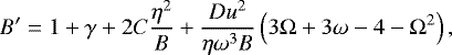
The constant’s a and b are connected to ambient and high temperature constraints of the Gruneisen parameter γ0 = a + b, γT∞ = a. The high temperature constraint is taken to conform with the free electron gas from the TF model (Zel’dovich & Raizer 1967). This is often misinterpreted, it importantly does not mean that the Tillotson EOS correctly extrapolate to the high pressure TFD theory. This can clearly be seen by calculating the polytrope exponent and the Gruneisen parameter:
 (16)
(16)
 (17)
(17)
![Mathematical equation: \[ D=\frac{2b\rho_0}{u_0}, \quad \Omega=\frac{P}{u\rho}, \]](/articles/aa/full_html/2020/03/aa35814-19/aa35814-19-eq43.png)
 (18)
(18)
From this we can see that the Gruneisen parameter will at infinite pressure go back to its ambient pressure value, which is not in correlation with TFD theory. This means that the Gruneisen parameter will decrease at first, until it reaches a minimum (connected to the fitted u0 constant), it will then eventually increase back to its ambient pressure value. The two remaining constant’s C and u0 are fit to experimental Hugoniot data, which describes the locus of the final shock states. For this comparison, we decided to refit the Tillotson parameters for iron as these no longer fit well with more recent high pressure shock data (Brown et al. 2000), the fit parameters can be seen in Table 2.
We also perform a fit with our EOS using the same ρ0, B0 as the Tillotson fit, which can be seen in Table 3. The two fitted Hugoniot curves can be seen in Fig. 7, both fit very neatly to the experimental data. However, the two fit’s does not correlate well with the experimental compression curve of Fig. 2. This will naturally be the case, as we fit a one-phase EOS to the Hugoniot curve which goes through several different phase changes. Starting as α-Fe until about 16 GPa where it changes to ɛ-Fe, then going on to eventually melt at around 150–170 GPa5. The main difference between the Hugoniot fit of our EOS and the Tillotson EOS comes from the cold pressure profiles of its polytrope exponent and Gruneisen parameter. In Fig. 8 we can see that the Tillotson EOS starts to deviate from the other models at around 1 TPa, and goes toward the  from Eq. (18). It is debatable if such high cold pressures would occur in the lunar-forming impact, however, in larger planetary collisions, these pressures are well within reach. In Fig. 3 we can see that the Gruneisen parameter for the Tillotson EOS, behaves very differently than the rest of the models and completely misses the experimental data. The Tillotson EOS cannot distinguish between high temperature behavior and low temperature behavior in this case and models the Gruneisen parameter as seen in highly ionized metals. This will effectively overestimate the thermal pressure and heating for compressed material that is not highly ionized. Another improvement in our EOS is that the transition to the vapor phase is handled better by our model as the latent heat loss due to vaporization or sublimation can be set directly. The Tillotson EOS also does not have a clearrelationship between internal energy and temperature, making it difficult to correctly extract the temperature.
The compression curve in Fig. 2 also highlights another problem, regarding the initial conditions for planets. To reproduce the density and pressure for Earth’s inner core we require a core temperature of around 14 000 K for the compression fit, Hugoniot fit, and the Tillotson EOS. Which is far too high and will result in a planet that is almost fully melted. This can then easily lead to an overproduction of vapor during impact simulations. This also pertains to ANEOS which usually has high initial temperature profiles (as discussed by Barr 2016). This problem mostly originates from trying to fit pure iron to the Earth’s core material, which is an iron alloy. In this paper, we suggest using the fitted PREM model for the inner regions to give a more realistic pressure, density and temperature profile.
Hugoniot fit for iron with Tillotson EOS.
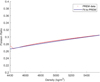 |
Fig. 6 Poisson ratio curve of the lower mantle. We can see that our PREM fit correlates well with the PREM data. The small discrepancy seen at 4400 kg m−3 is due to the transition from the previous planetary layer. |
Hugoniot fit for iron with our EOS.
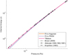 |
Fig. 7 Comparison of the different models to experimental Hugoniot data (Brown et al. 2000; Al’Tshuler et al. 1981; Krupnikov et al. 1963). The Hugoniot fit and the Tillotson fit correlate excellent with the experimental data. Surprisingly the PREM fit correlates well with the experimental data as well. |
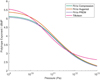 |
Fig. 8 Variation of the polytrope exponent with pressure. All of our EOS fits go to the predicted high pressure value. The Tillotson EOS however diverges around 1012 Pa and goes toward a higher asymptote |
4.4 Comparison with the ANEOS model
The ANEOS model (Thompson & Lauson 1972) is a complex multiphase semi-analytical EOS that includes vapor transition, high temperature behavior, melt transition, mixed states, solid-solid phase changes, etc. In this section, we compare the shock data and vapor curves of quartz and forsterite to the ANEOS model. Both quartz and forsterite are challenging materials to model due to large density changes during high pressure phase changes (quartz-stishovite), the molecular gas behavior and the complicated behavior of the silicate melt (Mosenfelder et al. 2009). As the ANEOSresults presented in this section show data from a wide range of different ANEOS versions, we will describe them shortly. The Melosh (2007) ANEOS version introduced a method to model molecular gas within ANEOS and generally improved the expanded state region. This version seems to be the most used (Nakajima & Stevenson 2014; Canup et al. 2013; Canup 2012; Ćuk & Stewart 2012), which models one high pressure solid–solid phase transition6 but is then unable to accurately model the melt curve. In Collins & Melosh (2014) they improve this method by adding a mixed phase transition for the liquid–solid while retaining the solid–solid phase transition. However, in the ANEOS model the liquid properties are inherently dependent on the underlying solid properties, which has the undesirable effect of giving the melt different properties depending on if it has a cold pressure which is above or below the solid–solid phase transition. In the most recent ANEOS version (Stewart et al. 2019) the high pressure phase change is abandoned in favor of a more accurate melt transition and liquid properties.
We fit the EOS to two different kinds of experimental data. For the first quartz fit, we take zero pressure material properties from Calderon et al. (2007) and Melosh (2007) and for the second quartz fit, we try to fit our material to the experimental Hugoniot curve. For the first forsterite fit, we take material data of olivine from Stixrude & Lithgow-Bertelloni (2005) which is used as our lower mantle material in Paper II (replacing the transition zone, asthenosphere, and crust from Table 1). For the second forsterite fit, we try to fit our material to the experimental Hugoniot curve. As the critical point for any silicate composition has not been experimentally measured, the range of critical parameters (Tc, ρc, Pc) remains highly uncertain. This is why the more experimentally available boiling temperature, vapor and liquid entropies at 1 bar are used to fit the EOS. We set the reference entropy such that the vapor entropy fits roughly the experimental value at 1 bar. For the expanded state EOS we initially use the energy of vaporization from Melosh (2007) to get the cold curve and from the experimental boiling point, we determine the constant cexp which determine the behavior of the Gruneisen parameter in the expanded state. To get a better fit to the vapor curve we additionally allow for small modifications to the energy of vaporization (remains around 1.25 × 10¹¹ erg g−1).
The material parameters are shown in Tables 4 (quartz) and 6 (forsterite). As the critical point for any silicate composition has not been experimentally measured, the range of critical parameters (Tc, ρc, Pc) remains highly uncertain. This is why the more experimentally available boiling temperature, vapor and liquid entropies at 1 bar are used to fit the EOS. We set the reference entropy such that the liquid entropy fits roughly the experimental value at 1 bar. The result of our Hugoniot curves can be seen in Fig. 9 for forsterite and Fig. 10 for quartz. The fit Hugoniot curve of our model can be seen to fit both silicate materials quite well, with quartz being the more difficult case as it exhibits a strong curvature change due to high pressure phase change. This is very difficult for our one-phase model to capture correctly. For the fits to compression data we can see that both quartz and forsterite7 overestimate the pressure after around 100 GPa, this is likely due to not modeling the melt, which occurs around 100 GPa for both material and would cause a lowering of the bulk modulus. This is why the Hugoniot fits always require a smaller bulk modulus to fit the Hugoniot curve, however, the issue with this is that the cold compression curve is not as accurately captured for the Hugoniot fit (see Fig. 12).
The lack of melt is also very related to the failure of capturing the experimental temperature behavior of the Hugoniot in our model. This has been a previous issue for ANEOS but has recently been remedied in the Stewart et al. (2019) version of ANEOS, in which more accurate capturing of the melt together with a higher heat capacity limit (heat capacity in liquid silicate can reach up to Cv = 5NR) allow for accurate fitting to the experimental data. The Tillotson EOS in Fig. 9 can be seen to capture the range [0–200 GPa] relatively well but quickly diverges from the experimental value beyond that. The result of our vapor curve fits can be seen in Fig. 11 and the resulting critical point parameters are tabulated in Tables 5 (quartz) and 7 (forsterite). In addition, we present the Arrhenius plot of forsterite and its temperature vs. density vapor curve in Appendix C, together with an explanation on how vapor pressure is calculated for material within a hydrocode. The two fits are able to fit the boiling temperature and vapor+liquid entropies very well for both materials. As the uncertainty of critical parameters is quite high all fits can be seen to lie within the range of previous estimates. However, for quartz the Hugoniot fit lies in a quite low critical parameter space in which few other estimates are located. For forsterite, we found that the ANEOS fit from Collins & Melosh (2014) does not capture the liquid and vapor entropies well and exhibits a very high critical pressure estimate. It is interesting to note that a simple model of varying the Gruneisen parameter in the expanded state can show similar vapor curves to that of ANEOS with molecular gas behavior, which demonstrates the importance and potential of modeling the Gruneisen parameter.
Quartz material parameters.
Quartz critical point parameters, estimate ranges are from Connolly (2016) and Melosh (2007).
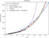 |
Fig. 9 Hugoniot curve for the different fits compared to the results from ANEOS (Stewart et al. 2019). The forsterite experimental data does not exhibit a sharp change as seen in the quartz data and here capturing the melt phase plays a larger role. Both ANEOS and our fit to the Hugoniot conform well with the data, while the fit to the quartz data over pressurizes within the range in which the material has melted (above 100 GPa). We also decided to plot the Tillotson EOS curve for olivine (Marinova et al. 2011), which diverges strongly from the experimental data after around 200 GPa. The experimental data is from Mosenfelder et al. (2007) and Root et al. (2018). |
Forsterite material parameters.
Forsterite critical point parameters, estimate ranges are from Xiao & Stixrude (2018) and Connolly (2016) and experimental entropy estimate from Ahrens & O’Keefe (1972).
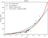 |
Fig. 10 Hugoniot curve for the different fits compared to the results from ANEOS (Collins & Melosh 2014). The experimental data show a sharp change at around
|

5 Conclusions
In this paper we have developed a new analytical equation of state using a free energy expression. The cold part of our EOS was modeled after the Varpoly EOS which has been shown to perform better than other finite strain EOS in accordance with high pressure theory. The thermal part of the EOS was modeled using the Debye model together with the introduction of the t-model. The t-model models the density dependence of the t-parameter within the generalized Gruneisen parameter, which has been indicated to be the case from experiments and high pressure theory. In addition, the connection between the t-parameter and the Poisson ratio bridges the gap between elasticity and thermoelasticity allowing us to check the fitting parameters in terms of one another. The EOS was shown to perform well in reproducing the compression curve, Gruneisen parameter, Hugoniot curve and the Poisson ratio for ɛ-Fe. The Preliminary Reference Earth Model could be modeled well with our EOS, which demonstrates its potential in modeling planetary interiors. Using pure materials compared to derived planetary material was seen to result in unrealistically high central temperatures, so we caution the use of pure materials in favor of derived planetary materials. For the silicates quartz and forsterite, we could see that the model captured the Hugoniot curves relatively well, while also being able to model vapor curves very similar to that of the ANEOS model. There is still much future work to be done to the model (melt, electronic terms, high pressure phases, and heat capacity variations) for it to improve on the behavior of a multiphase EOS such as ANEOS. However, the paper clearly shows that it can act as a suitable and simpler version of ANEOS. The EOS is a significant improvement over the Tillotson EOS that is still widely used in planetary impact simulations. We discourage the use of the Tillotson model as it has been shown to be an ill suited model for high energy impacts due to the lack of a proper vapor transition which in turn generates erroneous decompression velocities (Stewart et al. 2019). In this paper we have additionally shown that the Tillotson EOS has flawed behavior for both the Gruneisen parameter in the cold regime and the polytrope exponent at very high pressure. In Wissing & Hobbs (2019, Paper II) the EOS is applied to the lunar-forming impact scenario, and we show that the results agree well with previous simulations8.
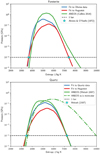 |
Fig. 11 Vapor curve for the different fits compared to the results from ANEOS. Top: case for forsterite. Bottom: case for quartz. We can see that our vapor curves fit the experimental entropy data very well and resemble the results from ANEOS with molecular gas. The critical pressure is generally lower for our models compared to the ANEOS model. For the forsterite vapor curve our model fits the experimental data better then the one from ANEOS (Collins & Melosh 2014). Experimental data for quartz is from Melosh (2007) and for forsterite is from Ahrens & O’Keefe (1972). |
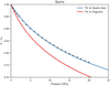 |
Fig. 12 Cold compression curve of quartz for the two different fits. We can see that the fit to the quartz material data fits very well with the experimental data, while the fit to the Hugoniot does not. The experimental data is from Kimizuka et al. (2007). |
Appendix A Equation of state (ρ∕ρ0 > 1)
A.1 Cold terms
The cold term of our EOS is based on the Varpoly EOS (Weppner et al. 2015), which polytrope exponent, bulk modulus and pressure is given by:
 (A.1)
(A.1)
 (A.2)
(A.2)
![Mathematical equation: \begin{align*} &P = \frac{B_0 e^{\frac{A_0}{A_{1}}}}{A_{1}}\left[\eta^{A_2}e_n\left(\frac{A_{1}+A_2}{A_{1}},\frac{A_0}{A_{1}}\eta^{-A_{1}}\right)-e_n\left(\frac{A_{1}+A_2}{A_{1}},\frac{A_0}{A_{1}}\right)\right],\\ &\eta = \frac{\rho}{\rho_0} \quad M=\frac{A_0}{A_{1}}\left(1-\eta^{-A_{1}}\right),\nonumber \end{align*}](/articles/aa/full_html/2020/03/aa35814-19/aa35814-19-eq48.png) (A.3)
(A.3)
where en is the exponential integral which can be written in terms of the incomplete gamma function.
 (A.4)
(A.4)
The cold internal energy term can be derived by integrating:
 (A.5)
(A.5)
In Zwillinger (2014) it is shown that the integral of the incomplete gamma function can be written as:
 (A.6)
(A.6)
Using variable substitution on dρ →dx we can find an expression for an energy function:
 (A.7)
(A.7)
![Mathematical equation: \[ \begin{array}{l} G = x^{n_2}\left[\Gamma(1-n_1,x)-\Gamma(1-n_1,x_0)\right]-\Gamma(1-n_1+n_2,x) \\ x = x_0 \eta^{-A_1} \quad x_0=\frac{A_0}{A_1}\\ n_1 = \frac{A_1+A_2}{A_1} \quad n_2=\frac{1}{A_1}. \end{array} \]](/articles/aa/full_html/2020/03/aa35814-19/aa35814-19-eq53.png)
A.2 Isothermal terms
The temperature dependent term, is given by the Dulong-petit limit, as we assume T ≫ θD within the Debye model:
 (A.8)
(A.8)
![Mathematical equation: \[ D(\theta_D/T)=\frac{3}{\left(\theta_D/T\right)^3}\int_0^{\theta_D/T} \frac{t^3}{\textrm{e}^t-1}\textrm{d}t\underset{T>>\theta_D}{\approx}1, \]](/articles/aa/full_html/2020/03/aa35814-19/aa35814-19-eq55.png)
 (A.9)
(A.9)
From the thermodynamic relationship
 (A.10)
We can get:
 (A.11)
Given the pressure and internal energy, the entropy and the rest of the thermodynamic potentials can be derived. Differentiation of the full pressure expression (cold + vibrational) while assuming constant temperature gives the following bulk modulus and polytrope exponent:
 (A.12)
 (A.13)
A.3 Adiabatic terms
Taking into account an adiabatic temperature gradient, gives the following bulk modulus and polytrope exponent9 :
 (A.14)
![Mathematical equation: \begin{equation*} B'_S=\frac{1}{1+\gamma \alpha T}\left[B'_T + \gamma \alpha T\left(2+\gamma-3q-\gamma \left(\frac{\partial \ln C_v}{\partial \ln T}\right)_V\right)\right]. \end{equation*}](/articles/aa/full_html/2020/03/aa35814-19/aa35814-19-eq62.png) (A.15)
(A.15)
A.4 Derivative of the Gruneisen parameter
The derivative of the Gruneisen parameter used in the adiabatic bulk modulus (Eq. (A.12)) is given below. The Gruneisen parameter is temperature independent, all the parameters given below are cold terms (T = 0).
 (A.16)
 (A.17)
![Mathematical equation: \[ \begin{array}{l} F = \frac{P}{B} N = \frac{B'}{2} - \frac{1}{6} \nonumber \\[5pt] F' = \frac{1 - FB'}{B} N' = \frac{B''}{2} \nonumber \\[5pt] D = 1 - \frac{2t}{3}F \tau = \frac{P}{3} t' \nonumber \\[5pt] D' = -\frac{2}{3} (Ft' + F't) \tau' = \frac{t'+Pt''}{3} \nonumber \\[5pt] T = \frac{t}{3}(1 - \frac{F}{3}) t' = -\delta_{t}\frac{t-t_{\infty}}{B} \nonumber \\[5pt] T' = \frac{t'}{3} + \frac{D'}{6} t'' = -\delta_{t}\frac{B'(t_{\infty}-t)+Bt'}{B^2} \nonumber\\[5pt] B'' = -\frac{A_{1}}{B}(B'-A_{2}). \end{array} \]](/articles/aa/full_html/2020/03/aa35814-19/aa35814-19-eq65.png)
Appendix B Equation of state (ρ∕ρ0 < 1)
B.1 Cold terms
The internalenergy is given by:
 (B.1)
(B.1)
The pressure is given by a Mie potential:
 (B.2)
(B.2)
 (B.3)
(B.3)
B.2 Thermal terms
The pressure and its derivatives retains the same form as in the compressed state. For the Gruneisen paramter an empirical fitting formula is used, which ensures that the Gruneisen parameter and its volume derivative are continuous at ρ0 and conform to the ideal gas law at zero density:
![Mathematical equation: \[ \gamma_k=1+\gamma_0-\gamma_{ideal}, \]](/articles/aa/full_html/2020/03/aa35814-19/aa35814-19-eq69.png)
 (B.4)
(B.4)
 (B.5)
(B.5)
where dexp is:
![Mathematical equation: \[ d_{\textrm{exp}}=q_0\gamma_0+c_{\textrm{exp}}\gamma_k. \]](/articles/aa/full_html/2020/03/aa35814-19/aa35814-19-eq72.png)
And cexp can be determined by the materials critical point temperature, or if not available set to around cexp = 0.6 ↔ 1.0.The heat capacity remains constant and the same as in the compressed state, which forces a lower Gruneisen parameter at the zero density limit to capture the correct ideal gas pressure.
![Mathematical equation: \[ \begin{array}{l} \gamma_{\textrm{ideal}}=\frac{1}{3}, \\ C_v=3Nk. \end{array} \]](/articles/aa/full_html/2020/03/aa35814-19/aa35814-19-eq73.png)
The total pressure P = PT0 + Pth can in this formulation become negative, this is by design to model the vapor phase change. For hydrodynamical simulations, when the material hits the vapor dome as presented in Sect. 4.4, the pressure in this region is replaced by the corresponding vapor pressure. If the vapor dome and the pressure have not been calculated, the total pressure can instead be set to zero and a minimum speed of sound enforced to avoid crashing the hydro simulation. The entropy and thermodynamical potentials in both the compressed and expanded state are given by:
![Mathematical equation: \[ \begin{array}{l} U=C_vT+\int \frac{P_{\textrm{cold}}}{\rho^2}\textrm{d}\rho, \\ S=C_v\ln T-C_v\int \frac{\gamma}{\rho}\textrm{d}\rho+S_{\textrm{ref}}, \\ F=U-TS=\int \frac{P_{\textrm{cold}}}{\rho^2}\textrm{d}\rho+C_v T\int \frac{\gamma}{\rho}\textrm{d}\rho - C_v T (\ln T - 1), \\ H=U-P/\rho, \\ G=F+P/\rho. \\ \end{array} \]](/articles/aa/full_html/2020/03/aa35814-19/aa35814-19-eq74.png)
Appendix C Vapor pressure within a hydrocode
In this section, we briefly explain how the vapor pressure is calculated for a material within a hydrocode. We first need to determine the boundary of the vapor curve, which is done prior to the start of the simulation. The boundary is given on a density/temperature (or internal energy) curve as seen in Fig. C.2. As a material decompresses it will eventually hit the vapor curve if the temperature is below the critical point. To get the pressure of the material within the coexistence region, we fit a function to the Arrhenius plot, seen in Fig. C.1. A suitable function for this curve is a simple exponential of the form Pvap = ea−b∕T. The fit parameters for forsteriteis a = 14.5 and b = 56 000 for P in MPa. Within the coexistence curve the bulk modulus is given by Bvap = γPvap (see Eq. (A.14)) which gives a sound speed of  ensuring that the material remains in a physical regime.
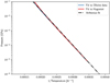 |
Fig. C.1 Vapor pressure vs. 1/T (Arrhenius plot). Used to calculate the vapor pressure within the vapor curve. Pressure on curve can be represented as P = ea−b∕T, fit parameters for forsterite is a = 14.5, b = 56 000 for P in MPa. |
 |
Fig. C.2 Generated vapor curve of temperature vs. density for forsterite. When the material enters a state that is within this curve the pressure is given by the vapor pressure as given by the Arrhenius curve (Fig. C.1). |
References
- Ahrens, T. J., & O’Keefe, J. D. 1972, Moon, 4, 214 [NASA ADS] [CrossRef] [Google Scholar]
- Al’Tshuler, L. V., Bakanova, A. A., Dudoladov, I. P., et al. 1981, J. Appl. Mech. Techn. Phys., 22, 145 [NASA ADS] [CrossRef] [Google Scholar]
- Anderson, O. L. 2007, GrÜneisen’s Parameter For Iron and Earth’s Core, eds. D. Gubbins & E. Herrero-Bervera (Dordrecht: Springer Netherlands), 366 [Google Scholar]
- Anderson, O. L., & Isaak, D. G. 2003, AGU Fall Meeting Abstracts [Google Scholar]
- Barr, A. C. 2016, J. Geophys. Res. Planets, 121, 1573 [NASA ADS] [CrossRef] [Google Scholar]
- Birch, F. 1947, Phys. Rev., 71, 809 [Google Scholar]
- Brown, J. M., Fritz, J. N., & Hixson, R. S. 2000, J. Appl. Phys., 88, 5496 [NASA ADS] [CrossRef] [Google Scholar]
- Brundage, A. L. 2013, Procedia Eng., 58, 461 [CrossRef] [Google Scholar]
- Burakovsky, L., & Preston, D. L. 2004, J. Phys. Chem. Solids, 65, 1581 [NASA ADS] [CrossRef] [Google Scholar]
- Calderon, E., Gauthier, M., Decremps, F., et al. 2007, J. Phys. Condens. Matter, 19, 436228 [CrossRef] [Google Scholar]
- Canup, R. M. 2012, Science, 338, 1052 [NASA ADS] [CrossRef] [Google Scholar]
- Canup, R. M., Barr, A. C., & Crawford, D. A. 2013, Icarus, 222, 200 [NASA ADS] [CrossRef] [Google Scholar]
- Citron, R. I., Genda, H., & Ida, S. 2015, Icarus, 252, 334 [NASA ADS] [CrossRef] [Google Scholar]
- Collins, G. S., & Melosh, H. J. 2014, Lunar Planet. Sci. Conf., 45, 2664 [NASA ADS] [Google Scholar]
- Connolly, J. A. D. 2016, J. Geophys. Res. Planets, 121, 1641 [NASA ADS] [CrossRef] [Google Scholar]
- Ćuk, M., & Stewart, S. T. 2012, Science, 338, 1047 [NASA ADS] [CrossRef] [Google Scholar]
- Debye, P. 1912, Ann. Phys., 344, 789 [CrossRef] [Google Scholar]
- Dewaele, A., Loubeyre, P., Occelli, F., et al. 2006, Phys. Rev. Lett., 97, 215504 [NASA ADS] [CrossRef] [Google Scholar]
- Dubrovinsky, L. S., Saxena, S. K., Dubrovinskaia, N. A., Rekhi, S., & Le Bihan T. 2000, Am. Mineral., 85, 386 [NASA ADS] [CrossRef] [Google Scholar]
- Dugdale, J. S., & MacDonald, D. K. 1953, Phys. Rev., 89, 832 [NASA ADS] [CrossRef] [Google Scholar]
- Dziewonski, A. M., & Anderson, D. L. 1981, Phys. Earth Planet. Inter., 25, 297 [NASA ADS] [CrossRef] [Google Scholar]
- Fischer, R. A. 2016, Melting of Fe Alloys and the Thermal Structure of the Core (New Jersey: John Wiley & Sons, Inc), 1 [Google Scholar]
- Gilvarry, J. J. 1956, Phys. Rev., 102, 308 [NASA ADS] [CrossRef] [Google Scholar]
- Grüneisen, E. 1912, Ann. Phys., 344, 257 [CrossRef] [Google Scholar]
- Irvine, R. D., & Stacey, F. D. 1975, Phys. Earth Planet. Inter., 11, 157 [NASA ADS] [CrossRef] [Google Scholar]
- Kimizuka, H., Ogata, S., Li, J., & Shibutani, Y. 2007, Phys. Rev. B, 75, 054109 [NASA ADS] [CrossRef] [Google Scholar]
- Krupnikov, K. K., Bakanova, A. A., Brazhnik, M. I., & Trunin, R. F. 1963, Sov. Phys. Dokl., 8, 205 [NASA ADS] [Google Scholar]
- Marinova, M. M., Aharonson, O., & Asphaug, E. 2008, Nature, 453, 1216 [NASA ADS] [CrossRef] [Google Scholar]
- Melosh, H. J. 2007, Meteorit. Planet. Sci., 42, 2079 [NASA ADS] [CrossRef] [Google Scholar]
- Mie, G. 1903, Ann. Phys., 316, 657 [CrossRef] [Google Scholar]
- Mosenfelder, J. L., Asimow, P. D., & Ahrens, T. J. 2007, J. Geophys. Res Solid Earth, 112, B06208 [NASA ADS] [CrossRef] [Google Scholar]
- Mosenfelder, J. L., Asimow, P. D., Frost, D. J., Rubie, D. C., & Ahrens, T. J. 2009, J. Geophys. Res Solid Earth, 114, B01203 [Google Scholar]
- Murphy, C. A., Jackson, J. M., & Sturhahn, W. 2013, J. Geophys. Res Solid Earth, 118, 1999 [NASA ADS] [CrossRef] [Google Scholar]
- Nagara, H., & Nakamura, T. 1985, Phys. Rev. B, 31, 1844 [NASA ADS] [CrossRef] [Google Scholar]
- Nakajima, M., & Stevenson, D. J. 2014, Icarus, 233, 259 [NASA ADS] [CrossRef] [Google Scholar]
- Panning, M., & Romanowicz, B. 2006, Geophys. J. Int., 167, 361 [NASA ADS] [CrossRef] [Google Scholar]
- Petrov, Y. 1994, High Press. Res., 11, 313 [NASA ADS] [CrossRef] [Google Scholar]
- Poirier, J.-P. 2000, Introduction to the Physics of the Earths Interior, 2nd edn. (Cambridge: (Cambridge University Press) [Google Scholar]
- Prescher, C., Dubrovinsky, L., Bykova, E., et al. 2015, Nat. Geosci., 8, 220 [NASA ADS] [CrossRef] [Google Scholar]
- Reinhardt, C., & Stadel, J. 2017, MNRAS, 467, 4252 [NASA ADS] [CrossRef] [Google Scholar]
- Root, S., Townsend, J. P., Davies, E., et al. 2018, Geophys. Res. Lett., 45, 3865 [NASA ADS] [CrossRef] [Google Scholar]
- Salpeter, E. E., &, Zapolsky, H. S. 1967, Phys. Rev., 158, 876 [NASA ADS] [CrossRef] [Google Scholar]
- Shanker, J., & Singh, B. P. 2005, Phys. B Condens. Matter, 370, 78 [NASA ADS] [CrossRef] [Google Scholar]
- Shanker, J., Singh, B. P., & Baghel, H. K. 2007, Phys. B Condens. Matter, 387, 409 [NASA ADS] [CrossRef] [Google Scholar]
- Slater, J. C. 1940, J. Soc. Chem. Ind., 59, 187 [Google Scholar]
- Stacey, F. D., & Davis, P. M. 2004, Phys. Earth Planet. Inter., 142, 137 [NASA ADS] [CrossRef] [Google Scholar]
- Stewart, S. T., Davies, E. J., Duncan, M. S., et al. 2019, arXiv e-prints, [arXiv:1910.04687] [Google Scholar]
- Stixrude, L., & Lithgow-Bertelloni, C. 2005, Geophys. J. Int., 162, 610 [NASA ADS] [CrossRef] [Google Scholar]
- Thompson, S. L., & Lauson, H. S. 1972, Improvements in the Chart D Radiation-Hydrodynamic Code. III: Revised Analytic Equations of State, Tech.rep. [Google Scholar]
- Tillotson, J. H. 1962, General Atomic Report GA-3216 [Google Scholar]
- Trunin, R. F., Simakov, G. V., Podurets, M. A., Moiseyev, B. N., & Popov, L. V. 1971, Izv. Akad. Nauk SSSR, Ser. Fizika Zemli, 1, 13 [Google Scholar]
- Vashchenko, V., & Zubarev, V. 1963, Sov. Phys. Solid State, 5, 653 [Google Scholar]
- Vinet, P., Ferrante, J., Rose, J. H., & Smith, J. R. 1987, J. Geophys. Res., 92, 9319 [NASA ADS] [CrossRef] [Google Scholar]
- Wackerle, J. 1962, J. Appl. Phys., 33, 922 [NASA ADS] [CrossRef] [Google Scholar]
- Weppner, S. P., McKelvey, J. P., Thielen, K. D., & Zielinski, A. K. 2015, MNRAS, 452, 1375 [NASA ADS] [CrossRef] [Google Scholar]
- Willis, B. T. M., & Pryor, A. W. 1975, Thermal Vibrations in Crystallography (London: Cambridge University Press) [Google Scholar]
- Wissing, R., & Hobbs, D. 2019, A&A, submitted (Paper II) [Google Scholar]
- Wu, Z. 2016, ArXiv e-prints, [arXiv:1611.00244] [Google Scholar]
- Xiao, B., & Stixrude, L. 2018, Proc. Natl. Acad. Sci., 115, 5371 [NASA ADS] [CrossRef] [Google Scholar]
- Zel’dovich, Y. B., & Raizer, Y. P. 1967, Physics of Shock Waves and High-temperature Hydrodynamic Phenomena (New York: Dover Publications) [Google Scholar]
- Zwillinger. 2014, in Table of Integrals, Series, and Products, 8th edn. (Boston: Academic Press), 623 [Google Scholar]
The pressure derivative of the bulk modulus is henceforth addressed as the polytrope exponent. It is however still denoted as B′.
Gruneisen parameter is independent of temperature, only accounts for acoustic modes and is a weighted average of modes ∑icviγi∕CV.
λ should go toward a finite value (Burakovsky & Preston 2004).
Maxwell construction was developed for the Van-der Waals EOS to replace the unstable sinusoidal behavior in the liquid–vapor phase transition with a constant vapor pressure. The vapor pressure is determined by a constant line that cuts the sinusoidal curve at three points in such a way that the work done between the three points is equal along the sinusoidal curve and the constant line
 .
.
Can be seen by calculating melting temperature from Lindeman’s law and comparing to the estimated Hugoniot temperatures.
However only the cold term in the free energy is modified during the solid–solid phase transition, which means that the phase change is independent of the temperature and only depends on the cold pressure.
This is a fit to olivine which is a mixture of the two endmembers forsterite Mg2 SiO4 and fayalite Fe2SiO4 which does have a slightly higher bulk modulus and density than pure forsterite.
The code used to make the analysis can be downloaded at https://github.com/robertwissing/EOS.
At constant pressure the bulk modulus does not go to zero, which means that the speed of sound remain physical during vapor transition.
All Tables
Quartz critical point parameters, estimate ranges are from Connolly (2016) and Melosh (2007).
Forsterite critical point parameters, estimate ranges are from Xiao & Stixrude (2018) and Connolly (2016) and experimental entropy estimate from Ahrens & O’Keefe (1972).
All Figures
|
Fig. 1 Isothermal expansion curve for α-quartz at different temperatures. The integral over the cold compression curve (blue) is equal to Evap. The minimum of the curve represents a point of instability. As we increase the temperature, we eventually reach the critical isotherm in which the minimum disappears. The critical point represents the point on the critical isotherm, in which the derivative goes to zero. Below the critical temperature the sinusoidal part of the curve is replaced by a constant vapor pressure using Maxwell construction. |
| In the text | |
|
Fig. 2 Compression curves of the different models and fits. The green line has been fit to the
ɛ-Fe data from Dewaele et al. (2006) using the Varpoly EOS ( |
| In the text | |
|
Fig. 3 Variation of the Gruneisen parameter with density for the different models and fits. The green line has been fit to experimental data from Anderson (2007) and Anderson & Isaak (2003) using our EOS with tmin = 1.94, δt = 3.89. The PREM curve was fit to ambient pressure values for ɛ-Fe given in Dubrovinsky et al. (2000) (γ0 = 1.78 q0 = 0.69). The Gruneisen parameter from the Tillotson EOS can be seen to have a completely different behavior than the rest. |
| In the text | |
|
Fig. 4 Poisson ratio curve of the compression fit and the PREM fit. The compression fit correlates excellent with the ɛ-Fe data from Murphy et al. (2013). To fit with the PREM data the PREM fit requires an unrealisticly high ambient Poisson ratio of ν0 = 0.4. This is mostlikely due to missing temperature dependent terms of the Poisson ratio for the PREM fit. |
| In the text | |
|
Fig. 5 Density model of Earth. Comparison between PREM and our fit. Material parameters for each layer is given in Table 1. |
| In the text | |
|
Fig. 6 Poisson ratio curve of the lower mantle. We can see that our PREM fit correlates well with the PREM data. The small discrepancy seen at 4400 kg m−3 is due to the transition from the previous planetary layer. |
| In the text | |
|
Fig. 7 Comparison of the different models to experimental Hugoniot data (Brown et al. 2000; Al’Tshuler et al. 1981; Krupnikov et al. 1963). The Hugoniot fit and the Tillotson fit correlate excellent with the experimental data. Surprisingly the PREM fit correlates well with the experimental data as well. |
| In the text | |
|
Fig. 8 Variation of the polytrope exponent with pressure. All of our EOS fits go to the predicted high pressure value. The Tillotson EOS however diverges around 1012 Pa and goes toward a higher asymptote |
| In the text | |
|
Fig. 9 Hugoniot curve for the different fits compared to the results from ANEOS (Stewart et al. 2019). The forsterite experimental data does not exhibit a sharp change as seen in the quartz data and here capturing the melt phase plays a larger role. Both ANEOS and our fit to the Hugoniot conform well with the data, while the fit to the quartz data over pressurizes within the range in which the material has melted (above 100 GPa). We also decided to plot the Tillotson EOS curve for olivine (Marinova et al. 2011), which diverges strongly from the experimental data after around 200 GPa. The experimental data is from Mosenfelder et al. (2007) and Root et al. (2018). |
| In the text | |
|
Fig. 10 Hugoniot curve for the different fits compared to the results from ANEOS (Collins & Melosh 2014). The experimental data show a sharp change at around
|
| In the text | |
|
Fig. 11 Vapor curve for the different fits compared to the results from ANEOS. Top: case for forsterite. Bottom: case for quartz. We can see that our vapor curves fit the experimental entropy data very well and resemble the results from ANEOS with molecular gas. The critical pressure is generally lower for our models compared to the ANEOS model. For the forsterite vapor curve our model fits the experimental data better then the one from ANEOS (Collins & Melosh 2014). Experimental data for quartz is from Melosh (2007) and for forsterite is from Ahrens & O’Keefe (1972). |
| In the text | |
|
Fig. 12 Cold compression curve of quartz for the two different fits. We can see that the fit to the quartz material data fits very well with the experimental data, while the fit to the Hugoniot does not. The experimental data is from Kimizuka et al. (2007). |
| In the text | |
|
Fig. C.1 Vapor pressure vs. 1/T (Arrhenius plot). Used to calculate the vapor pressure within the vapor curve. Pressure on curve can be represented as P = ea−b∕T, fit parameters for forsterite is a = 14.5, b = 56 000 for P in MPa. |
| In the text | |
|
Fig. C.2 Generated vapor curve of temperature vs. density for forsterite. When the material enters a state that is within this curve the pressure is given by the vapor pressure as given by the Arrhenius curve (Fig. C.1). |
| In the text | |
Current usage metrics show cumulative count of Article Views (full-text article views including HTML views, PDF and ePub downloads, according to the available data) and Abstracts Views on Vision4Press platform.
Data correspond to usage on the plateform after 2015. The current usage metrics is available 48-96 hours after online publication and is updated daily on week days.
Initial download of the metrics may take a while.