| Issue |
A&A
Volume 634, February 2020
|
|
|---|---|---|
| Article Number | A34 | |
| Number of page(s) | 15 | |
| Section | Stellar atmospheres | |
| DOI | https://doi.org/10.1051/0004-6361/201937055 | |
| Published online | 31 January 2020 | |
The Gaia-ESO Survey: a new approach to chemically characterising young open clusters
I. Stellar parameters, and iron-peak, α-, and proton-capture elements★,★★
1
Dipartimento di Fisica e Astronomia Galileo Galilei,
Vicolo Osservatorio 3,
35122
Padova,
Italy
e-mail: This email address is being protected from spambots. You need JavaScript enabled to view it.
2
INAF – Osservatorio Astronomico di Padova,
vicolo dell’Osservatorio 5,
35122
Padova,
Italy
3
Monash Centre for Astrophysics (MoCA), Monash University,
School of Physics and Astronomy,
Clayton,
VIC 3800,
Melbourne, Australia
4
INAF – Osservatorio Astrofisico di Arcetri,
Largo E. Fermi 5,
50125
Firenze, Italy
5
Instituto de Astrofísica e Ciências do Espaço, Universidade do Porto,
CAUP, Rua das Estrelas,
4150-762
Porto,
Portugal
6
Nicolaus Copernicus Astronomical Center, Polish Academy of Sciences,
ul. Bartycka 18,
00-716
Warsaw,
Poland
7
Institute of Theoretical Physics and Astronomy, Vilnius University,
Sauletekio av. 3,
10257
Vilnius, Lithuania
8
Departmento de Astrofísica, Centro de Astrobiología (INTA-CSIC), ESAC Campus, Camino Bajo del Castillo s/n,
28692
Villanueva de la Cañada,
Madrid, Spain
9
Instituto de Astrofísica de Andalucía-CSIC,
Apdo. 3004,
18080
Granada, Spain
10
Instituto de Física y Astronomía, Universidad de Valparaiso,
Gran Bretaña
1111,
Valparaíso
11
Núcleo Milenio de Formación Planetaria, NPF, Universidad de Valparaíso, Valparaíso, Chile
12
Lund Observatory, Department of Astronomy and Theoretical Physics,
Box 43,
221 00
Lund,
Sweden
13
INAF – Osservatorio di Astrofisica e Scienza dello Spazio di Bologna,
Via Gobetti 93/3,
40129
Bologna,
Italy
14
Institute of Astronomy, University of Cambridge,
Madingley Road,
Cambridge
CB3 0HA, UK
15
Observational Astrophysics, Department of Physics and Astronomy, Uppsala University,
Box 516,
75120
Uppsala, Sweden
16
INAF – Osservatorio Astronomico di Palermo,
Piazza del Parlamento 1,
90134
Palermo, Italy
17
European Southern Observatory,
Alonso de Cordova 3107 Vitacura,
Santiago de Chile,
Chile
18
Dipartimento di Fisica “Enrico Fermi”, Universita’ di Pisa,
Largo Pontecorvo 3,
56127
Pisa,
Italy
19
Núcleo de Astronomía, Facultad de Ingeniería, Universidad Diego Portales,
Av. Ejército 441,
Santiago, Chile
20
Astrophysics Group, Keele University,
Keele,
Staffordshire
ST5 5BG,
UK
21
McWilliams Center for Cosmology, Department of Physics, Carnegie Mellon University,
5000 Forbes Avenue,
Pittsburgh,
PA
15213, USA
22
School of Physics, University of New South Wales,
Sydney,
NSW
2052,
Australia
23
Centre of Excellence for All-Sky Astrophysics in Three Dimensions (ASTRO 3D),
Sydney,
Australia
Received:
5
November
2019
Accepted:
31
December
2019
Abstract
Context. Open clusters are recognised as excellent tracers of Galactic thin-disc properties. At variance with intermediate-age and old open clusters, for which a significant number of studies is now available, clusters younger than ≲150 Myr have been mostly overlooked in terms of their chemical composition until recently (with few exceptions). On the other hand, previous investigations seem to indicate an anomalous behaviour of young clusters, which includes (but is not limited to) slightly sub-solar iron (Fe) abundances and extreme, unexpectedly high barium (Ba) enhancements.
Aims. In a series of papers, we plan to expand our understanding of this topic and investigate whether these chemical peculiarities are instead related to abundance analysis techniques.
Methods. We present a new determination of the atmospheric parameters for 23 dwarf stars observed by the Gaia-ESO survey in five young open clusters (τ < 150 Myr) and one star-forming region (NGC 2264). We exploit a new method based on titanium (Ti) lines to derive the spectroscopic surface gravity, and most importantly, the microturbulence parameter. A combination of Ti and Fe lines is used to obtain effective temperatures. We also infer the abundances of Fe I, Fe II, Ti I, Ti II, Na I, Mg I, Al I, Si I, Ca I, Cr I, and Ni I.
Results. Our findings are in fair agreement with Gaia-ESO iDR5 results for effective temperatures and surface gravities, but suggest that for very young stars, the microturbulence parameter is over-estimated when Fe lines are employed. This affects the derived chemical composition and causes the metal content of very young clusters to be under-estimated.
Conclusions. Our clusters display a metallicity [Fe/H] between +0.04 ± 0.01 and +0.12 ± 0.02; they are not more metal poor than the Sun. Although based on a relatively small sample size, our explorative study suggests that we may not need to call for ad hoc explanations to reconcile the chemical composition of young open clusters with Galactic chemical evolution models.
Key words: stars: abundances / stars: fundamental parameters / stars: solar-type / open clusters and associations: general
Full Table 2 is only available at the CDS via anonymous ftp to cdsarc.u-strasbg.fr (130.79.128.5) or via http://cdsarc.u-strasbg.fr/viz-bin/cat/J/A+A/634/A34
Based on observations collected with the FLAMES instrument at VLT/UT2 telescope (Paranal Observatory, ESO, Chile), for the Gaia- ESO Large Public Spectroscopic Survey (188.B-3002, 193.B-0936).
Deceased.
© ESO 2020
1 Introduction
Open clusters (OCs) are among the most efficient objects with which the chemical properties and the evolution of the Galactic disc can be probed. These systems represent the concept of single stellar population well, that is, a group of coeval, (initially) chemically homogeneous stars. OCs cover a wide range in metallicity (between −0.3 and +0.4 dex), and most importantly, are almost ubiquitous in the Galactic disc. They therefore allow us to investigate a number of aspects, including stellar evolution and nucleosynthesis models, along with the radial and azimutal metallicity gradients (e.g. Friel 1995; Donati et al. 2015; Netopil et al. 2016; Jacobson et al. 2016; Reddy et al. 2016; Magrini et al. 2017).
In recent years, the number of studies on OCs and their characterisation has enormously increased through the data from several spectroscopic surveys (e.g. the APO Galactic Evolution Expreiment, APOGEE, Cunha et al. 2016, Donor et al. 2018, Carrera et al. 2019; and the Open Clusters Chemical Abundances from Spanish Observatories, OCCASO, Casamiquela et al. 2019 and references therein). However, while the number of studies on intermediate-age and old OCs (τ ≳ 600 Myr) is conspicuous, less attention has been payed to the chemical composition of young OCs (YOCs, ages younger than ~ 150 Myr) and star-forming regions (SFRs). The Gaia-ESO public spectroscopic Survey (Gilmore et al. 2012; Randich et al. 2013) places special emphasis on observations of OCs covering the age range from a few million to several billion years, analysed in a homogeneous way. It therefore offers the opportunity of deriving the metallicity and abundances of a significant number of young objects (Spina et al. 2014a,b). The study of such systems is indeed very important to shed light on different topics, such as the metallicity distribution in the solar neighbourhood, the present-day metallicity distribution in the Galactic disc (Spina et al. 2017), the connection between the occurrence of giant planets and metallicity of the host stars (e.g. Santos et al. 2003), and the behaviour of heavy-element (slow n-capture process) abundances (see e.g. D’Orazi et al. 2017a and references therein).
Somewhat at odds with what is expected from the Galactic chemical evolution models, several authors found that no YOCs or SFRs with super-solar metallicities exist (James et al. 2006; Santos et al. 2008; D’Orazi et al. 2011; Biazzo et al. 2011a,b; Spina et al. 2014a,b, 2017; Origlia et al. 2019). All the young populations in the solar neighbourhood seem to be slightly metal poor with respect to the Sun. The presence of these systems might be explained with a complex combination of star formation, gas inflows and outflows, radial migration (Minchev et al. 2013), or a different composition of the parental molecular cloud (Spina et al. 2017).
It is well established that the frequency of giant planets is higher around metal-rich stars, and this is predicted by planet formation models (core accretion; Pollack et al. 1996; and the recent tidal downsizing models; Nayakshin 2017). The lack of metal-rich YOCs and SFRs could influence this relation, and the question arises whether it is less probable to find giant planets in these systems. There is growing observational evidence that in some cases, the planetary companion might be more metal rich than the host star (Vigan et al. 2016, Samland et al. 2017), as predicted by the core accretion paradigm. However, the uncertainty on the metallicity of the young stars hosting planets, with typical uncertainties of ~0.2 dex (e.g. James et al. 2006), prevents us from placing strong constraints on this aspect. This topic clearly deserves deeper investigation.
There are reasons to think that the sub-solar metallicity of young stars is not intrinsic, but related to analytical problems. Young stars have active chromospheres that may affect line formation and thus the derived stellar parameters and abundances. They also have intense magnetic fields (Folsom et al. 2016) that might be related to different phenomena and mechanisms. For instance, James et al. (2006) and Santos et al. (2008) reported extremely high values of microturbulence parameters (ξ) (up to ~ 2.5 km s−1), along with a substantial star-to-star variation (that is apparently unrelated to the other stellar parameters: two stars in IC 4665 analysed by Gaia-ESO have a difference in temperature of +90 dex according to the iDR5 results and a difference in log g of +0.01 dex, but a difference in ξ of +0.70 kms−1). A similar behaviour has also been reported (Viana Almeida et al. 2009), who analysed stars in 11 associations containing young stars, and found ξ values up to ~ 2.6 km s−1. Moreover, the authors reported a weak trend of ξ with the effective temperature (Teff), with higher values at lower Teff.
Recently, Reddy & Lambert (2017) have investigated a possible correlation between Fe I abundances and the line formation optical depth. According to their results, the Fe I lines that form in the upper layers of the photosphere in young active stars provide larger abundances than those forming in the lower layers, probably because of the active chromosphere. This trend may also affect the value of ξ when it is derived by removing the slope between individual Fe I line abundances and their reduced equivalent widths (REWs). ξ is a free parameter introduced to account for the difference between the observed equivalent widths (EWs) of moderate to strong lines and those predicted by models based on thermal and damping broadening alone. Weaker lines are almost independentof this parameter; it is therefore calculated by forcing weak and strong lines to be in agreement. If strong lines (typically forming in the upper photospheric layers) yield anomalously larger abundances than weaker lines, ξ needs to be increase in order to remove the slope. Galarza et al. (2019) recently reported on the effects of stellar activity on the stellar parameters, but their analysis involved a star that is much older (τ ~400–600 Myr) than those in our sample.
Another important aspect is the behaviour of the s-process elements. D’Orazi et al. (2009) found that the [Ba/Fe] ratio is positively correlated with OC ages. The standard analysis of the Ba II 5853 Å and 6496 Å lines gave values up to +0.60 dex in clusters younger than 50 Myr, but solar values in older clusters (age ≳ 1–2 Gyr). The increasing trend as a function of the age has been confirmed by other authors (Maiorca et al. 2011; Jacobson & Friel 2013; Mishenina et al. 2015; Reddy & Lambert 2017; Magrini et al. 2018; Delgado Mena et al. 2019), and it has been interpreted by Maiorca et al. (2012) as due to the recent production by nucleosynthesis in asymptotic giant branch (AGB) starsof low mass. This can explain mild enhancements (up to 0.1–0.2 dex), but not the much higher values measured invery young clusters, however. Of the different explanations, the sensitivity of the Ba II 5853 Å line to the ξ parameter value seems to be the most promising (Reddy & Lambert 2015). The Ba II 5853 Å forms in the upper layers of the photosphere, where the effects of the active chromosphere are stronger. All these pieces of evidence support our hypothesis that the standard chemical analysis in very young stars (τ < 150 Myr) might lead to misinterpreted results. We will investigate the behaviour of s-process elements and their time evolution in a companion paper (Baratella et al., in prep.).
In this first paper of a series focused on the chemical characterisation of very young stars, we propose a new approach to perform the chemical analysis of these young objects. We analyse Gaia-ESO fifth internal data release (iDR5) spectra of 23 stars observed in five YOCs plus one SFR by the Gaia-ESO Survey. The dataset is described in Sect. 2. In Sect. 3 we derive the input values of the atmospheric parameters from photometry. We determine the stellar parameters by employing a new method (Sect. 4) that is almost entirely based on the use of titanium lines. We also derive abundances for different α-, proton-capture, and iron-peak elements: Fe I, Fe II, Ti I, Ti II, Na I, Mg I, Al I, Si I, Ca I, Cr I, and Ni I. In Sects. 5 and 6 we present our results and discuss the scientific implications.
2 Dataset
We analyse high-resolution (R ~ 47 000) spectra of 23 solar-type dwarf stars (with spectral type from F9-K1) in five YOCs and one SFR, observed in the Gaia-ESO Survey. The selected targets are IC 2391, IC 2602, IC 4665, NGC 2264, NGC 2516, and NGC 2547, all with ages younger than 150 Myr. We have chosen these clusters because no observational studies have been carried out in the framework of heavy-element abundances, with the exception of IC 2391 and IC 2602, which we used as calibrators of our abundance scale. Some information on these objects is reported in Table 1.
The spectra of the target stars were acquired with the high-resolution Fiber Large Array Mulit-Element Spectrograph and the Ultraviolet and Visual Echelle Spectrograph (FLAMES-UVES; Pasquini et al. 2002) and have been reduced by the Gaia-ESO consortium in a homogeneous way. The data reduction of UVES spectra was carried out using the FLAMES-UVES ESO public pipeline (Modigliani et al. 2004; Sacco et al. 2014).
Different Working Groups (WGs) contribute to the spectrum analysis: for the stars considered here, the analysis was performed by WG11 and WG12. The details of the procedures are described in Smiljanic et al. (2014) and Lanzafame et al. (2015). The recommended parameters produced by this analysis are reported in the iDR5 catalogue and are used as comparison for the results we obtained with our new approach.
The UVES observations were performed with the 580 nm setup for F-, G-, and K-type stars, with the spectra covering the 4800–6800 Å wavelength range. In particular, this spectral range contains the 6708 Å line of 7Li, which is an important diagnostic of stellar age. We did not consider the GIRAFFE spectra because their spectral range is limited and they have a lower resolution. Of all the available spectra, we selected only stars with rotational velocities v sin i < 20 km s−1 to avoid significant or heavy line blending, with signal-to-noise ratios (S/N) higher than 50 and effective temperatures Teff ≳ 5200 K to avoid over-ionisation and/or over-excitation effects (Schuler et al. 2010). All selected stars are confirmed members of corresponding clusters through radial velocities (RVs) and the strength of the 7Li absorption line at 6708 Å, according to the Gaia-ESO iDR5 measurements.
Basic information of the SFR and YOCs investigated in this work.
3 Input estimates of the atmospheric parameters
Teff estimates were obtained using photometry from the Two Micron All-Sky Survey (2MASS; Cutri et al. 2003) with the calibrated relation by Casagrande et al. (2010), valid for (J− K) de-reddened colours in the range  mag. We used this photometry because it provides homogeneous data for the stars in this study.
We used the classical equation for the surface gravity (log g),
 (1)
(1)
where Teff,⊙ = 5771 K, log g⊙ = 4.44 dex, and MBC,⊙ = 4.74. Teff is the T(J−K) estimate and MK is the absolute magnitude in K band, calculated with the distance estimates reported in Table 1. BCK is the bolometric correction in K band, calculated as in Masana et al. (2006). The values of m⋆ were estimated using the Padova suite of isochrones (Marigo et al. 2017). From these, we infer the mass to be equal to 1 M⊙ for the five YOCs, while for the stars in the SFR, we infer m⋆ = 2–3 M⊙.
The ξ values were derived using the Gaia-ESO relation (Worley et al., in prep.), calibrated for warm main-sequence stars:
![Mathematical equation: \begin{equation*} \begin{split} \xi \,{=}\,&1.10 + 6.04\,10^{-4}\cdot(T_{\textrm{eff}}-5787) + 1.45\,10^{-7}\cdot(T_{\textrm{eff}}-5787)^2\\ &-3.33\,10^{-1}\cdot(\log g-4.14) + 9.77\,10^{-2}\cdot(\log g-4.14)^2\\ &+6.94\,10^{-2}\!\cdot(\textrm{[Fe/H]}+0.33) + 3.12\,10^{-2}\!\cdot(\textrm{[Fe/H]}+0.33)^2, \end{split} \end{equation*}](/articles/aa/full_html/2020/02/aa37055-19/aa37055-19-eq3.png) (2)
(2)
which is valid for stars with Teff ≥ 5200 K and log g ≥ 3.5 dex. In all the calibrated relations used to derive Teff, the bolometric correction, and ξ, the input metallicity was assumed to be solar, which was later confirmed by the chemical abundances analysis. The input values of the atmospheric parameters for all the stars are reported in Tables A.1 (i.e. Teff,phot) and A.2 (i.e. log gphot and ξphot).
4 New approach in elemental abundance analysis
To derive spectroscopic atmospheric parameters and element abundances of our target stars, we used thelocal thermodynamic equilibrium (LTE) line analysis and synthetic spectrum code MOOG1 (version 2017, Sneden 1973; Sobeck et al. 2011). Abundances of Fe I, Fe II, Ti I, Ti II, Na I, Mg I, Al I, Si I, Ca I, Cr I, and Ni I were estimated using the EW method with the abfind driver.
We used 1D model atmospheres that we linearly interpolated from MARCS grid (Gustafsson et al. 2008), in the assumption that LTE and plane-parallel geometry is valid for dwarf stars. We chose these atmosphere models to be consistent with the analysis of the UVES spectra performed by the Gaia-ESO consortium. The lines we used were taken from D’Orazi et al. (2017b), originally selected from the line list optimised for solar-type stars from Meléndez et al. (2014). We cross-matched our original line list with the official Gaia-ESO line list (Heiter et al. 2019) to adopt the same atomic parameters, in particular the value for the oscillator strength (log gf). The complete line list can be found in Table 2. We used the Barklem prescriptions for damping values (see Barklem et al. 2000 and references therein).
The EWs for all the lines were measured using the software ARESv2 (Sousa et al. 2015)2. We discarded all the lines with uncertainties larger than 10% and those lines with EWs >120 mÅ because stronger lines cannot be fitted with a Gaussian profile. In some cases, especially for stars with relatively high rotational velocities, we added lines by measuring their EWs by hand using the task splot in IRAF.
Atomic line data.
Atmospheric parameters and chemical composition of Gaia benchmarks stars.
4.1 Standard analysis: iron lines
First, we applied the standard analysis, which only uses neutral and ionised Fe lines to derive Teff from the excitational equilibrium, log g by imposing the ionisation equilibrium, and ξ by zeroing the trend with the REWs. We analysed the Sun and the Gaia FGK benchmark stars α Cen A, τ Cet, β Hyi, and 18 Sco, whose UVES spectra were taken from Blanco-Cuaresma et al. (2014). The atmospheric parameters for the Gaia benchmark stars are listed in Table 3. We selected only these four benchmark stars because their atmospheric parameters are similar to those of the stars in our sample. In addition, we analysed one star of the first calibrator cluster IC 2391 (age ~ 50 Myr), 08365498−5308342. We obtain Teff = 5350 ± 100 K, log g = 4.51 ± 0.15 dex, ξ = +1.75 ± 0.10 km s−1, and [Fe/H] = − 0.07. These values are similar to the iDR5 results, which are Teff = 5381 ± 55 K, log g = 4.49 ± 0.06 dex, ξ = +1.77 ± 0.01 km s−1, and [Fe/H] = − 0.09.
We investigated the nature of this quite high ξ value in more detail by synthesising all the Fe lines with the code MOOG. Figure 1 shows that the synthetic profile with the anomalous value of ξ (in red) does not reproduce the observed line profile (in black) in the weak or strong lines, which confirms our suspicion that the ξ value is too high. This behaviour is confirmed in 90% of the Fe lines of the line list. Instead, the synthetic profile with the atmospheric parameters, in particular ξ = 0.85 ± 0.10 km s−1, that we derived with the new method described in Sect. 4.2 (blue line) reproduces the observed profile better.
4.2 Titanium and iron lines
We derived the atmospheric parameters using the second element with the largest number of spectral lines measurable in our stellar types, both of the neutral and the ionised species: titanium. On average, Ti lines form deeper in the photosphere than the Fe lines, at log τ5000 ~−1, where log τ5000 is the optical depth expressed in the logarithmic scale and calculated at the 5000 Å reference wavelength. We therefore expect little influence from the chromosphere, that is, a lack of trends between abundances and line formation depth. Moreover, we have very precise laboratory measurements of the log gf values from Lawler et al. (2013) for the Ti lines. Recently, Tsantaki et al. (2019) have argued that especially for cool dwarf stars, the atmospheric parameter values derived with Ti lines are more reliable than those derived with Fe lines. However, the authors used Ti lines only to impose the ionisation balance, in order to infer surface gravity estimates. Here we expand upon this approach.
The excitation potential (E.P.) range covered by the Ti lines used here is unfortunately too narrow to obtain a reliable estimate of Teff (from 0 to 2.0 eV, while for Fe the rangeis 0–5.0 eV). All Teff values we obtained with Ti lines alone are higher than the photometric estimates (200–300 K higher), and the uncertainties are of about 200 K. Moreover, in some stars, especially those with higher rotational velocities, the number of measurable Ti lines is very low, in some cases there are even fewer than ten lines, as we show in Fig. 2.
To obtain more lines and a wider coverage of the E.P. range, we derived Teff values using Fe I and Ti I lines simultaneously. Tables 3 and A.1 show that the agreement between the three different estimates of Teff is very good. Instead, for the other parameters we used Ti lines alone for the reasons presented above.
In summary, our new approach consists of the following three steps:
-
deriving Teff by zeroing the trend between E.P. and abundances of Ti I and Fe I lines simultaneously (in particular, the slope of the trend is lower than the uncertainty on the slope, and the trend is not statistically meaningful);
deriving log g by imposing the ionisation equilibrium for Ti lines alone, that is, the difference between Ti I and Ti II is of the order of the quadratic sum of the uncertainties calculated by MOOG divided by the square root of the number of lines of the two species;
deriving ξ by zeroing the trend between the REW of Ti I lines alone and the abundances (as for the temperature, the slope of the trend is expected to be lower than the uncertainty on the slope).
When the star had fewer than ten measurable Ti I lines, we kept the ξ value fixed to the photometric estimate (7 of 23 stars). We considered 2 stars with discrepant ξ values: 17452508+ 0551388 (IC 4665, age 40 Myr) and 08110139−04900089 (NGC 2547, age 50 Myr). We re-derived the atmopsheric parameters keeping the ξ value fixed to the photometric guess. We find that for 17452508+0551388 the new parameters are equal to Teff = 5321 ± 150 K, log g = 4.35 ± 0.10 dex, and ξ = 0.75 ± 0.04 km s−1, while for 08110139−04900089, we find Teff = 5325 ± 100 K, log g = 4.47 ± 0.10 dex, and ξ = 0.80 ± 0.04 km s−1. The difference between the newly derived Teff and those we derived with our method is lower than 50 K and lower than the typical error (75–100 K) we obtain for the Teff parameter. We therefore conclude that the two Teff measurements are consistent and that the effect of these differences on the final metallicity values is weak. For the Sun, we measure 11 Ti II lines, and for our sample stars we measure from 4 to 8 lines, depending on the quality of the spectra. Figure 3 shows an example of the trends with the final parameters for star 08365498−5308342. In the y-axis of the top panel, the difference between individual lines and the mean values per atomic species is reported and was calculated as  . The trend between Fe I line abundances and REWs clearly suggests that the ξ value needs to be further increased.
All the final abundances were calculated differentially with respect to the Sun. The final model atmospheres and abundances are reported in Table A.2. We also calculated the abundances for other different α- and proton-capture and iron-peak elements, in particular, Na I, Mg I, Al I, Si I, Ca I, Cr I, and Ni I. The respective abundance ratios [X/Fe] were calculated as [X/Fe] = [X/H]⋆−[Fe/H]⋆ (in particular, [Ti/Fe]II = [Ti/H]II−[Fe/H]II). The final abundance ratios are reported in Table A.3.
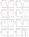 |
Fig. 1 Examples of the synthesis of several Fe I lines of star 08365498−5308342 (v sin i = 9.88 km s−1, as the recommended value given in the iDR5) for which the observed profile is not fitted when we adopt the ξ value obtained from the Fe lines (ξ = 1.75 km s−1; red line) and with the values derived with the new method (ξ = 0.85 km s−1; blue line). |
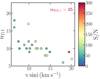 |
Fig. 2 Number of Ti I lines measured for each star as a function of S/N, colour-coded according to v sin i <20 km s−1. Stars with similar S/N but higher rotational velocities have fewer measurable lines. The number of Ti I lines measured in the Sun is reported in the top right corner. |
4.3 Solar abundance scale and the Gaia benchmark stars
We applied our new method to the Gaia benchmark stars to determine its validity, and to the solar spectrum to derive our solar abundance scale. In Table 3 we report the values of the atmospheric parameters and abundances of the Gaia benchmark stars. The results we obtain with our new method are in excellent agreement with the results by Jofré et al. (2015, 2018) and with Gaia-ESO, in particular for ξ (rows highlighted in yellow). We obtain very similar results, which confirms our hypothesis that the standard analysis produces good results for older stars (≳ 600 Myr).
In Table 4 we report the solar abundance scale, obtained with the atmospheric values reported in Table 3. The mean value between Fe I and Fe II for the final Fe abundance is reported, also for Ti. The uncertainties are the quadratic sum of the σ1 and σ2 contributions (calculated as the scatter measured by MOOG divided by the square root of the number of lines and as the sensitivity of the abundances to uncertainties in the atmospheric parameters, respectively). Our solar abundances generally agree well with the results by Asplund et al. (2009), with the meteoritic results by Lodders et al. (2009), and also with the results of Gaia-ESO iDR5. Based on the study of Bergemann (2011) on the NLTE effects on Ti, we expect that NLTE corrections for our lines that form at log (τ5000) ~−1 and at solar metallicities are negligible.
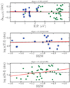 |
Fig. 3 Example of applying the new method for star 08365498−5308342 (IC 2391, age 50 Myr). The green dots represent the Fe I lines, and the blue squares represent the Ti I lines; the red lines in both panels are the linear regression, and individual slope and uncertainties are reported for each panel. See text for further details. |
Solar abundances derived here and in Asplund et al. (2009, A09), and meteoritic abundances from Lodders et al. (2009, L09).
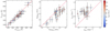 |
Fig. 4 Comparison between the photometric and spectroscopic estimates of the atmospheric parameters. The red line represents the 1:1 relation. The points are colour-coded according to ages. The red points refer to NGC 2516, and the blue points to the younger clusters. |
4.4 Uncertainty estimates
The uncertainties of the atmospheric parameters reported in Tables A.1 and A.2 were estimated as follows.  was calculated by varying the temperature until the slope E.P. versus abundance was larger than its uncertainty and the trend became statistically meaningful. σlog g was estimated by varying log g until Δ(Ti II−Ti I) was larger than the quadratic sum of the uncertainties. Finally, σξ was calculated by varying ξ until the slope of the trend was larger than the uncertainty on the slope and the trend became statistically meaningful. We individually evaluated the uncertainties for each star; in general, they are about 75–100 K, 0.10 dex, and 0.10–0.15 km s−1 for Teff, log g, and ξ, respectively.
The uncertainties on the abundances, σ1 and σ2 reported in Table A.2, take the internal uncertainties and the contribution of the atmospheric parameters into account, respectively. The first source of uncertainty, σ1, can be represented by the standard deviation from the mean abundance considering all the lines divided by the square root of the number of lines. The σ2 values instead represent the sensitivity of [X/H] to the uncertainties in the atmospheric parameters, and this sensitivity is calculated as
![Mathematical equation: \begin{equation*} \sigma_2\,{=}\,\sqrt{\left( \sigma_{T_{\textrm{eff}}} \frac{\partial {\textrm{[X/H]}}}{\partial T_{\textrm{eff}}}\right) ^2 + \left( \sigma_{{\log\,g}} \frac{\partial {\textrm{[X/H]}}}{\partial {\log g}}\right) ^2 +\left( \sigma_{\xi} \frac{\partial {\textrm{[X/H]}}}{\partial {\xi}} \right) ^2}. \end{equation*}](/articles/aa/full_html/2020/02/aa37055-19/aa37055-19-eq6.png)
As reported in Table A.3, for the uncertainties of the abundance ratios [X/Fe], the σ1 values were calculated by quadratically adding the σ1 value of [Fe/H] and that of [X/H]. The σ2 values were instead calculated in the same way as for [X/H].
5 Results and discussion
5.1 Stellar atmospheric parameters
The atmospheric parameters we inferred with our method agree well with the photometric estimates (Fig. 4, where the data are colour-coded according to age). The temperatures agree very well, with a mean difference of −37 ± 49 K. We note a general offset of the log g values, with a difference of −0.11 ± 0.09 dex. However, we also note that the ionisation equilibrium is valid for both Ti and Fe (Table A.2). For the ξ values, we find instead that the spectroscopic estimates are slightly larger than the photometric ones, but still comparable, with a difference of 0.15 ± 0.10 km s−1. We excludedall stars from the comparison plots whose ξ value was fixed to the photometric estimate. However, this offset between spectroscopic and photometric determinations of ξ is known in the literature and has also been observed in old stars. We note that using the values derived by Gaia-ESO (~ 2.0 km s−1), the difference with the photometric estimates is even larger.
We compared our results of the atmospheric parameters and the Fe and Ti abundances with those given in the iDR5 catalogue. The comparison plots are shown in Fig. 5 (as in Fig. 4, the data are colour-coded by age): our measurements of Teff and log g are in fair agreement with Gaia-ESO. For Teff we obtain mean differences between our values and Gaia-ESO results of −66 ± 122 K. Instead, for log g we found Δlog g = − 0.07 ± 0.11 dex. We conclude that our results are reliable and agree with those of Gaia-ESO. However, the largest differences are seen for the ξ parameter. Our results are lower than those of iDR5. We find a mean difference of −0.46 ± 0.36 km s−1. A small mean difference like this can be explained by the fact that for the stars in NGC 2516 (τ ~ 130 Myr), we obtain values of ξ that agree with iDR5.
The third panel in the top row in Fig. 5 shows a net separation between younger OCs and older OCs (in this case, only NGC 2516, represented by the red points). The most dramatic effect of over-estimating the ξ value is seen in the youngest clusters. We calculated the mean differences for the clusters with ages younger than 100 Myr and for NGC 2516 with ages older than 100 Myr. While the oldest cluster has a mean difference of −0.23 ± 0.13 km s−1, meaning that our results are comparable to the iDR5 results, for the youngest clusters we have a mean difference of −0.85 ± 0.27 km s−1, which is significant at the 3σ level. These results confirm our hypothesis that the standard analysis might produce over-estimated values of the ξ parameter for young stars, which leads to an under-estimation of the element abundances, as is shown in the bottom panels of Fig. 5.
It is noteworthy that for the NGC 2516 stars we derive a slightly higher metallicity than was published by Gaia-ESO, although the ξ values are quite similar. In particular, even if the difference in ξ is smaller than the difference with the younger stars, the range covered by the difference in [Fe/H] is the same as for the younger stars. This can be explained as the result of small differences in the other photospheric parameters (e.g. 100 K in temperature produces 0.07 dex in metallicity), to the use of different criteria in zeroing the trends in order to derive the photospheric parameters, to the use of different method, such as the spectral synthesis, and to differences in the EW measurements.
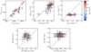 |
Fig. 5 Comparison between the values of Teff,spec, log gspec, ξspec, and [X/H] derived here with the values from Gaia-ESO iDR5. The red line represents the 1:1 relation. We exclude stars from the plot whose ξ value is fixed to the photometric estimates. See text for further details. |
Mean abundances and abundance ratios of each cluster.
5.2 Element abundances
Final parameters and abundance ratios are reported in Tables A.2 and A.3. The mean values for each cluster are reported in Table 5, where the uncertainties represent the uncertainty on the mean. In some cases it was not possible to derive the abundances of some element, such as Al I, because the lines were too weak to be measured or because of blending with nearby lines.
To evaluate the validity of our method, we determined the correlation between the derived abundances with Teff, as in Fig. 6 for Fe and Ti and Fig. 7 for the different [X/H] ratios. We also determined the trends between [X/H] and log g (Fig. 8). In these figures, the data are colour-coded according to the age, as for the previous plots. The α- and proton-capture and the iron-peak elements overall show solar abundances, as expected for these types of objects. We do not find any statistically meaningful trend, therefore our results are expected to be reliable.
Originally, our sample included a few stars with Teff ≲ 5200 K. For these stars we find discrepancies (differences larger than 0.8 dex) between abundances derived from Fe I and Fe II, as well as Ti I and Ti II. These can be explained with the so-called overionisation effect. It has been confirmed by different authors that stars with Teff≲ 5200 K and young ages (τ ≲ 100 Myr) show systematically larger Fe II abundances with respect to Fe I in clusters and in field stars (King et al. 2000; Chen et al. 2008; Schuler et al. 2010; Bensby et al. 2014). These differences are stronger as Teff decreases and dramatically affect the derived atmospheric parameters values, in particular log g. This is also valid for the Ti lines (see Fig. 4 in D’Orazi & Randich 2009). According to the results reported by D’Orazi & Randich (2009), the over-ionisation effect reaches values up to 0.6 dex for stars with Teff lower than 5000 K, which decrease with increasing Teff. Over-ionisation and/or over-excitation effects drove our choice to restrict the analysis to star with Teff≳ 5200 K.
We compared our final mean results with literature values. For IC 2391, IC 2602, IC 4665, and NGC 2516, our measurements in general agree fairly well with different studies (De Silva et al. 2013, D’Orazi & Randich 2009, Shen et al. 2005, and Terndrup et al. 2002, respectively). For NGC 2264, King et al. (2000) derived abundances for three stars and obtained a mean metallicity of −0.15 ± 0.09. King et al. (2000) studied two stars with Teff < 5000 K and one star that was similar to the Sun. The authors derived Teff and ξ with the standard spectroscopic analysis, but they fixed log g to the value estimated based on the isochrones. Their Table 1 lists ξ values of ~2.0 kms−1, which causes the Fe abundances to become sub-solar.
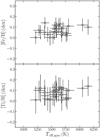 |
Fig. 6 [Fe/H] (top panel) and [Ti/H] (bottom panel) as a function of Teffderived using Fe and Ti lines simultaneously. For Fe, the Pearson correlation coefficient is r = 0.35, with p = 0.10, which is not significant at p < 0.05. For Ti, the Pearson correlation coefficient is r = 0.32, with p = 0.14, which is not significant at p < 0.05. |
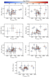 |
Fig. 7 [X/H] as function of Teff, derived with the new method and colour-coded according to age. |
5.3 Effect of stellar activity
To analyse the effect of stellar activity on Fe lines, we studied the dependence of the Fe line EWs on optical depth log τ5000, taken from Gurtovenko & Sheminova (2015). In Fig. 9, we calculate the difference of the EWs of the Fe and Ti lines between a solar analogue (star 10442256−6415301 belonging to IC2602, with an age of 30 Myr) and the Sun. The solar analogue has Teff = 5775 ± 75 K and log g = 4.49 ± 0.10 dex, and we assumed that the metallicity is the same as the Sun. Lines forming in the upper layers of the atmosphere (log τ5000 < −2.5) in the young star have larger EWs than those in the Sun, with differences up to 5–10 mÅ. The linear trend for the Fe lines has a Pearson correlation coefficient r = −0.85 and is significant at p < 0.01. Lines forming in the external layers are much stronger in the young star than in the Sun; this means that this effect can influence the derivation of the ξ parameter when it is derived based on the Fe lines.
We also analysed the dependence of the ξ parameter on the chromospheric activity index  . Because we cannot directly calculate
  from our spectra (because the spectral coverage does not include the Ca II H and K lines), we used theconversion relation found in Mamajek & Hillenbrand (2008), which takes the log (LX∕Lbol) activity index into account. We find in the literature values for 14 of the 23 stars we analysed. Figure 10 shows that while our measurement does not display a significant trend with activity, the ξ values measured by Gaia-ESO instead increase at increasing
  , that is, at an increasing level of activity. In this figure, we also report the values for the Gaia benchmark stars we analysed. The benchmarks are quiet stars, with
  , and we obtain the same value as Jofré et al. (2015) with the new approach, as reported in Table 3. We also note that the ξ value we obtain for β Hyi is slightly higher than the values obtained for the other benchmark stars, which is mainly due to the slightly advanced evolutionary stage.
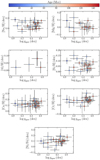 |
Fig. 8 [X/H] as function of log g, derived using only Ti lines and colour-coded according to age. |
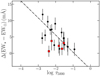 |
Fig. 9 Difference between the EWs of the Fe (black dots) and Ti (red dots) lines measured in the solar-analogue star 10442256−6415301 (30 Myr)and the Sun as a function of the optical depth of line formation log τ5000. The dot-dashed line is the trend for Fe lines. |
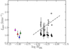 |
Fig. 10 Activity index |

6 Concluding remarks
We proposed a new approach to deriving the stellar atmospheric parameters. We analysed a sample of 23 dwarf stars observed in five Galactic YOCs and one SFR that are included in the Gaia-ESO survey.
In particular, for a young cluster star an EW analysis that only uses Fe I lines returns a value for the ξ parameter that is too high, as shown by the model lines, which are too strong compared to the observed lines. This indicates that the derived Fe line abundances depend on the optical depth of line formation, as suggested by Reddy & Lambert (2017). We also confirm thatthis effect is weak in old stars, as we showed for the Gaia benchmark stars, for which we obtain the same results as Jofré et al. (2015, 2018) and Gaia-ESO.
Our method consists of a combination of Fe and Ti lines to derive Teff by zeroing the trend between the individual line abundances and the E.P. For log g and the ξ parameter, we only use Ti lines to avoid possible complications due to the use of Fe lines, because the Fe lines form in a wider range of optical depth and the strongest lines can be affected by the hot active chromosphere. The comparison with Gaia-ESO iDR5 results showed that while for Teff and log g we obtain comparable measurements, a most dramatic effect is seen for ξ. Overall, we note an overestimation of this parameter, with the largest differences seen for clusters younger than 100 Myr.
We plot the metallicity distribution as a function of the open cluster age in Fig. 11, where the empty circles represent the clusters in Netopil et al. (2016) for which high-quality determination of metallicity are available (Heiter et al. 2014) and with 7.5 < RGal < 9 kpc. The coloured stars represent the clusters we have analysed with our new determination of [Fe/H]. The empty stars represent our clusters with the metallicity derived with the standard analysis. The blue triangles represent the Gaia-ESO clusters analysed in Magrini et al. (2018) (intermediate-age and old clusters), for which we take the median [Fe/H] value reported in the same paper. In the case of NGC 2264, we take the age estimate by Venuti et al. (2018) (in contrast with the estimate by Netopil et al. 2016, who report 10 ± 10 Myr), both for our new metallicity estimate and the value obtained with the standard analysis. The grey crosses, instead, represent the field stars taken from Bensby et al. (2014), from which we select only thin-disc stars, those with a probability ratio TD/D < 0.5, where TD is the probability of being a thick-disc star, and D corresponds to the probability of being a thin-disc star. A more detailed description of these parameters can be found in the Appendix A in Bensby et al. (2014). Also, we exclude those field stars with a difference between the upper and lower age limit that is larger than 4 Gyr, in order to exclude those stars with large age uncertainties. When we consider our new estimates of the abundances and the model for the solar surroundings developed by Minchev et al. (2013), no peculiar chemical evolution of the Galaxy seems required. The model of Minchev et al. (2013) does not extend to ages younger than ~ 60 Myr, as already noted by Spina et al. (2017). However, we expect an enrichment of nearly 0.10–0.15 dex at RGal of 7.5–9 kpc in the last 4–5 Gyr. We might also expect the model to extend to the present time with a flat, continuous behaviour, but very likely not towards sub-solar metallicities, as the standard analysis seems to suggest instead. All of our new estimates of [Fe/H], ranging from 0.04 to 0.12 dex, lie within the predictions of the Galactic chemical evolution model. We also note that the sample of Netopil et al. (2016) lies lower than predicted by the theoretical model. We do not have a conclusive explanation for this behaviour: it might be the combination of different factors, for example, the use of the standard analysis, but also the fact that the metallicity determinations in Netopil et al. (2016) are a combination of different studies.
We also analysed the effect of stellar activity. In Sect. 5 we reported that the difference between EWs measured in a young (30 Myr) solar analogue and the Sun is larger for lines that form in the outer layers of the atmosphere. Figure 9 showed that lines forming at log τ5000 < −2.5 are too strong in the young star compared with the values measured in the Sun. This might cause higher values of the ξ parameter when it is derived based on the Fe lines. We also find a dependence of the ξ values on the chromospheric activity index  , which is stronger for the GESiDR5 results than for the values we derived with the new approach. This also confirms that for the Gaia benchmarck stars, which are quiet stars, we obtain the same values with both methods.
Finally, the revised metallicities might also affect the isochrone-derived ages of very young stars. Redder or cooler stars mimic younger ages if a higher metallicity is assumed. The isochrone-based ages may therefore be slightly different when this is performed for stars whose colour-magnitude diagram depends on [Fe/H].
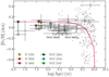 |
Fig. 11 Age-metallicity distribution for the YOCs we analysed here, for the sample of Netopil et al. (2016) (empty circles), field stars taken from Bensby et al. (2014) (grey crosses), and Gaia-ESO clusters analysed in Magrini et al. (2018) (filled triangles). The red line represents the model by Minchev et al. (2013) for 7.5 < RGal < 9 kpc. See text for further details. The empty stars represent the clusters we analysed whose metallicity was derived with the standard analysis (Netopil et al. 2016). |
Acknowledgements
We thank the anonymous referee for very helpful comments and suggestions. This work is based on data products from observations made with ESO Telescopes at the La Silla Paranal Observatory under programme ID 188.B-3002. These data products have been processed by the Cambridge Astronomy Survey Unit (CASU) at the Institute of Astronomy, University of Cambridge, and by the FLAMES/UVES reduction team at INAF/Osservatorio Astrofisico di Arcetri. These data have been obtained from the Gaia-ESO Survey Data Archive, prepared and hosted by the Wide Field Astronomy Unit, Institute for Astronomy, University of Edinburgh, which is funded by the UK Science and Technology Facilities Council. This work was partly supported by the European Union FP7 programme through ERC grant number 320360 and by the Leverhulme Trust through grant RPG-2012-541. We acknowledge the support from INAF and Ministero dell’ Istruzione, dell’ Università’ e della Ricerca (MIUR) in the form of the grant “Premiale VLT 2012”. The results presented here benefit from discussions held during the Gaia-ESO workshops and conferences supported by the ESF (European Science Foundation) through the GREAT Research Network Programme. V.A. is supported by FCT – Fundaçãopara a Ciência e a Tecnologia through national funds and by FEDER through COMPETE2020 – Programa Operacional Competitividade e Internacionalização by these grants: Investigador FCT contract nr. IF/00650/2015/CP1273/CT0001; UID/FIS/04434/2019; PTDC/FIS-AST/28953/2017 & POCI-01-0145-FEDER-028953 and PTDC/FIS-AST/32113/2017 & POCI-01-0145-FEDER-032113. F.J.E. acknowledges financial support from the Spanish MINECO/FEDER through grant AyA2017-84089. T.B. was supported by the project grant “The New Milky Way” from the Knut and Alice Wallenberg Foundation. U.H. acknowledges support from the Swedish National Space Agency (SNSA/Rymdstyrelsen). S.G.S acknowledges the support by Fundação para a Ciência e Tecnologia (FCT) through national funds and a research grant (project ref. UID/FIS/04434/2013, and PTDC/FIS-AST/7073/2014). S.G.S. also acknowledge the support from FCT through Investigador FCT contract of reference IF/00028/2014 and POPH/FSE (EC) by FEDER funding through the program – Programa Operacional de Factores de Competitividade – COMPETE.
Appendix A Additional tables
Different values of Teff derived with photometry, Fe lines alone, and Fe and Ti simultaneously.
Derived stellar parameters and abundances with the final models and comparison with the photometric values.
Abundance ratios for different species.
References
- Asplund, M., Grevesse, N., Sauval, A. J., & Scott, P. 2009, ARA&A, 47, 481 [NASA ADS] [CrossRef] [Google Scholar]
- Bailey, J. I., Mateo, M., White, R. J., Shectman, S. A., & Crane, J. D. 2018, MNRAS, 475, 1609 [NASA ADS] [CrossRef] [Google Scholar]
- Barklem, P. S., Piskunov, N., & O’Mara, B. J. 2000, A&AS, 142, 467 [NASA ADS] [CrossRef] [EDP Sciences] [MathSciNet] [PubMed] [Google Scholar]
- Barrado y Navascues, D., Stauffer, J. R., & Patten, B. M. 1999, ApJ, 522, L53 [NASA ADS] [CrossRef] [Google Scholar]
- Barrado y Navascués, D., Stauffer, J. R., & Jayawardhana, R. 2004, ApJ, 614, 386 [NASA ADS] [CrossRef] [Google Scholar]
- Bensby, T., Feltzing, S., & Oey, M. S. 2014, A&A, 562, A71 [NASA ADS] [CrossRef] [EDP Sciences] [Google Scholar]
- Bergemann, M. 2011, MNRAS, 413, 2184 [NASA ADS] [CrossRef] [Google Scholar]
- Biazzo, K., Randich, S., & Palla, F. 2011a, A&A, 525, A35 [NASA ADS] [CrossRef] [EDP Sciences] [Google Scholar]
- Biazzo, K., Randich, S., Palla, F., & Briceño, C. 2011b, A&A, 530, A19 [NASA ADS] [CrossRef] [EDP Sciences] [Google Scholar]
- Blanco-Cuaresma, S., Soubiran, C., Jofré, P., & Heiter, U. 2014, A&A, 566, A98 [NASA ADS] [CrossRef] [EDP Sciences] [Google Scholar]
- Cantat-Gaudin, T., Jordi, C., Vallenari, A., et al. 2018, A&A, 618, A93 [NASA ADS] [CrossRef] [EDP Sciences] [Google Scholar]
- Cargile, P. A., & James, D. J. 2010, AJ, 140, 677 [NASA ADS] [CrossRef] [Google Scholar]
- Carrera, R., Bragaglia, A., Cantat-Gaudin, T., et al. 2019, A&A, 623, A80 [NASA ADS] [CrossRef] [EDP Sciences] [Google Scholar]
- Casagrande, L., Ramírez, I., Meléndez, J., Bessell, M., & Asplund, M. 2010, A&A, 512, A54 [NASA ADS] [CrossRef] [EDP Sciences] [Google Scholar]
- Casamiquela, L., Blanco-Cuaresma, S., Carrera, R., et al. 2019, MNRAS, 490, 1821 [NASA ADS] [CrossRef] [Google Scholar]
- Chen, Y. Q., Zhao, G., Izumiura, H., et al. 2008, AJ, 135, 618 [NASA ADS] [CrossRef] [Google Scholar]
- Cunha, K., Frinchaboy, P. M., Souto, D., et al. 2016, Astron. Nachr., 337, 922 [NASA ADS] [CrossRef] [Google Scholar]
- Cutri, R. M., Skrutskie, M. F., van Dyk, S., et al. 2003, 2MASS All Sky Catalog of point sources [Google Scholar]
- Delgado Mena, E., Moya, A., Adibekyan, V., et al. 2019, A&A, 624, A78 [NASA ADS] [CrossRef] [EDP Sciences] [Google Scholar]
- De Silva, G. M., D’Orazi, V., Melo, C., et al. 2013, MNRAS, 431, 1005 [NASA ADS] [CrossRef] [Google Scholar]
- Donati, P., Bragaglia, A., Carretta, E., et al. 2015, MNRAS, 453, 4185 [NASA ADS] [CrossRef] [Google Scholar]
- Donor, J., Frinchaboy, P. M., Cunha, K., et al. 2018, AJ, 156, 142 [NASA ADS] [CrossRef] [Google Scholar]
- D’Orazi, V., & Randich, S. 2009, A&A, 501, 553 [NASA ADS] [CrossRef] [EDP Sciences] [Google Scholar]
- D’Orazi, V., Magrini, L., Randich, S., et al. 2009, ApJ, 693, L31 [NASA ADS] [CrossRef] [Google Scholar]
- D’Orazi, V., Biazzo, K., & Randich, S. 2011, A&A, 526, A103 [NASA ADS] [CrossRef] [EDP Sciences] [Google Scholar]
- D’Orazi, V., De Silva, G. M., & Melo, C. F. H. 2017a, A&A, 598, A86 [NASA ADS] [CrossRef] [EDP Sciences] [Google Scholar]
- D’Orazi, V., Desidera, S., Gratton, R. G., et al. 2017b, A&A, 598, A19 [NASA ADS] [CrossRef] [EDP Sciences] [Google Scholar]
- Folsom, C. P., Petit, P., Bouvier, J., et al. 2016, MNRAS, 457, 580 [NASA ADS] [CrossRef] [Google Scholar]
- Friel, E. D. 1995, ARA&A, 33, 381 [NASA ADS] [CrossRef] [Google Scholar]
- Froese Fischer, C., & Tachiev, G. 2012, Multiconfiguration Hartree-Fock and Multiconfiguration Dirac-Hartree-Fock Collection, Version 2, available at http://physics.nist.gov/mchf/ [Google Scholar]
- Galarza, J. Y., Meléndez, J., Lorenzo-Oliveira, D., et al. 2019, MNRAS, 490, L86 [NASA ADS] [CrossRef] [Google Scholar]
- Gilmore, G., Randich, S., Asplund, M., et al. 2012, The Messenger, 147, 25 [NASA ADS] [Google Scholar]
- Gurtovenko, E. A., & Sheminova, V. A. 2015, ArXiv e-prints [arXiv:1505.00975] [Google Scholar]
- Gustafsson, B., Edvardsson, B., Eriksson, K., et al. 2008, A&A, 486, 951 [NASA ADS] [CrossRef] [EDP Sciences] [Google Scholar]
- Heiter, U., Soubiran, C., Netopil, M., & Paunzen, E. 2014, A&A, 561, A93 [NASA ADS] [CrossRef] [EDP Sciences] [Google Scholar]
- Heiter, U., Lind, K., Bergemann, M., et al. 2019, A&A, submitted [Google Scholar]
- Jacobson, H. R., & Friel, E. D. 2013, AJ, 145, 107 [NASA ADS] [CrossRef] [Google Scholar]
- Jacobson, H. R., Friel, E. D., Jílková, L., et al. 2016, A&A, 591, A37 [NASA ADS] [CrossRef] [EDP Sciences] [Google Scholar]
- James, D. J., Melo, C., Santos, N. C., & Bouvier, J. 2006, A&A, 446, 971 [NASA ADS] [CrossRef] [EDP Sciences] [Google Scholar]
- Jofré, P., Heiter, U., Soubiran, C., et al. 2015, A&A, 582, A81 [NASA ADS] [CrossRef] [EDP Sciences] [Google Scholar]
- Jofré, P., Heiter, U., Tucci Maia, M., et al. 2018, Res. Notes AAS, 2, 152 [Google Scholar]
- King, J. R., Soderblom, D. R., Fischer, D., & Jones, B. F. 2000, ApJ, 533, 944 [NASA ADS] [CrossRef] [Google Scholar]
- Lanzafame, A.C., Frasca, A., Damiani, F., et al. 2015, A&A, 576, A80 [NASA ADS] [CrossRef] [EDP Sciences] [Google Scholar]
- Lawler, J. E., Guzman, A., Wood, M. P., Sneden, C., & Cowan, J. J. 2013, ApJS, 205, 11 [NASA ADS] [CrossRef] [Google Scholar]
- Lodders, K., Palme, H., & Gail, H. P. 2009, Solar System (Berlin: Springer), 4B, 712 [Google Scholar]
- Magrini, L., Randich, S., Kordopatis, G., et al. 2017, A&A, 603, A2 [NASA ADS] [CrossRef] [EDP Sciences] [Google Scholar]
- Magrini, L., Spina, L., Randich, S., et al. 2018, A&A, 617, A106 [NASA ADS] [CrossRef] [EDP Sciences] [Google Scholar]
- Maiorca, E., Randich, S., Busso, M., Magrini, L., & Palmerini, S. 2011, ApJ, 736, 120 [NASA ADS] [CrossRef] [Google Scholar]
- Maiorca, E., Magrini, L., Busso, M., et al. 2012, ApJ, 747, 53 [NASA ADS] [CrossRef] [Google Scholar]
- Mamajek, E. E., & Hillenbrand, L. A. 2008, ApJ, 687, 1264 [NASA ADS] [CrossRef] [Google Scholar]
- Marigo, P., Girardi, L., Bressan, A., et al. 2017, ApJ, 835, 77 [NASA ADS] [CrossRef] [Google Scholar]
- Masana, E., Jordi, C., & Ribas, I. 2006, A&A, 450, 735 [NASA ADS] [CrossRef] [EDP Sciences] [Google Scholar]
- Meléndez, J., Ramírez, I., Karakas, A. a. I., et al. 2014, ApJ, 791, 14 [NASA ADS] [CrossRef] [Google Scholar]
- Minchev, I., Chiappini, C., & Martig, M. 2013, A&A, 558, A9 [NASA ADS] [CrossRef] [EDP Sciences] [Google Scholar]
- Mishenina, T., Pignatari, M., Carraro, G., et al. 2015, MNRAS, 446, 3651 [NASA ADS] [CrossRef] [Google Scholar]
- Modigliani, A., Mulas, G., Porceddu, I., et al. 2004, The Messenger, 118, 8 [NASA ADS] [Google Scholar]
- Nayakshin, S. 2017, PASA, 34, e002 [NASA ADS] [CrossRef] [Google Scholar]
- Naylor, T., & Jeffries, R. D. 2006, MNRAS, 373, 1251 [NASA ADS] [CrossRef] [Google Scholar]
- Netopil, M., Paunzen, E., Heiter, U., & Soubiran, C. 2016, A&A, 585, A150 [NASA ADS] [CrossRef] [EDP Sciences] [Google Scholar]
- Origlia, L., Dalessandro, E., Sanna, N., et al. 2019, A&A, 629, A117 [NASA ADS] [CrossRef] [EDP Sciences] [Google Scholar]
- Pasquini, L., Avila, G., Blecha, A., et al. 2002, The Messenger, 110, 1 [Google Scholar]
- Pollack, J. B., Hubickyj, O., Bodenheimer, P., et al. 1996, Icarus, 124, 62 [NASA ADS] [CrossRef] [Google Scholar]
- Randich, S., Gilmore, G., & Gaia-ESO Consortium 2013, The Messenger, 154, 47 [NASA ADS] [Google Scholar]
- Reddy, A. B. S., & Lambert, D. L. 2015, MNRAS, 454, 1976 [NASA ADS] [CrossRef] [Google Scholar]
- Reddy, A. B. S., & Lambert, D. L. 2017, ApJ, 845, 151 [NASA ADS] [CrossRef] [Google Scholar]
- Reddy, A. B. S., Lambert, D. L., & Giridhar, S. 2016, MNRAS, 463, 4366 [NASA ADS] [CrossRef] [Google Scholar]
- Sacco, G. G., Morbidelli, L., Franciosini, E., et al. 2014, A&A, 565, A113 [NASA ADS] [CrossRef] [EDP Sciences] [Google Scholar]
- Samland, M., Mollière, P., Bonnefoy, M., et al. 2017, A&A, 603, A57 [NASA ADS] [CrossRef] [EDP Sciences] [Google Scholar]
- Santos, N. C., Israelian, G., & Mayor, M. 2003, in The Future of Cool-Star Astrophysics: 12th Cambridge Workshop on Cool Stars, Stellar Systems, and the Sun, eds. A. Brown, G. M. Harper, & T. R. Ayres (San Francisco: ASP), 12, 148 [NASA ADS] [Google Scholar]
- Santos, N. C., Melo, C., James, D. J., et al. 2008, A&A, 480, 889 [NASA ADS] [CrossRef] [EDP Sciences] [Google Scholar]
- Schuler, S. C., Plunkett, A. L., King, J. R., & Pinsonneault, M. H. 2010, PASP, 122, 766 [NASA ADS] [CrossRef] [Google Scholar]
- Shen, Z. X., Jones, B., Lin, D. N. C., Liu, X. W., & Li, S. L. 2005, ApJ, 635, 608 [NASA ADS] [CrossRef] [Google Scholar]
- Smiljanic, R., Korn, A. J., Bergemann, M., et al. 2014, A&A, 570, A122 [NASA ADS] [CrossRef] [EDP Sciences] [Google Scholar]
- Sneden, C. A. 1973, PhD Thesis, The University of Texas at Austin, USA [Google Scholar]
- Sobeck, J. S., Kraft, R. P., Sneden, C., et al. 2011, AJ, 141, 175 [NASA ADS] [CrossRef] [Google Scholar]
- Sousa, S. G., Santos, N. C., Adibekyan, V., Delgado-Mena, E., & Israelian, G. 2015, A&A, 577, A67 [NASA ADS] [CrossRef] [EDP Sciences] [Google Scholar]
- Spina, L., Randich, S., Palla, F., et al. 2014a, A&A, 568, A2 [NASA ADS] [CrossRef] [EDP Sciences] [Google Scholar]
- Spina, L., Randich, S., Palla, F., et al. 2014b, A&A, 567, A55 [NASA ADS] [CrossRef] [EDP Sciences] [Google Scholar]
- Spina, L., Randich, S., Magrini, L., et al. 2017, A&A, 601, A70 [NASA ADS] [CrossRef] [EDP Sciences] [Google Scholar]
- Sung, H., Bessell, M. S., & Chun, M.-Y. 2004, AJ, 128, 1684 [NASA ADS] [CrossRef] [Google Scholar]
- Terndrup, D. M., Pinsonneault, M., Jeffries, R. D., et al. 2002, ApJ, 576, 950 [NASA ADS] [CrossRef] [Google Scholar]
- Tsantaki, M., Santos, N. C., Sousa, S. G., et al. 2019, MNRAS, 485, 2772 [NASA ADS] [CrossRef] [Google Scholar]
- Turner, D. G. 2012, Astron. Nachr., 333, 174 [NASA ADS] [CrossRef] [Google Scholar]
- van Leeuwen, F. 2009, A&A, 497, 209 [NASA ADS] [CrossRef] [EDP Sciences] [Google Scholar]
- Venuti, L., Prisinzano, L., Sacco, G. G., et al. 2018, A&A, 609, A10 [NASA ADS] [CrossRef] [EDP Sciences] [Google Scholar]
- Viana Almeida, P., Santos, N. C., Melo, C., et al. 2009, A&A, 501, 965 [NASA ADS] [CrossRef] [EDP Sciences] [Google Scholar]
- Vigan, A., Bonnefoy, M., Ginski, C., et al. 2016, A&A, 587, A55 [NASA ADS] [CrossRef] [EDP Sciences] [Google Scholar]
All Tables
Solar abundances derived here and in Asplund et al. (2009, A09), and meteoritic abundances from Lodders et al. (2009, L09).
Different values of Teff derived with photometry, Fe lines alone, and Fe and Ti simultaneously.
Derived stellar parameters and abundances with the final models and comparison with the photometric values.
All Figures
|
Fig. 1 Examples of the synthesis of several Fe I lines of star 08365498−5308342 (v sin i = 9.88 km s−1, as the recommended value given in the iDR5) for which the observed profile is not fitted when we adopt the ξ value obtained from the Fe lines (ξ = 1.75 km s−1; red line) and with the values derived with the new method (ξ = 0.85 km s−1; blue line). |
| In the text | |
|
Fig. 2 Number of Ti I lines measured for each star as a function of S/N, colour-coded according to v sin i <20 km s−1. Stars with similar S/N but higher rotational velocities have fewer measurable lines. The number of Ti I lines measured in the Sun is reported in the top right corner. |
| In the text | |
|
Fig. 3 Example of applying the new method for star 08365498−5308342 (IC 2391, age 50 Myr). The green dots represent the Fe I lines, and the blue squares represent the Ti I lines; the red lines in both panels are the linear regression, and individual slope and uncertainties are reported for each panel. See text for further details. |
| In the text | |
|
Fig. 4 Comparison between the photometric and spectroscopic estimates of the atmospheric parameters. The red line represents the 1:1 relation. The points are colour-coded according to ages. The red points refer to NGC 2516, and the blue points to the younger clusters. |
| In the text | |
|
Fig. 5 Comparison between the values of Teff,spec, log gspec, ξspec, and [X/H] derived here with the values from Gaia-ESO iDR5. The red line represents the 1:1 relation. We exclude stars from the plot whose ξ value is fixed to the photometric estimates. See text for further details. |
| In the text | |
|
Fig. 6 [Fe/H] (top panel) and [Ti/H] (bottom panel) as a function of Teffderived using Fe and Ti lines simultaneously. For Fe, the Pearson correlation coefficient is r = 0.35, with p = 0.10, which is not significant at p < 0.05. For Ti, the Pearson correlation coefficient is r = 0.32, with p = 0.14, which is not significant at p < 0.05. |
| In the text | |
|
Fig. 7 [X/H] as function of Teff, derived with the new method and colour-coded according to age. |
| In the text | |
|
Fig. 8 [X/H] as function of log g, derived using only Ti lines and colour-coded according to age. |
| In the text | |
|
Fig. 9 Difference between the EWs of the Fe (black dots) and Ti (red dots) lines measured in the solar-analogue star 10442256−6415301 (30 Myr)and the Sun as a function of the optical depth of line formation log τ5000. The dot-dashed line is the trend for Fe lines. |
| In the text | |
|
Fig. 10 Activity index |
| In the text | |
|
Fig. 11 Age-metallicity distribution for the YOCs we analysed here, for the sample of Netopil et al. (2016) (empty circles), field stars taken from Bensby et al. (2014) (grey crosses), and Gaia-ESO clusters analysed in Magrini et al. (2018) (filled triangles). The red line represents the model by Minchev et al. (2013) for 7.5 < RGal < 9 kpc. See text for further details. The empty stars represent the clusters we analysed whose metallicity was derived with the standard analysis (Netopil et al. 2016). |
| In the text | |
Current usage metrics show cumulative count of Article Views (full-text article views including HTML views, PDF and ePub downloads, according to the available data) and Abstracts Views on Vision4Press platform.
Data correspond to usage on the plateform after 2015. The current usage metrics is available 48-96 hours after online publication and is updated daily on week days.
Initial download of the metrics may take a while.