| Issue |
A&A
Volume 634, February 2020
|
|
|---|---|---|
| Article Number | A89 | |
| Number of page(s) | 6 | |
| Section | Stellar structure and evolution | |
| DOI | https://doi.org/10.1051/0004-6361/201937036 | |
| Published online | 12 February 2020 | |
First characterization of Swift J1845.7–0037 with NuSTAR
1
Institut für Astronomie und Astrophysik, Sand 1, 72076 Tübingen, Germany
e-mail: This email address is being protected from spambots. You need JavaScript enabled to view it.
2
Department of Physics and Astronomy, University of Turku, 20014 Turku, Finland
3
Space Research Institute of the Russian Academy of Sciences, Profsoyuznaya Str. 84/32, Moscow 117997, Russia
4
Moscow Institute of Physics and Technology, Moscow Region, Dolgoprudnyi, Russia
5
Key Laboratory for Particle Astrophysics, Institute of High Energy Physics, Chinese Academy of Sciences, 19B Yuquan Road, Beijing 100049, PR China
6
University of Chinese Academy of Sciences, Chinese Academy of Sciences, Beijing 100049, PR China
Received:
1
November
2019
Accepted:
15
January
2020
Abstract
The hard X-ray transient source Swift J1845.7–0037 was discovered in 2012 by Swift/BAT. However, at that time, no dedicated observations of the source were performed. In October 2019, the source became active again, and X-ray pulsations with a period of ∼199 s were detected with Swift/XRT. This triggered follow-up observations with NuSTAR. Here, we report on the timing and spectral analysis of the source properties using NuSTAR and Swift/XRT. The main goal was to confirm pulsations and search for possible cyclotron lines in the broadband spectrum of the source to probe its magnetic field. Despite highly significant pulsations with period of 207.379(2) s being detected, no evidence for a cyclotron line was found in the spectrum of the source. We therefore discuss the strength of the magnetic field based on the source flux and the detection of the transition to the “cold-disc” accretion regime during the 2012 outburst. Our conclusion is that the source is most likely a highly magnetized neutron star with B ≳ 1013 G at a large distance of d ∼ 10 kpc. The latter is consistent with the nondetection of a cyclotron line in the NuSTAR energy band.
Key words: accretion, accretion disks / magnetic fields / stars: individual: Swift J1845.7-0037 / X-rays: binaries
© ESO 2020
1. Introduction
X-ray pulsars are magnetized neutron stars accreting matter supplied by nondegenerate companions in binary systems. Captured matter is funneled by the magnetic field of a spinning neutron star to its polar areas, where the gravitational energy of the accretion flow is released in the form of pulsed X-ray emission. Mass transfer can occur in several ways, for example, as a result of Roche-lobe outflow by the companion, directly from its stellar wind, or, in case of Be donors, from the decretion disc of the donor (so-called Be X-ray binaries). In the latter case, transient behavior in an X-ray band associated with passages of the compact object through a relatively dense Be disc and evolution of the disc itself is observed in most cases (Reig 2011). As a consequence, most of Be X-ray binaries (BeXRBs) are discovered during bright X-ray outbursts when accretion luminosity increases by up to five orders of magnitude (Doroshenko et al. 2019), and a large fraction of BeXRB population likely remains undetected (Doroshenko et al. 2014).
On the other hand, in outbursts, BeXRBs are usually among the brightest sources in X-ray sky, so a detailed analysis of their spectral and timing properties becomes feasible. In particular, many BeXRBs exhibit so-called cyclotron lines, or cyclotron resonance scattering features (CRSFs; Trümper et al. 1977) in their X-ray spectra. Detection of such an absorption feature in the spectrum of the X-ray pulsar enables the direct measurement of the magnetic field in a line-forming region because its energy is directly linked to the magnetic field strength, as Ecyc ∼ 11.57(B/1012) G (Staubert et al. 2019). Detection of CRSFs is, however, often challenging, due to the complex continuum spectrum shapes and lack of photons at higher energies, so other, indirect, estimates of the magnetic field are often invoked (Tsygankov et al. 2017a,b, 2016a). This is particularly relevant for stronger magnetized sources where the cyclotron line energy is too high to be detectable, and direct estimates of the field are not possible (Tsygankov et al. 2017a; Doroshenko et al. 2019).
The transient source Swift J1845.7–0037 was discovered in the XMM slew survey as XMMSL1 J184555.4−003941 (Saxton et al. 2008), and was later identified as a hard X-ray transient following the detection by Swift/BAT in 2012 (Krimm et al. 2012). In 2019, the source was detected by MAXI (Negoro et al. 2019) and followed-up by Swift/XRT, which allowed the detection of pulsations at ∼200 s (Kennea et al. 2019a) and better constrained the X-ray position of the source, thereby suggesting 2MASS J18455462−0039341 as an optical counterpart candidate (Steele 2019; Kennea 2019). Kennea et al. (2019a) also reported detection of pulsations in reanalyzed 2012 XRT data, which previously escaped detection due to the relatively long spin period of the source and short duration of the observations. An analysis of the spectral energy distribution of this object suggests it is a strongly absorbed early-type star with Teff ∼ 28 000−33 000 K (McCollum & Laine 2019a,b), consistent with the expected Be-transient origin of the source (Kennea et al. 2019a). Here, we report results of the follow-up observations of Swift J1845.7–0037 with the NuSTAR observatory (Harrison et al. 2013), which, firstly, aimed to provide characterization of its broadband X-ray properties.
2. Observations and data analysis
Following the detection of pulsations with MAXI (Kennea et al. 2019a), we triggered an observation of Swift J1845.7–0037 with NuSTAR on MJD 58777 for 44 ks (Obsid. 90501347002, effective exposure ∼23.5 ks). Data reduction was carried out using the HEASOFT 6.26.1 package with current calibration files (CALDB version 20191008) and standard data reduction procedures as described in the instruments documentation. Source spectra were extracted from a region of 54″ radius around the position of Swift J1845.7–0037, whereas background spectra were extracted from a circular region of 147″ radius away from the source. The extraction regions were optimized to increase the signal-to-noise ratio in the hard energy band ≥40 keV as described in Vybornov et al. (2018). The spectra for the two NuSTAR modules (FPMA and FPMB) were extracted independently and modeled simultaneously in the 3−79 keV range. All spectra were grouped to include at least 25 counts per energy bin. Light curves of the two modules were co-added and background subtracted unless stated otherwise. We also analyzed Swift/XRT observations, for which the source spectrum was extracted using online tools1 provided by the UK Swift Science Data Centre (Evans et al. 2009). The spectrum was grouped to contain at least 25 counts per energy bin and modeled simultaneously with the NuSTAR spectra using the XSPEC 12.10.1.f package (Arnaud et al. 1996).
2.1. Timing analysis
As shown in Fig. 1, strong pulsations with a period of ∼200 s are clearly visible directly in the source light curve. An epoch folding search reveals a strong peak around 207.4 s. We assumed the source position reported by Kennea et al. (2019a) for the barycentric correction. No binary correction was applied, as the orbital parameters are not known. To refine this value and estimate the uncertainty of the measured spin period, we used a phase-connection technique (Deeter et al. 1981). Times of arrival (TOAs) of individual pulse cycles were determined by directly fitting the average template obtained by folding the entire 3–20 keV light curve with the period found above to lightcurve. The average uncertainty of TOAs was found to be ∼1.7 s. The individual TOAs were then fitted assuming a constant period, that is, ti, calc = ni × p + t0, which resulted in the period estimate of P = 207.379(2) (all uncertainties are quoted at 1σ confidence level). No evidence for the change of the spin period within the observation was found, which is not surprising considering its relatively short duration.
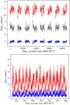 |
Fig. 1. Light curve of the source as observed by NuSTAR in 3–10 keV (red) and 20–40 keV (blue) bands (top, both units combined, one bin per pulse), and the ratio of the two (black points). Bottom panel: part of the light curve of the source in the 3–10 keV (red) and 20–40 keV (blue) bands. Strong pulsations with a period of ∼200 s are observed throughout the full energy range. |
Using the obtained period, we folded the light curves extracted in several energy bands in order to investigate the evolution of the pulse profile with the energy. As shown in Fig. 2, the pulse profile at lower energies exhibits a complex morphology, showing several narrower peaks within a broader main peak and its rising phase. At higher energies (≳15 keV), these structures gradually disappear. This can be better illustrated with the phase-energy matrix shown in the same figure. In addition, the pulsed fraction decreases with the energy at soft X-rays, whereas it increases in hard bands, reaching almost 90% at the highest energies (Fig. 3), as is typical for bright X-ray pulsars (Lutovinov & Tsygankov 2009). We note that the uncertainties for the pulsed fraction were estimated assuming normal distribution of counts in individual phase bins, which is not the case for the highest energy bins, so the uncertainties there are likely overestimated.
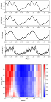 |
Fig. 2. Representative pulse profiles of source normalized by dividing by the average source intensity in the frame using efold task as observed by NuSTAR in several energy bands (top), and the phase-energy matrix showing the energy evolution of the (normalized) pulse profiles in details (bottom). In the latter case, slices along the constant energy represent normalized pulse profiles similar to those shown in the top panel. We note the energy dependence of pulse profile shape, particularly around ∼15 keV. |
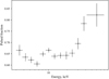 |
Fig. 3. Pulsed fraction of Swift J1845.7–0037 defined as (max(rate)−min(rate))/((max(rate)+min(rate)) as a function of the energy. |
We note that the observed pulse profile evolution suggests a possible presence of an independent soft spectral component, which exhibits a different and more complex dependence on the pulse phase.
2.2. Spectral analysis
As reported by Doroshenko & Tsygankov (2019), the source spectrum measured with NuSTAR is typical of X-ray pulsars and can be described with a Comptonization model with an electron temperature of 6−7 keV. It does not show any evident absorption features suggestive of electron CRSFs. This conclusion does not depend on the model chosen to describe the continuum emission. The latter can be described by different continuum models, such as a cutoff power law combined with partial-covering absorption, or an additional soft blackbody component, a combination of different Comptonization models, etc. Considering that the interpretation of parameters of commonly used phenomenological models is often rather ambiguous, here we adopt one of the simplest commonly used models adequately describing the broadband phase-averaged spectrum of the source. This is an absorbed power law with the Fermi-Dirac (Tanaka et al. 1986) cutoff implemented using the mdefine command in the XSPEC package. The absorption was modeled using TBabs model and abundances from Wilms et al. (2000). Besides the continuum, we also included in the model a narrow Gaussian line at ∼6.4 keV to account for the weak iron line observed in the spectrum of the source, and cross-normalization constants to account for slight differences in the absolute flux between two NuSTAR telescope modules and Swift/XRT.
For the phase-averaged analysis we used only a single XRT observation (Obsid. 00032472018), the closest in time to the NuSTAR observation. In fact, Swift observed the source on MJD 58775.5 whereas the NuSTAR observation started 1.5 days later. This resulted in a much lower exposure (∼750 s) and counting statistics in the soft energy band. Still, extending the lower energy coverage helped to constrain the absorption column which appears to be a factor of two higher compared to the expected interstellar value (∼1.72 × 10²² atoms cm−2; HI4PI Collaboration 2016).
As already mentioned, best-fit residuals with fdcut model reveal no evidence for any absorption features (see, i.e., Fig. 4). Still, we performed a search for possible CRSFs through the inclusion of a multiplicative Gaussian absorption line (gabs in Xspec) with arbitrary fixed energy in the fit (in addition to the best-fit model described above). Considering that the widths of observed CRSFs have been reported to correlate with centroid energy (Coburn et al. 2002; Doroshenko 2017), we fixed the width of the line to σ = 0.12Ecyc + 0.8 as reported by Doroshenko (2017)2 for this search. We found that for all energies, the depth of the line was consistent with zero at 3σ confidence level, with the upper limit on possible line depth ranging from 0.07 to 40 as presented in Fig. 5. We note that for energies below ∼40 keV, this is lower than for most other pulsars where CRSF has been robustly detected (Staubert et al. 2019). Moreover, the significance of this additional feature as estimated using the f-test is also comparatively low for all energies (≤2.4σ).
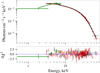 |
Fig. 4. Unfolded spectrum assuming best-fit FDCUT continuum as observed by Swift/XRT (green), and NuSTAR (black for FPMA and red for FPMB). The lower panel shows corresponding residuals. |
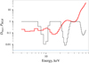 |
Fig. 5. Upper limit for depth of the potential CRSF (red) and corresponding f-test chance probability of fit improvement (black) as function of energy. The thin horizontal line indicates a 3σ confidence level for line detection. |
The largest statistical improvement from the inclusion of the feature appears for energy ∼29 keV, where the fit statistics further improve from 564.51 (for 580 degrees of freedom) to 554.70 (for 577 degrees of freedom) when line width is also allowed to vary (in which case, it becomes ∼9 keV). This improvement corresponds to a chance improvement probability of ∼2% (or ∼2σ according to f-test), making it not really significant. Considering that the f-test is, strictly speaking, inapplicable when testing for the presence of line-like features (Protassov et al. 2002), we also estimated the significance of the potential CRSF at this energy using the approach outlined by Bodaghee et al. (2016).
In particular, using the simftest script (included as part of Xspec), we simulated 2000 spectra with the same binning and same counting statistics as real data based on the best-fit model with no feature included (i.e., containing no line). Simulated spectra were then fit using the best-fit models, both with and without inclusion of the line at ∼29 keV (corresponding to deepest potential feature found in blind search). For each fit, we noted the change in Δχ2 associated with inclusion of the additional model component (i.e., CRSF). In approximately half of the realizations, the fit statistics were not improved when a more complex model was realized, and in ∼2% of realizations where the fit did improve, the improvement turned out to be equal to, or greater than, the observed value (i.e., 10.87), which suggests that observed improvement is quite likely due to statistical fluctuations in the data. The resulting distribution of obtained Δχ2 is presented in Fig. 6, and, as expected, follows the χ2 distribution for three degrees of freedom (inclusion of the line adds three free parameters). This allows to estimate the chance probability of the observed fit improvement, which turns out to be ∼1.2% and implies line significance of ∼2.2σ. We conclude, therefore, that there is no strong evidence for the presence of a CRSF in spectrum of the source.
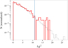 |
Fig. 6. Distribution of obtained fit improvements (Δχ2) when fitting simulated spectra including no line with a model including the line (red). The expected chance improvement (for χ2 distribution with three degrees of freedom) is also plotted for reference (black dots). The largest improvement obtained from the observed data (10.87) is indicated by a vertical line and corresponds to a chance probability of ∼1.2%. |
The best-fit parameters for the continuum component and the iron line are listed in Table 1. In addition, the table includes the values of the cross-normalization constants, and the observed and unabsorbed fluxes in the 0.1–100 keV energy band.
Best-fit parameters of the phase-averaged spectrum of Swift J1845.7–0037 using the FDCUT model.
We also performed pulse-phase resolved spectral analysis using the model described above. The number of phase bins (10) was chosen considering the typical width of structures observed in soft pulse profile (∼0.1 of phase as illustrated in Fig. 2), and at the same time to maintain reasonable accuracy for the derived spectral parameters. The zero phase was selected to ensure that the variations of the ratio between soft and hard pulse profiles are approximately aligned with phase-bin boundaries. Considering that Swift/XRT data could not be used, we fixed the absorption column and iron line parameters to values derived from the phase-averaged spectral analysis (after verifying that there is no significant variation). Variations of the remaining parameters with the pulse phase are shown in Fig. 7.
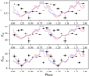 |
Fig. 7. Evolution ofFDCUT continuum parameters with the pulse phase. The pulse profiles of the source in soft (3–20 keV, red) and hard (20–80 keV, blue) are also plotted for reference. |
3. Discussion and summary
The transient source Swift J1845.7–0037 was discovered in 2012. No dedicated observations in the broad energy band were performed, and the source was only observed by all sky monitors and Swift/XRT. In October 2019, a new outburst from the source was observed by MAXI (Kennea et al. 2019b), which was followed-up firstly with Swift, which provided hints for pulsations (Kennea et al. 2019a), and then with NuSTAR. We observed the source on Oct 21, 2019, confirming strong pulsations with high significance. Besides confirming the nature of the source, one of the prime goals of our investigation was to search for possible electron CRSFs in the spectrum to estimate the strength of the pulsar’s magnetic field. Unfortunately, our analysis did not show substantial evidence for cyclotron lines. In fact, the broadband continuum spectrum of the source can be well-described by different phenomenological models without the necessity to include any absorption line in any of the models. The source’s spin period remained constant, which, together with the unknown orbit and distance, precludes any estimate of the magnetic field by modeling spin evolution with accretion torque models (see, e.g., Tsygankov et al. 2016b, 2017a; Doroshenko et al. 2018; Lutovinov et al. 2019, for the current results).
Still, important information on the source properties has been deduced based the X-ray phenomenology. First of all, comparison of the observed source flux with typical peak luminosities (∼5 × 1036−1037 erg s−1) reached in outbursts by other Be transients, suggests comparatively large distance to the source ∼5−10 kpc, and larger if current detection occurred during a type II outburst, where the luminosity can be up to two orders of magnitude higher. This conclusion is consistent with the observed strong absorption both in the X-ray (see Table 1) and optical bands (McCollum & Laine 2019b). We note that strong local absorption is not common for BeXRBs (even if it can not be ruled out), and the observed value exceeds the expected interstellar absorption integrated over the entire Galaxy, which points to large distance to the source.
We note that this conclusion is also in line with the observed complex energy evolution of the pulse profile and observed variation of spectral parameters with the pulse phase (Karino 2007). Indeed, strong energy dependence of the pulse profiles suggests a strong energy dependence of the intrinsic beam pattern, as is expected for high luminosity accreting pulsars, where an accretion column is expected to develop (Basko & Sunyaev 1976). On the contrary, pulse profiles of complex morphology and energy dependence are not normally observed in accreting pulsars of lower luminosity (∼5 × 1036 erg s−1, Karino 2007), although there are also exceptions.
The complex phase dependence of the source spectrum at high luminosities can be explained by the phase-dependent visibility of different regions of the column and of parts of the neutron star’s surface illuminated by the column (Kraus et al. 2003; Poutanen et al. 2013). We emphasize that any meaningful interpretation of the observed variations of spectra parameters of the phenomenological models like FDCUT is not straightforward, especially considering that the observed pulse profile evolution with the energy suggests a combination of emission components from the two poles of the pulsar, which may contribute to the spectrum at any phase, although with a different weight. Still, one might notice that the variation of the photon index Γ and folding energy Efold follows different patterns. While the latter traces the overall flux evolution, the former is phase-shifted by ∼0.25. This could again point to the presence of two independent spectral components with a similar visibility pattern throughout the pulse, but shifted in phase, meaning the emission from two poles of the pulsar. This conclusion could be confirmed by the detailed modeling of the pulse profiles similar to that performed by Kraus et al. (2003), which is, however, out of the scope of the current work. Nevertheless, the complex phase dependence of spectral parameters again points to the presence of an accretion column in Swift J1845.7–0037, which then implies a super-critical luminosity of ∼1037 erg s−1 (Basko & Sunyaev 1976). We note that this value depends only weakly on the assumed magnetic field strength of the neutron star unless it is magnetar-like (Mushtukov et al. 2015). Comparing this luminosity with the observed flux yields a distance of ∼10 kpc, in agreement with other considerations discussed above. We emphasize that, similarly to other considerations above, this is a very rough estimate, and a much more robust distance estimate can hopefully be obtained from follow-up observations of the counterpart.
The magnetic field of the source cannot be directly estimated, due to the lack of detection of any CRSFs. Nevertheless, some indirect estimates can be made based on the analysis of archival Swift/XRT data from the 2012 outburst. To estimate the bolometric source flux, we extracted spectra of each XRT observation and fitted them using the same model used for the NuSTAR observations considering only the 0.5–10 keV flux as a free parameter (i.e., multiplied the model by the cflux component). Here, we used XRT data in the 0.5–10 keV and 0.9–10 keV bands for the photon counting and windowed modes, respectively. Spectra were grouped to contain at least one count per energy bin. We used lstat to fit the spectra and estimate the flux uncertainties. The obtained fluxes were then multiplied by the bolometric correction of 4.96 estimated from the NuSTAR fit to get an unabsorbed source flux in the 0.1–100 keV energy band. The resulting light curve of the declining tail of the 2012 outburst is shown in Fig. 8. The flux in the decay of the outburst levels out around MJD 56090 at FX ∼ 2 × 10⁻¹¹ erg cm−2 s−1 (note the logarithmic scale for flux), which is strikingly similar to the behavior observed in several other pulsars (Tsygankov et al. 2017b, 2019).
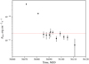 |
Fig. 8. Bolometric source flux estimated based on historic Swift/XRT light curve of the source as described in the text. The horizontal line indicates flux corresponding to transition to “cold”-disc accretion regime. |
In particular, Tsygankov et al. (2017b) argued that the flattening of the accretion rate at low fluxes observed in GRO J1008−57 is attributed to the transition of the accretion disc to the nonionized state with the lower viscosity, a well-known mechanism in dwarf novae. The transition luminosity is defined by the temperature at the inner boundary of the accretion disc, which, for magnetized objects, is in turn defined by the magnetic field strength:

Here, M1.4, R6, and B12 are neutron star mass in units of 1.4 M⊙, 106 cm, and 1012 G, respectively, and k ≃ 0.5 is the coupling constant defining the effective magnetospheric radius with respect to the classical Alfvén radius. As discussed by Tsygankov et al. (2017b), this estimate is rather crude, and depends on a number of assumptions, however, the scenario itself seems now to be confirmed by observations of the same state in several objects (Tsygankov et al. 2017b, 2019). We emphasize that, as discussed by Tsygankov et al. (2017b), the transition to the cold-disc state is actually inevitable for slowly spinning pulsars with P ≳ 40 s. We therefore suggest that the observed flux leveling in Swift J1845.7–0037 corresponds to this transition, which can be used to estimate its magnetic field.
As already mentioned, the flux corresponding to the transition in Swift J1845.7–0037 is FX ∼ 2 × 10⁻¹¹ erg cm−2 s−1, implying a luminosity of ∼2.4 × 1035(d/10 kpc)2 erg s−1, which can be compared either with the theoretical value, or observed transitional luminosity in the pulsar with the known field. In particular, in the source GRO J1008−57, such a transition occurs at ∼2 × 1035 erg s−1, and the field strength is estimated at 8 × 10¹² G (Yamamoto et al. 2013) based on the observed CRSF energy. We emphasize that the strong absorption, arguments on the source luminosity, and the pulse profile energy dependence all point to a large distance to the source (i.e., ∼10 kpc as assumed above), which implies that the magnetic field in Swift J1845.7–0037 must also be comparable to that in GRO J1008−57, i.e., around ∼1013 G. This translates to a rather high value of the cyclotron line energy at ≳80 keV, beyond the observational range of NuSTAR, and might explain nondetection of the line. We note that this argument can also be reversed, meaning one could argue that nondetection of the line, together with observed transition flux to a cold-disc accretion regime, suggests a large distance (∼10 kpc), which is a prediction that could hopefully be tested by follow-up optical observations.
Finally, we note that Insight-HXMT covering a broader energy range 1–250 keV (Li 2007; Zhang et al. 2019) have also observed the source seven times between MJD 58773 to 58776 for 150 ks in total at the flux of (1.3−1.7) × 10−9 erg cm−2 s−1, slightly higher than what was observed by NuSTAR. However, even then the source turned out to be too faint for the spectral analysis at hard X-rays. The timing analysis is ongoing and is to be published elsewhere. We emphasize, however, that the source would be the first priority for HXMT, INTEGRAL, and Swift/BAT whenever it undergoes a brighter outburst, as these are currently the only missions capable of testing presence of a cyclotron lines in the ≥80 keV energy band.
Acknowledgments
This research has made use of data and/or software provided by the High Energy Astrophysics Science Archive Research Center (HEASARC), which is a service of the Astrophysics Science Division at NASA/GSFC and the High Energy Astrophysics Division of the Smithsonian Astrophysical Observatory. This work made use of data supplied by the UK Swift Science Data Centre at the University of Leicester. Authors thank the Russian Science Foundation (grant 19-12-00423), National Natural Science Foundation of China (NSFC U1838201), German Academic Exchange Service (DAAD, project 57405000, VD), and the Academy of Finland travel grants 324550 (ST) and 316932 (AL) for support.
References
- Arnaud, K. A. 1996, in Astronomical Data Analysis Software and Systems V, eds. G. H. Jacoby, & J. Barnes, ASP Conf. Ser., 101, 17 [NASA ADS] [Google Scholar]
- Basko, M. M., & Sunyaev, R. A. 1976, MNRAS, 175, 395 [NASA ADS] [CrossRef] [Google Scholar]
- Bodaghee, A., Tomsick, J. A., Fornasini, F. M., et al. 2016, ApJ, 823, 146 [NASA ADS] [CrossRef] [Google Scholar]
- Coburn, W., Heindl, W. A., Rothschild, R. E., et al. 2002, ApJ, 580, 394 [NASA ADS] [CrossRef] [Google Scholar]
- Deeter, J. E., Boynton, P. E., & Pravdo, S. H. 1981, ApJ, 247, 1003 [NASA ADS] [CrossRef] [Google Scholar]
- Doroshenko, R. 2017, PhD Thesis, University of Tuebingen [Google Scholar]
- Doroshenko, V., & Tsygankov, S. 2019, The Astronomer’s Telegram, 13208 [Google Scholar]
- Doroshenko, V., Ducci, L., Santangelo, A., & Sasaki, M. 2014, A&A, 567, A7 [NASA ADS] [CrossRef] [EDP Sciences] [Google Scholar]
- Doroshenko, V., Tsygankov, S., & Santangelo, A. 2018, A&A, 613, A19 [NASA ADS] [CrossRef] [EDP Sciences] [Google Scholar]
- Doroshenko, V., Zhang, S. N., Santangelo, A., et al. 2019, MNRAS, 422, 2510 [Google Scholar]
- Evans, P. A., Beardmore, A. P., Page, K. L., et al. 2009, MNRAS, 397, 1177 [NASA ADS] [CrossRef] [Google Scholar]
- Harrison, F. A., Craig, W. W., Christensen, F. E., et al. 2013, ApJ, 770, 103 [NASA ADS] [CrossRef] [Google Scholar]
- HI4PI Collaboration (Ben Bekhti, N., et al.) 2016, A&A, 594, A116 [NASA ADS] [CrossRef] [EDP Sciences] [Google Scholar]
- Karino, S. 2007, PASJ, 59, 961 [NASA ADS] [Google Scholar]
- Kennea, J. 2019, ATel [Google Scholar]
- Kennea, J. A., Evans, P. A., Beardmore, A. P., et al. 2019a, ATel, 13195, 1 [NASA ADS] [Google Scholar]
- Kennea, J. A., Evans, P. A., Beardmore, A. P., et al. 2019b, ATel, 13191, 1 [NASA ADS] [Google Scholar]
- Kraus, U., Zahn, C., Weth, C., & Ruder, H. 2003, ApJ, 590, 424 [NASA ADS] [CrossRef] [Google Scholar]
- Krimm, H. A., Kennea, J. A., Holland, S. T., et al. 2012, ATel, 4130 [Google Scholar]
- Li, T.-P. 2007, Nucl. Phys. B Proc. Suppl., 166, 131 [NASA ADS] [CrossRef] [Google Scholar]
- Lutovinov, A. A., & Tsygankov, S. S. 2009, Astron. Lett., 35, 433 [NASA ADS] [CrossRef] [Google Scholar]
- Lutovinov, A. A., Tsygankov, S. S., Karasev, D. I., Molkov, S. V., & Doroshenko, V. 2019, MNRAS, 485, 770 [NASA ADS] [CrossRef] [Google Scholar]
- McCollum, B., & Laine, S. 2019a, The Astronomer’s Telegram, 13211, 1 [NASA ADS] [Google Scholar]
- McCollum, B., & Laine, S. 2019b, The Astronomer’s Telegram, 13222, 1 [NASA ADS] [Google Scholar]
- Mushtukov, A. A., Suleimanov, V. F., Tsygankov, S. S., & Poutanen, J. 2015, MNRAS, 447, 1847 [NASA ADS] [CrossRef] [Google Scholar]
- Negoro, H., Yoneyama, T., Serino, M., et al. 2019, ATel, 13189 [Google Scholar]
- Poutanen, J., Mushtukov, A. A., Suleimanov, V. F., et al. 2013, ApJ, 777, 115 [NASA ADS] [CrossRef] [Google Scholar]
- Protassov, R., van Dyk, D. A., Connors, A., Kashyap, V. L., & Siemiginowska, A. 2002, ApJ, 571, 545 [NASA ADS] [CrossRef] [Google Scholar]
- Reig, P. 2011, Ap&SS, 332, 1 [NASA ADS] [CrossRef] [Google Scholar]
- Saxton, R. D., Read, A. M., Esquej, P., et al. 2008, A&A, 480, 611 [NASA ADS] [CrossRef] [EDP Sciences] [Google Scholar]
- Staubert, R., Trümper, J., Kendziorra, E., et al. 2019, A&A, 622, A61 [NASA ADS] [CrossRef] [EDP Sciences] [Google Scholar]
- Steele, I. A. 2019, The Astronomer’s Telegram, 13218, 1 [NASA ADS] [Google Scholar]
- Tanaka, Y. 1986, in IAU Colloq. 89: Radiation Hydrodynamics in Stars and Compact Objects, eds. D. Mihalas, & K. H. A. Winkler (Berlin: Springer Verlag), Lecture Notes in Physics, 255, 198 [NASA ADS] [CrossRef] [Google Scholar]
- Trümper, J., Pietsch, W., Reppin, C., & Sacco, B. 1977, in Eighth Texas Symposium on Relativistic Astrophysics, M. D. Papagiannis, 302, 538 [Google Scholar]
- Tsygankov, S. S., Mushtukov, A. A., Suleimanov, V. F., & Poutanen, J. 2016a, MNRAS, 457, 1101 [NASA ADS] [CrossRef] [Google Scholar]
- Tsygankov, S. S., Lutovinov, A. A., Doroshenko, V., et al. 2016b, A&A, 593, A16 [NASA ADS] [CrossRef] [EDP Sciences] [Google Scholar]
- Tsygankov, S. S., Doroshenko, V., Lutovinov, A. A., Mushtukov, A. A., & Poutanen, J. 2017a, A&A, 605, A39 [NASA ADS] [CrossRef] [EDP Sciences] [Google Scholar]
- Tsygankov, S. S., Mushtukov, A. A., Suleimanov, V. F., et al. 2017b, A&A, 608, A17 [NASA ADS] [CrossRef] [EDP Sciences] [Google Scholar]
- Tsygankov, S. S., Doroshenko, V., Mushtukov, A. A., Lutovinov, A. A., & Poutanen, J. 2019, A&A, 621, A134 [NASA ADS] [CrossRef] [EDP Sciences] [Google Scholar]
- Vybornov, V., Doroshenko, V., Staubert, R., & Santangelo, A. 2018, A&A, 610, A88 [NASA ADS] [CrossRef] [EDP Sciences] [Google Scholar]
- Wilms, J., Allen, A., & McCray, R. 2000, ApJ, 542, 914 [NASA ADS] [CrossRef] [Google Scholar]
- Yamamoto, T., Mihara, T., Sugizaki, M., et al. 2013, ATel, 4759, 1 [NASA ADS] [Google Scholar]
- Zhang, S., Li, T., Lu, F., et al. 2019, ArXiv e-prints [arXiv:1910.09613] [Google Scholar]
All Tables
Best-fit parameters of the phase-averaged spectrum of Swift J1845.7–0037 using the FDCUT model.
All Figures
|
Fig. 1. Light curve of the source as observed by NuSTAR in 3–10 keV (red) and 20–40 keV (blue) bands (top, both units combined, one bin per pulse), and the ratio of the two (black points). Bottom panel: part of the light curve of the source in the 3–10 keV (red) and 20–40 keV (blue) bands. Strong pulsations with a period of ∼200 s are observed throughout the full energy range. |
| In the text | |
|
Fig. 2. Representative pulse profiles of source normalized by dividing by the average source intensity in the frame using efold task as observed by NuSTAR in several energy bands (top), and the phase-energy matrix showing the energy evolution of the (normalized) pulse profiles in details (bottom). In the latter case, slices along the constant energy represent normalized pulse profiles similar to those shown in the top panel. We note the energy dependence of pulse profile shape, particularly around ∼15 keV. |
| In the text | |
|
Fig. 3. Pulsed fraction of Swift J1845.7–0037 defined as (max(rate)−min(rate))/((max(rate)+min(rate)) as a function of the energy. |
| In the text | |
|
Fig. 4. Unfolded spectrum assuming best-fit FDCUT continuum as observed by Swift/XRT (green), and NuSTAR (black for FPMA and red for FPMB). The lower panel shows corresponding residuals. |
| In the text | |
|
Fig. 5. Upper limit for depth of the potential CRSF (red) and corresponding f-test chance probability of fit improvement (black) as function of energy. The thin horizontal line indicates a 3σ confidence level for line detection. |
| In the text | |
|
Fig. 6. Distribution of obtained fit improvements (Δχ2) when fitting simulated spectra including no line with a model including the line (red). The expected chance improvement (for χ2 distribution with three degrees of freedom) is also plotted for reference (black dots). The largest improvement obtained from the observed data (10.87) is indicated by a vertical line and corresponds to a chance probability of ∼1.2%. |
| In the text | |
|
Fig. 7. Evolution ofFDCUT continuum parameters with the pulse phase. The pulse profiles of the source in soft (3–20 keV, red) and hard (20–80 keV, blue) are also plotted for reference. |
| In the text | |
|
Fig. 8. Bolometric source flux estimated based on historic Swift/XRT light curve of the source as described in the text. The horizontal line indicates flux corresponding to transition to “cold”-disc accretion regime. |
| In the text | |
Current usage metrics show cumulative count of Article Views (full-text article views including HTML views, PDF and ePub downloads, according to the available data) and Abstracts Views on Vision4Press platform.
Data correspond to usage on the plateform after 2015. The current usage metrics is available 48-96 hours after online publication and is updated daily on week days.
Initial download of the metrics may take a while.