| Issue |
A&A
Volume 634, February 2020
|
|
|---|---|---|
| Article Number | A21 | |
| Number of page(s) | 17 | |
| Section | Extragalactic astronomy | |
| DOI | https://doi.org/10.1051/0004-6361/201936619 | |
| Published online | 30 January 2020 | |
The Carnegie Supernova Project II
Early observations and progenitor constraints of the Type Ib supernova LSQ13abf⋆,⋆⋆
1
Department of Physics and Astronomy, Aarhus University, Ny Munkegade 120, 8000 Aarhus C, Denmark
e-mail: This email address is being protected from spambots. You need JavaScript enabled to view it.
2
Homer L. Dodge Department of Physics and Astronomy, University of Oklahoma, 440 W. Brooks, Rm 100, Norman, OK 73019-2061, USA
3
Carnegie Observatories, Las Campanas Observatory, Casilla 601, La Serena, Chile
4
The Oskar Klein Centre, Department of Astronomy, Stockholm University, AlbaNova 10691, Stockholm, Sweden
5
George P. and Cynthia Woods Mitchell Institute for Fundamental Physics and Astronomy, Texas A&M University, Department of Physics and Astronomy, College Station, TX 77843, USA
6
Konkoly Observatory, CSFK, Konkoly-Thege M. ut 15-17, Budapest, Hungary
7
Department of Optics and Quantum Electronics, University of Szeged, Dom ter 9, Szeged, Hungary
8
Department of Astronomy, University of Texas, 1 University Station C1400, Austin, TX 78712, USA
9
Department of Physics, Florida State University, Tallahassee, FL 32306, USA
10
Observatories of the Carnegie Institution for Science, 813 Santa Barbara St., Pasadena, CA 91101, USA
11
Instituto de Astrofısica de La Plata (IALP), CONICET, Paseo del bosque s/n, 1900 La Plata, Argentina
12
Facultad de Ciencias Astronómicas y Geofísicas (FCAG), Universidad Nacional de La Plata (UNLP), Paseo del bosque s/n, 1900 La Plata, Argentina
13
Kavli Institute for the Physics and Mathematics of the Universe, Todai Institutes for Advanced Study, University of Tokyo, 5-1-5 Kashiwanoha, Kashiwa, Chiba 277-8583, Japan
14
Departamento de Física Teórica y del Cosmos, Universidad de Granada, 18071 Granada, Spain
Received:
3
September
2019
Accepted:
12
November
2019
Abstract
Supernova LSQ13abf was discovered soon after explosion by the La Silla-QUEST Survey and then followed by the Carnegie Supernova Project II at its optical and near-IR wavelengths. Our analysis indicates that LSQ13abf was discovered within two days of explosion and its first ≈10 days of evolution reveal a B-band light curve with an abrupt drop in luminosity. Contemporaneously, the V-band light curve exhibits a rise towards a first peak and the r- and i-band light curves show no early peak. The early light-curve evolution of LSQ13abf is reminiscent of the post-explosion cooling phase observed in the Type Ib SN 2008D, and the similarity between the two objects extends over weeks. Spectroscopically, LSQ13abf also resembles SN 2008D, with P Cygni He I features that strengthen over several weeks. Spectral energy distributions are constructed from the broad-bandphotometry, a UVOIR light curve is constructed by fitting black-body (BB) functions, and the underlying BB-temperature and BB-radius profiles are estimated. Explosion parameters are estimated by simultaneously fitting an Arnett model to the UVOIR light curve and the velocity evolution derived from spectral features, and an in addition to a post-shock breakout cooling model to the first two epochs of the bolometric evolution. This combined model suggests an explosion energy of 1.27 ± 0.23 × 1051 ergs, in addition to a relatively high ejecta mass of 5.94 ± 1.10 M⊙, a 56Ni mass of 0.16 ± 0.02 M⊙, and a progenitor-star radius of 28.0 ± 7.5 R⊙. The ejecta mass suggests the origins of LSQ13abf lie with a > 25 M⊙ zero-age-main-sequence mass progenitor and its estimated radius is three times larger compared to the result obtained from the same analysis applied to observations of SN 2008D, and nine times larger compared to SN 1999ex. Alternatively, a comparison of hydrodynamical simulations of ≳20−25 M⊙ zero-age-main-sequence progenitors that evolve to pre-supernova envelope masses of ≲10 M⊙ and extended (∼100 R⊙) envelopes also broadly match the observations of LSQ13abf.
Key words: supernovae: individual: LSQ13abf / supernovae: individual: SN 1999ex / supernovae: individual: SN 2008D / supernovae: individual: iPTF13bvn / supernovae: general
This paper includes data gathered with the Nordic Optical Telescope at the Observatorio del Roque de los Muchachos, La Palma, Spain, and the Magellan 6.5 m Telescopes located at Las Campanas Observatory, Chile.
Photometry and spectra presented in this paper are available on WISeREP.
© ESO 2020
1. Introduction
Core-collapse (CC) supernovae (SNe) mark the demise of massive stars. The characteristics of their progenitor stars can be measured directly from deep, high-spatial resolution pre-explosion images (Smartt 2015), but more frequently, they are measured indirectly by modeling their SN emission. The observations of SNe at different temporal phases provides different insights on the nature of their progenitors. For example, late-phase observations enable us to peer into the deepest layers of the SN ejecta (e.g. Jerkstrand 2017), providing clues on potential asymmetries and, through spectral synthesis, an estimate of the zero-age-main-sequence (ZAMS) mass of the progenitor (e.g., Mazzali et al. 2017). Early-time observations, on the other hand, provide information on the SN explosion parameters, This includes the kinetic energy (EK) of the explosion, the ejecta mass (Mej), the amount of 56Ni synthesized during the explosion, and the level of mixing of the radioactive isotopes. Furthermore, if the observations begin in the hours to days after explosion and catch the cooling tail that follows shock breakout, it is possible to estimate the radius of the progenitor at the moment of its death (e.g., Rabinak & Waxman 2011).
With the advent of fast, non-targeted optical surveys, very early discoveries occur more frequently than in the past, revealing in some cases peculiar emission features related to the progenitor structure. Before the era of large surveys, SNe were typically observed in the optical while they rise to the main peak followed by a decline; however, it is becoming more common to observe an early peak at blue wavelengths prior to the rise to the main peak several weeks after the explosion. This early blue flux observed in CC SNe arises from the rapid cooling of the ejecta after shock breakout (e.g. Chevalier 1992; Chevalier & Fransson 2008). Capturing these ephemeral epochs offers an avenue to elucidate details on a number of physical processes. In addition to shock break out, other factors may also be at play that shape the early light curve. These include (i) the presence of any extended structure of the progenitor star (Bersten et al. 2013; Nakar & Piro 2014; Piro 2015), (ii) an excess of emission produced by shock interaction between the rapidly expanding SN ejecta with a companion (Kasen 2010), (iii) the distribution of radioactive material (Folatelli et al. 2006; Bersten et al. 2013; Noebauer et al. 2017; Taddia et al. 2018a), and (iv) emission from a magnetar (Kasen et al. 2016).
The most famous and well-studied SN 1987A was a hydrogen-rich, peculiar CC Type II SN that presented the first evidence of an early optical peak (Hamuy et al. 1988). This discovery was followed with the hydrogen-poor, stripped-envelope Type IIb SN 1993J, showing a prominent cooling tail post explosion (Richmond et al. 1994; Clocchiatti et al. 1995), and later by other Type IIb SNe, e.g., SN 2011dh (Arcavi et al. 2011), SN 2011fu (Morales-Garoffolo et al. 2015), and SN 2013df (Morales-Garoffolo et al. 2014). Even super-luminous SNe (SLSNe) have been documented to exhibit an early peak that can be as luminous as that of a normal SN before slowly rising to maximum brightness months later (e.g., Nicholl & Smartt 2016).
A small number of stripped-envelope (SE) SNe without hydrogen (Type Ib) and without helium (Type Ic) have also been observed at very early epochs with light curve excesses. Among them, the Type Ib/c SN 1999ex was the first with an early time cooling tail (Stritzinger et al. 2002), followed by the Type Ib SN 2008D that was discovered in the moments after explosion through the serendipitous X-ray detection (Soderberg et al. 2008; Modjaz et al. 2009; Malesani et al. 2009). Recently, iPTF13bvn is another example of a SN Ib with an early peak (Fremling et al. 2016).
A handful of SNe Ic-BL such as SN 2006aj (e.g., Sollerman et al. 2006), GRB-SN 2010bh (Cano et al. 2011), and SN 2013dk (D’Elia et al. 2015) were also observed with double peaks. These studies were followed with the discovery of the SN Ic 2013ge that showed an early peak in the ultraviolet (UV; Drout et al. 2016), and the SN Ic iPTF15dtg that was the first spectroscopically normal SN Ic with an early peak (Taddia et al. 2016). More recently, the ultra-stripped SN Ic iPTF14gqr was found to exhibit an early peak, perhaps related to shock-cooling emission from an extended helium envelope (De et al. 2018). Even more recently, ZTF18aalrxas was discovered just after explosion and reveals a rise to its first maximum (Fremling et al. 2019). Finally, Xiang et al. (2019) presented observations of the Type Ic SN 2017ein that also show an early peak.
The nature of SE SN progenitor stars is still a matter of open debate. Many studies suggest a majority of relatively low-mass stars in binary systems (Lyman et al. 2016; Taddia et al. 2018b; Prentice et al. 2019), stripped by their companions, while a smaller fraction may originate from massive, compact Wolf-Rayet stars. Inferring the SN precursor radius and the source of the early emission offers a way to directly identify the exact type of progenitor stars.
In this paper, we present early-phase observations of LSQ13abf. Discovered very close to explosion and classified as a SN Ib, our observations of LSQ13abf document an early peak. Comparison with objects in the literature indicate LSQ13abf is similar to SN 2008D, but also reveals significant differences such as being brighter in the days following explosion.
The structure of the paper is as follows: in Sect. 2 we describe observations and data reduction; in Sect. 3 we present details regarding the host galaxy, as well as basic information on the SN including its distance, metalicity and extinction. Section 4 includes the analysis of the SN light curves and broadband colors and Sect. 5 contains our spectroscopic analysis. In Sect. 6 the bolometric properties of LSQ13abf are studied, and in Sect. 7 we model the bolometric light curve with semi-analytic models in order to estimate key explosion parameters. The main results are discussed in Sect. 8 and our conclusions are provided in Sect. 9.
2. Data acquisition and reduction
The Carnegie Supernova Project-II (hereafter CSP-II; Phillips et al. 2019) obtained 20 epochs of optical BVri-band photometry and a single epoch of near-infrared (NIR) YJH-band photometry of LSQ13abf. Optical images were obtained with the Henrietta Swope 1.0 m telescope equipped with a (+ e2V) direct CCD camera while the NIR images were taken with the du Pont 2.5 m telescope equipped with the RetroCam imager (Hamuy et al. 2006). A complete description of how the science images were reduced is presented by Krisciunas et al. (2017).
Point-spread function (PSF) photometry of the SN was computed and calibrated relative to a local sequence of stars in the field of LSQ13abf. The local sequence itself was calibrated relative to Landolt (1992) (BV) and Smith et al. (2002) (ri) standard-star fields observed over multiple photometric nights. The NIR J- and H-band local sequences are calibrated relative to the Persson et al. (1998) standard stars, while the Y-band local sequence was calibrated relative to Y-band magnitudes of Persson et al. standards presented in Krisciunas et al. (2017).
Optical photometry of the local sequences in the “natural” system is listed in Table 1, and NIR photometry of the local sequence in the “standard” system is listed in Table 2. Definitive photometry of LSQ13abf in the CSP-II “natural” optical and “natural” NIR systems are listed in Table 3 and Table 4, respectively. We note that the local sequence of stars used to calibrate the NIR photometry have not yet been calibrated relative to standard field observations observed over a minimum of three photometric nights, and we lack NIR template images. In short, the NIR photometry reported for LSQ13abf should be considered preliminary, however, this has no impact on any of the results presented in this paper.
Optical photometry of the local sequences for LSQ13abf in the “natural” system.
NIR photometry of the local sequences for LSQ13abf in the “standard” system.
CSP-II Optical photometry of LSQ13abf in the “natural” system.
NIR photometry of LSQ13abf in the “natural” system.
In addition to the CSP-II photometry, we also make use of the early LSQ photometry computed from images obtained over 5 epochs. These were reduced using an IRAF pipeline developed by the LSQ survey (Walker et al. 2015). A host-galaxy template image was produced from stacking several images of the field obtained prior to the SN discovery and used to subtract the background in each science image using HOTPANTS (Becker 2015). Photometry of the SN in the LSQ discovery and follow-up images was computed relative to a local sequence of stars in the SN field, in an arbitrary natural gr-band system (arbitrary zero point) and then translated into the CSP-II natural V-band photometric system by adding a zero point. This works well as both photometric systems are very similar, that is their relative color term is ≈0 for stars with blue to intermediate colors (see Contreras et al. 2018, their Fig. 23 as an example). The local sequence is listed in Table 5 and the LSQ13abf V-band photometry is listed in Table 6.
Optical photometry of the local sequence used in relation with LSQ imaging of LSQ13abf.
LSQ gr-band photometry of LSQ13abf.
As part of our followup campaign, four low-resolution spectra of LSQ13abf were obtained with the Nordic Optical Telescope (NOT) equipped with the Alhambra Faint Object Spectrograph and Camera (ALFOSC). These are complemented by a single low-resolution spectrum procured with the Hobby-Eberly Telescope (HET), equipped with the LRS (Low Resolution Spectrograph). The first spectrum was obtained +3.5 days (d)1 after our estimated explosion epoch and the last spectrum was obtained on +60.4 d.
In addition to the five visual-wavelength spectra, a single NIR spectrum was obtained with the Magellan Baade telescope equipped with FIRE (Folded Port Infrared Echellette; Simcoe et al. 2013). Details on the CSP-II NIR spectroscopy program are presented by Hsiao et al. (2019).
Visual-wavelength spectra were reduced in the standard manner following the procedures described in Hamuy et al. (2006). This includes bias and flat corrections, wavelength calibration using an arc lamp exposure and flux calibration using a nightly sensitivity function derived from observations of a spectroscopic standard star, and no telluric corrections were applied. Each visual-wavelength spectrum was scaled to an absolute flux level using the r-band photometry and if photometry was not obtained on the same night as the spectrum, its brightness was determined with interpolated photometry. In the case of the last +60.4 d spectrum, calibration was done relative to photometry estimated via linear extrapolation. The FIRE spectrum was reduced using the firehose software package developed by Simcoe et al. (2013). The reduction steps are described by Hsiao et al. (2019). Details of the optical and NIR spectroscopic observations are given in Table 7.
Spectroscopy of LSQ13abf.
3. Host-galaxy properties, reddening, and distance
Supernova LSQ13abf was discovered by the LaSilla-QUEST Survey (LSQ; Hadjiyska et al. 2012) with an apparent mgr-band magnitude of 18.6 mag. The previous non-detection of LSQ13abf (with a limiting gr-band magnitude of 19 mag) dates 342 observer-frame days prior to discovery, which occurred on JD 2456397.53 (15.03 April 2013 UT). The transient was located in SDSS J114906.64+191006.3 and has coordinates RA(J2000.0) = 11h49m06 62 and Dec(J2000.0) = +19°10′10
 71. A finding chart with the position of LSQ13abf in SDSS J114906.64+191006.3 is provided in Fig. 1. LSQ13abf was initially classified by the CSP-II as a SN Ic (Morrell et al. 2013), however as the object evolved, prevalent He I lines emerged in the spectra (see Sect. 5).
 |
Fig. 1. Finding chart of LSQ13abf constructed using a single r-band image obtained with the Swope 1 m telescope when the supernova was at peak brightness. The position of the SN (dotted circle) is shown within the inset in the upper right corner of the figure, and the optical (yellow circles) and NIR (red circles) local sequences are indicated. |
Following the procedures of Taddia et al. (2013) and Taddia et al. (2015a), the de-projected distance of LSQ13abf from its nucleus is ≈0.33 times the galaxy radius (r25), that is the supernova is close to the core of its host. Here we used the position angle, t-type, and the major and minor axes of the host galaxy from HyperLeda2. The host-galaxy center was spectroscopically observed by the Sloan Digital Sky Survey (SDSS; DR13 Albareti et al. 2017). According to the NASA/IPAC Extragalactic Database (NED3) the Schlafly & Finkbeiner (2011) Milky Way (MW) extinction is  mag when assuming a Fitzpatrick (1999) reddening law characterized by RV = 3.1.
The host-galaxy extinction appears minimal as the visual-wavelength spectra of LSQ13abf show no indications of significant Na I D absorption or diffuse-interstellar-band (DIB) features (see Sect. 5). Furthermore, since LSQ13abf is a SE SN, we can compare its colors between 0 and 20 days past peak to those of the CSP-I unreddened sample of SNe Ib (Stritzinger et al. 2018a), and infer a color excess. This exercise is presented in Sect. 4 and suggests LSQ13abf is minimally reddened. In the following, by extinction correction we explicitly mean Milky-Way reddening correction.
After correcting the SDSS host-galaxy spectrum for MW extinction, we fit the emission lines of interest (Hβ, [O III] λ5007, Hα, [N II] λ6584) with Gaussian functions, as shown in red in Fig. 2, to measure the metalicity of LSQ13abf from its SDSS host-galaxy spectrum. The line fluxes are reported in Table 8. We obtain a N2 (and O3N2) (Pettini & Pagel 2004) metalicity of 12+log(O/H) = 8.54(8.52) ± 0.18(0.16) dex. Assuming a typical −0.47 dex  metalicity gradient (Pilyugin et al. 2004), implies LSQ13abf was located in a slightly sub-solar metalicity environment, that is 12+log(O/H) = 8.4 ± 0.2 dex. This is also lower than the average SN Ib N2.O3N2 metalicity measurements of 12+log(O/H) = 8.7 ± 0.2 dex, estimated from 24 un-targeted SN Ib in PISCO (Galbany et al. 2018; see their Fig. 8), In other words, 20% of SNe Ib are at a more metal-poor location.
 |
Fig. 2. Host-galaxy spectrum of LSQ13abf. We indicate the main emission lines, which were fit with Gaussian functions (red) to measure the host-galaxy metalicity. The spectrum was corrected for MW extinction. The line fluxes are reported in Table 8. |
NED lists the heliocentric redshift of SDSS J114906.64+ 191006.3 to be z = 0.02080. Adopting WMAP 5-year cosmological parameters (Komatsu et al. 2009): H0 = 70.5 km s−1 Mpc−1, ΩM = 0.27, and ΩΛ = 0.73, this corresponds to the luminosity distance DL = 98.0 ± 6.8 Mpc and distance modulus μ = 34.96 ± 0.15 mag. Note that this distance includes corrections for peculiar motions (Virgo + GA + Shapley).
4. Broadband light curves and color curves
LSQ13abf was discovered by LSQ in survey images obtained with a combined gr filter. Inspection of the first epochs of the LSQ light curve reveals an unusual plateau phase preceding the rise to the main peak. Such behaviour is indicative that the SN was discovered soon after explosion. This is confirmed by the early decline in the B-band light curve. In Sect. 7 we simultaneously fit two models to the bolometric properties (one for the early epochs of luminosity, temperature and radius, and one for the later epochs of the bolometric luminosity) to estimate the explosion epoch. These fits suggests the explosion epoch occurred on JD 2456395.80±0.20 days. Details covering the modeling of the light curve are provided in Sect. 7. In the following, we assume this as the explosion epoch and all phases provided below are relative to this time and corrected to rest-frame days. We note that if we fit a power-law to the first 4 out of 5 epochs of the V-band light curve, the derived explosion epoch would be even closer to the first observation; however, we prefer to adopt an explosion epoch based on a physical model.
Plotted in Fig. 3 are the light curves of LSQ13abf. The photometry has been corrected for reddening and placed on the absolute magnitude scale. CSP-II BVri-band imaging was initiated on +3 d. Over the first week, the B-band light curve declines nearly half a magnitude from −16.3 mag to −15.9 mag. During the same phase, the V-band light curve evolution is essentially flat with an absolute magnitude of ≈ − 16.5 mag. The r- and i-band light curves instead exhibit a steady rise over the same time period.
 |
Fig. 3. Absolute-magnitude light curves of LSQ13abf. Each light curve has been shifted by different amounts in magnitude (reported next to the name of each filter) for visual clarity. The optical light curves were fit with a low-order polynomial marked by dashed, thick lines of the same color of each light curve. The BVri light curves peak at +21.3, +21.1, +23.6, +27.6 d, respectively. The optical(NIR) spectral epochs are marked by black(red) segments at the bottom of the figure. We also report the corresponding absolute magnitudes of SN 2008D (Malesani et al. 2009) as solid colored lines, shifted by the same amounts used for LSQ13abf. The two SNe are remarkably similar when put into context with the light curve diversity among SE SN as shown in Fig. 5 of this paper. |
A single epoch of NIR imaging was obtained after the second optical epoch, close in time to the minimum of the early B-band light curve. B- and g-band photometry obtained on +11 d indicate the SN was rising steeply to peak brightness, which occurs at ≈+21 d. During the same phase, the r- and i-band light curves continue to rise to peak, which occur several days later. This behavior is consistent with other SE SN samples (see Taddia et al. 2015b, 2018b). Upon reaching maximum, the B- and g- band light curves decline relatively steeply until +40 d, whereupon they continue declining but at a more slower rate. The r- and i-band light curves follow a somewhat more linear decline after peak. The last epoch of Bgri photometry was on +52 d. Each optical light curve was fit with a low-order polynomial to provide a continuous representation of the data. From these fits we also obtain robust estimates of the time and magnitude of maximum brightness in each band, as reported in the caption of Fig. 3 and in Table 9.
Peak epochs and magnitudes of the light curves of LSQ13abf.
We now compare our observations of LSQ13abf to those of the well-observed Type Ib SN 2008D that triggered extensive studies due to its early discovery and the extended followup of its shock break out and cooling tail (Soderberg et al. 2008; Mazzali et al. 2008; Modjaz et al. 2009; Malesani et al. 2009; Bersten et al. 2013). In Fig. 3 the light curves of LSQ13abf are compared to those of the Type Ib 2008D presented by Malesani et al. (2009). The overall evolution of the two objects is quite similar with both objects exhibiting an early peak in the bluer bands. The B-band light curves decline on a similar time scale, followed by a rise to the main peak within a period of several weeks. The two objects reach similar peak magnitudes, though LSQ13abf reaches a slightly brighter peak and has a slightly longer rise time, while post-maximum SN 2008D evolves more rapidly. Overall, LSQ13abf can be viewed as an analogue of SN 2008D.
We can appreciate how similar their early evolution is by comparing in Fig. 4 the early-phase photometry of LSQ13abf and SN 2008D to those of other objects (one per subtype) that also exhibit an early peak in their light curves. Specificially, the data for SNe 1999ex, 2006aj, 2006oz, 2008D, 2011dh, and iPTF15dtg are taken from Stritzinger et al. (2002), Brown et al. (2009), Leloudas et al. (2012), Bianco et al. (2014), Arcavi et al. (2011), and Taddia et al. (2016), respectively. The sample of SE SNe exhibit early peaks ranging from absolute magnitudes between −15 mag and −20 mag, and reach minima occurring between +2.5 d and +8 d. There are only a small number of SE SNe that are not SNe IIb or SLSNe with early light curves excesses in the literature. As is discussed in Sect. 1, LSQ13abf is the fourth SN Ib with a documented early peak.
 |
Fig. 4. Comparison of the early absolute B-band light curve of LSQ13abf to the early U, b, B, g and r light curves of other SE SNe (one per sub-type), and for completeness the hydrogent dificient (Type I) SLSN 2006oz (Leloudas et al. 2012), which also exhibits a double peak. In the legend we report the filter and the SN type for each SN included in the comparison. |
We now turn to comparing the overall broadband light curves of LSQ13abf to those of the CSP-I SE SN sample (Stritzinger et al. 2018b; Taddia et al. 2018b). As seen from inspection of Fig. 5, the absolute r-band light curve peaks at −17.46 ± 0.15 mag (the error is dominated by the uncertainty on the distance), placing it near the middle of the luminosity distribution for the comparison SN Ib sample (−17.22 ± 0.60 mag), Interestingly, LSQ13abf is also found to be relatively broader on both the rise and decline from maximum. Quantitatively, a Δm15(r) = 0.4 ± 0.02 mag is measured directly from the r-band light curve, indicating LSQ13abf evolves nearly a factor of two more slowly in the first two weeks post maximum compared to the average value of Δm15(r) = 0.75 ± 0.21 mag inferred from the CSP-I SN Ib sample (see Taddia et al. 2018b). LSQ13abf takes 23.6 ± 0.3 days to rise to r-band peak. This is two days longer than the average rise time of SNe Ib (21.3 ± 0.4 days), as inferred from the SDSS-II SN survey (Taddia et al. 2015b). We note also that in Fig. 5 the Type IIb SN 2009K also exhibits an early peak in the bluer bands, resembling both LSQ13abf and several other SNe IIb in the literature. The rising part of LSQ13abf’s r-band light curve is characterized by a difference in magnitude of Δm−10 = 0.35 mag between peak and 10 days before peak. This is among the lowest values of this parameter measured from the SNe Ib and SNe Ic analyzed in Taddia et al. (2015b). Clearly, LSQ13abf is characterized by a broad light curve.
 |
Fig. 5. Absolute magnitude, BVri-band light curves of LSQ13abf compared to those of the CSP-I SE SN sample (Stritzinger et al. 2018b; Taddia et al. 2018b). Objects are color-coded relative to spectroscopic sub-type as indicated in the bottom-left panel. |
We conclude this section with the inspection of LSQ13abf’s broadband colors. To do so we compare in Fig. 6 its (B − V), (V − r), and (V − i) color curves to those of the CSP-I SE SN sample corrected for Milky Way reddening. Also over-plotted in each panel are the intrinsic color-curve templates for SNe Ib presented by Stritzinger et al. (2018a). LSQ13abf lies among the bluest objects between 0 and 20 days after V-band maximum. In particular, its (B − V) color curve nearly overlaps with the Type Ib SN intrinsic color-curve templates during this period, indicating LSQ13abf suffers minimal to no host-galaxy reddening. Finally, we note the rapid color evolution exhibited by LSQ13abf in the first epochs of followup corresponds to the early post-shock breakout cooling phase. The rapid evolution in color is consistent with observations of SN 1999ex (Stritzinger et al. 2002), while as energy deposition from radioactivity begins to dominate the color-curves evolve similar to those of the bulk of the comparison objects.
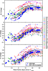 |
Fig. 6. Optical (B − V, V − r, V − i) broadband colors of LSQ13abf compared to those of the CSP-I SE SN sample corrected for Milky Way reddening (Stritzinger et al. 2018b). LSQ13abf is among the bluest objects and is consistent with the SN Ib intrinsic color-curve templates (dashed blue lines; Stritzinger et al. 2018a). This indicates LSQ13abf suffers minimal to no host-galaxy reddening. Note that objects are color-coded relative to spectroscopic sub-type as defined in the bottom-left panel of Fig. 5. |
5. Spectroscopy
The visual-wavelength spectra of LSQ13abf are plotted in Fig. 7 (top panel). To provide an aid to the visualization, over-plotted each raw spectrum (gray) is a smoothed version (colors). The main features characterizing the spectra include conspicuous He Iλλ5876, 6678, and 7065 features, which are clearly visible starting from the second spectrum taken a month post explosion. The first spectrum is largely devoid of features, and most resembles that of an SN Ic as indicated by the classification telegram (Morrell et al. 2013). Additional features in the second spectrum are attributed to the Ca II NIR triplet, O Iλ7774 and Fe II, with Fe IIλ5169 being the strongest Fe II feature and is marked in the figure. There is also a hint of a narrow Hα feature attributed to host-galaxy nebular emission.
 |
Fig. 7. Top: spectral sequence of LSQ13abf. Each visual-wavelength spectrum was scaled to an absolute flux level using the r-band photometry and are shown at rest wavelength. Reported next to each spectrum is its phase (rest-frame days from explosion epoch) and telescope used to make the observation. The zero-flux level for each spectrum is marked by a horizontal dashed line having the same color of the smoothed spectrum. The main spectral features at their rest wavelength are marked by vertical dashed lines and labeled. For the first spectrum, we report uncertain identifications with question marks and dashed lines pointing to the corresponding features. Bottom: NIR spectrum of LSQ13abf taken 36 days post explosion. Prominent spectral features and telluric regions are marked. The spectrum was absolute-flux calibrated using the coeval optical spectrum. |
The first spectrum exhibits a bluer continuum compared to subsequent ones. This is due to the rapid temperature evolution of the photosphere as the ejecta expand and cool over time. The deep absorption at about 6000 Å in the first spectrum could be due to Si IIλ6355 at ∼19 000 ± 500 km s−1, as is thought to be the case in other early SN Ic spectra (see Taubenberger et al. 2006, their Fig. 8). We label this identification with a question mark in the first spectrum in Fig. 7. In the second and third spectra, a feature appears present that could be associated with the same ion, Si II, but at lower velocity. We note that there could also be contribution from Na I D together with Si II, as seen in SN 2016coi (Prentice et al. 2018). However, Parrent et al. (2016) questioned the identification of Si IIλ6355 in early SE SN spectra and suggest that hydrogen could give rise to features between 6000 and 6400 Å. In our case this would imply a Hα velocity of about ∼27 700 ± 700 km s−1. We label this possible identification with another question mark in Fig. 7. There could be a tiny absorption feature related to Hβ at the same velocity of the alleged Hα feature that is also marked in the figure. This would resemble what was observed by Parrent et al. (2016, see their Fig. 2) for the Type Ic SN 1994I at −6 d from peak as well as in the Type Ib SN 2007Y (Stritzinger et al. 2009). The first spectrum also contains prevalent absorption features at 4200 Å and 4750 Å, which could be related to Fe II as in other SNe Ic (Taubenberger et al. 2006). The absorption at 4200 Å might also be related to other ions, like C III/N III (Modjaz et al. 2009). In SN 2016coi (Prentice et al. 2018), the feature at 4200 Å is attributed to a blend of Mg II, O II, and Fe II. The feature at 4750 Å in SN 2016coi is attributed to Fe II blended with Si II and Co II.
Our single NIR spectrum of LSQ13abf is plotted in the bottom panel of Fig. 7 with the location of the two strong telluric regions indicated with a telluric symbol. The continuum of the spectrum resembles that of a Rayleigh-Jeans black-body (BB) tail and contains a prevalent P Cygni He Iλ10830 feature, along with a weaker P Cygni feature corresponding to He Iλ20587. Features likely attributed to O Iλ9263 and O Iλ11287 are also present, while no discernible hydrogen features are detected.
In the top panel of Fig. 8, we compare the visual-wavelength spectra of LSQ13abf to those of three other well-observed SNe Ib with cooling tails post explosion. These include SN 1999ex (Hamuy et al. 2002), SN 2008D (from Modjaz et al. 2009) and iPTF13bvn (from Fremling et al. 2016) at a few days post explosion and a month later. There is a rather large variety of spectral features in the early “hot” spectra among these objects. iPTF13bvn shows clear He I features already at +2 d. SN 2008D has a spectrum that is basically a continuum with the exception of two clear features below 4500 Å, associated with He II and N III by Dessart et al. (2018) and with C III/N III and O III by Modjaz et al. (2009). These features are also observed in SLSNe (Quimby et al. 2007). LSQ13abf resembles a SN Ic, with Si II (or Hα) and two deep absorption features, possibly related to Fe II as in SNe Ic, dominating the continuum. The absorption at 4200 Å is, however, at the same position of the feature identified by Modjaz et al. (2009) and Dessart et al. (2018) for SN 2008D and visible in the top spectrum of Fig. 8. At later epochs, the spectra are almost identical, with similar He, Ca and O features, and therefore LSQ13abf matches a standard SN Ib. SN 1999ex has weak helium lines and was therefore referred to by Hamuy et al. (2002) as an SN Ib/c.
 |
Fig. 8. Top: visual-wavelength spectral comparison between LSQ13abf and the Type Ib SN 1999ex (Hamuy et al. 2002), SN 2008D (Modjaz et al. 2009), and iPTF13bvn (Fremling et al. 2016). Bottom: NIR spectral comparison between LSQ13abf, iPTF13bvn and SN 1999ex. |
A comparison of our NIR spectrum of LSQ13abf to NIR spectra of iPTF13bvn at +8.5 d and +79 d and a +31 d spectrum of SN 1999ex is provided in the bottom panel of Fig. 8. Overall the spectra are broadly similar with the He Iλ10830 line dominating the spectral region, though there are some differences in the strength and position of the minimum absorption of this feature.
We now present the line velocities of Fe IIλ5169 and He Iλ5876 as estimated from the position of maximum absorption of their P Cygni profile using the spectral analysis software misfits (Holmbo et al., in prep.). Plotted in Fig. 9 are the measured Fe IIλ5169 (left panel) and He Iλ5876 (right panel) velocities and these results are reported in Table 10. LSQ13abf has expansion velocities similar to the bulk of the CSP-I SE SN sample, which are also reported along with their power-law (PL) evolution in both panels. The inferred expansion velocities of LSQ13abf are used in concert with fitting other bolometric properties below to derive pertinent explosion parameters. We note that there is no clear detection of Fe IIλ5169 nor He Iλ5876 in the first spectrum and thus no velocity measurements.
 |
Fig. 9. Fe IIλ5169 (left) and He Iλ5876 (right) Doppler absorption velocities of LSQ13abf compared with values measured for objects in the CSP-I SE SN sample (Taddia et al. 2018b). |
Velocity of the spectral lines of LSQ13abf.
6. Bolometric light curve
Using our broadband optical photometry, we proceeded to construct spectral energy distributions (SEDs) for each epoch of observation. To do so, appropriate AB offsets from Table 16 of Krisciunas et al. (2017) were first added to the filtered photometry. Next reddening corrections were applied and the magnitudes were converted to monochromatic flux to construct SEDs, which were then each fit with a BB function. This provides a representation of the flux distribution, including also the wavelength regions not covered by our data. The resulting SEDs and best-fit BB functions are presented in the left-hand panel of Fig. 10. Inspection of the figure indicates that at the earliest epoch the BB functions peak around 3000 Å. As time evolves the BB peak progressively shifts towards longer wavelength as the photosphere cools. Cooling follows from the decrease in radioactive energy deposition combined with expansion of the ejecta. The corresponding BB temperature (TBB) is plotted in the right-center panel of Fig. 10. The early drop in temperature corresponds to the initial decreasing phase in the bluer optical light curves shown in Fig. 3. The value of TBB drops from 9300 K to 6100 K in the first 11 days. Subsequently, TBB remains nearly constant over a fortnight, and then again drops, reaching 4600 K by +50 d.
 |
Fig. 10. Left: spectral energy distributions (SEDs) of LSQ13abf based on Bgri photometry. The SEDs have been shifted by the addition of an arbitrary constant for clarity and phases relative to the explosion epoch are reported. The symbols for the filters are as in Fig. 3. Each SED is fit with a BB function (red solid line) providing estimates of (right, top) the total luminosity (LBB), (right, middle) the BB temperature (TBB), and (right, bottom) the BB radius (RBB). The early cooling phase is clearly visible with a prompt drop in the TBB. Right: top panel, LBB is fit with an Arnett model (solid red line), beginning from the fourth epoch post discovery when the process(es) producing the early peak is negligible. To perform the Arnett model fit, a peak velocity derived from the RBB at the time of Lmax (red dashed line in the bottom panel) was adopted. This BB velocity at peak was then reduced by ≈18%, which is the difference between the RBB and the photospheric radius (green dots) derived at later epochs from the Fe II velocity. The first two measurements of LBB, TBB, and RBB were also simultaneously fit with the post-shock breakout cooling model of Chevalier & Fransson (2008, blue line). The corresponding explosion parameters derived from the combined model are reported in the top-panel. Shown in magenta for comparison are the bolometric properties of a hydrodynamical model from Taddia et al. (2018b). |
By integrating the BB fits over wavelength from 0 to infinity and multiplying the result by 4 , where DL is the distance of the SN, we obtain the bolometric light curve of LSQ13abf plotted in the top-right panel of Fig. 10. The luminosity drops during the first 7 days of evolution, followed by a rise to peak value by +23 d. Upon reaching maximum the luminosity again drops, reaching the same luminosity of the early minimum (i.e., 1.3 ± 0.1 × 1042 erg s−1) after +50 d. LSQ13abf peaks at 2.6 ± 0.2 × 1042 erg s−1, while our measurement of its first early peak indicates a luminosity of ≈ 1.5 ± 0.1 × 1042 erg s−1. The errors on these luminosity measurements are dominated by the uncertainty on the distance.
The BB fits also provide a measure of the BB radius, RBB, which is plotted in the bottom-right panel of Fig. 10. RBB rapidly increases in the first 10 days, and then the rate-of-increase drops. Our BB-fits provide RBB values on the order of 1015 cm. We over plot the radii computed by multiplying the He I and Fe II velocities shown in Fig. 9 with their spectral phases from explosion time, which are respectively larger and smaller (∼18%) than the RBB. The Fe II velocity serves as a good proxy for the bulk-velocity of LSQ13abf’s ejecta to be used when modeling the bolometric properties (see also Branch et al. 2002; Richardson et al. 2006).
We also compare the bolometric light curve that we obtained through BB fits to that obtained with the SE SN bolometric corrections of Lyman et al. (2016), in particular we use their B- and V-band bolometric correction. The bolometric light curve obtained with the bolometric corrections is similarly shaped, but depending on the epoch it is as much as ∼20% fainter, probably due to the BB encompassing more UV flux than the assumed SEDs in Lyman et al. (2016).
7. Modeling
7.1. Early post shock-breakout cooling and Arnett model
Armed with the bolometric properties and the velocity measurements, we proceed to infer key explosion parameters of LSQ13abf. The main peak of the bolometric light curve is powered by the radioactive decay of 56Ni and can be reproduced by an Arnett (1982) model, which has the 56Ni mass, the ejecta mass (Mej) and the kinetic energy (EK) of the explosion as free parameters. In the model calculations a mean opacity κopt = 0.07 cm2 g−1 is adopted (but see Wheeler et al. 2015), a constant density is assumed for the ejecta, and we impose the condition that EK/Mej = 3/10  (see Wheeler et al. 2015), where vFe is the Fe IIλ5169 velocity at the epoch of bolometric peak. Since there are no vFe measurements at peak, but RFe is about 18% lower than the value associated with the RBB at later epochs (see the bottom-right panel of Fig. 10), we use the velocity from the RBB at bolometric peak to infer a value for vFe. This corresponds to a value of vFe = 7300 km s−1 reduced by 18%, which is vFe = 6000 km s−1.
The Arnett model is valid during the photospheric phase when radioactivity is powering the light curve and there is minimal γ-ray escape. At early epochs, when the first peak is observed and the temperature drops quickly, the SN emission is likely produced by another energy source. Therefore, we apply an alternative model at these early epochs. In the literature, the early-phase bolometric properties of SN 2008D were nicely reproduced by an analytic model describing the cooling of the ejecta after the shock breakout (SBO; Chevalier & Fransson 2008). Modjaz et al. (2009) show a good fit of this model to estimates of SN 2008D’s LBB, RBB and TBB. The post-SBO cooling of the ejecta is a promising mechanism to explain the early peak of LSQ13abf, given its similarity to SN 2008D, and we attempt to fit the same model to LSQ13abf. The Chevalier & Fransson (2008) model not only has Mej and EK as free parameters, but also the progenitor radius ( ).
).
A simultaneous fit of the Chevalier & Fransson (2008) model to LBB, RBB and TBB during the first two epochs and of the Arnett model to LBB during the photospheric phase (+4 d to +40 d) provides the 56Ni mass, EK, Mej,  , and the explosion epoch. The best fit is shown in the right panels of Fig. 10, where the Arnett model is plotted with a red line and the Chevalier & Fransson (2008) model is plotted with a blue line. The initial decline phase and the later rise to maximum light are approximately fit by this combined model. The best-fit explosion parameters from the combined model fit are: 56Ni content of 0.16 ± 0.01(0.02) M⊙, EK = [1.27 ± 0.04(0.23)] × 1051 ergs, Mej = 5.94 ± 0.14(1.09) M⊙, an explosion epoch of JD 2456395.80±0.20, and
  R⊙. The errors quoted outside the parentheses correspond to the fit uncertainties and those quoted between parentheses are obtained assuming a 18% uncertainty on the photospheric velocity, a further 7% error due to the uncertainty on the distance, and in the case of the 56Ni mass estimates, an additional 10% error to be conservative.
Khatami & Kasen (2019) recently provided an analytic model for determining the 56Ni mass in radioactively-powered SNe. Their Eq. (A.12) applied to LSQ13abf would indicate a larger 56Ni mass as compared to that from the Arnett model: 0.27 M⊙ vs. 0.16 M⊙, assuming β = 9/8).
The analytical work of Arnett (1982) is based on a number of underlying assumptions that may pose problems for the application to SE SNe and therefore we should take results from this approach with caution. For example, the Arnett scaling relations depend sensitively on the choice of velocity which does have a number of shortcoming (see Mazzali et al. 2013, for a discussion). Furthermore, there is also an inherent uncertainty when adopting a constant mean opacity as highlighted by more sophisticated hydrodynamical model results presented by Dessart et al. (2016, see their Fig. 19). A constant mean opacity cannot be tuned to match the light curves of models with variable opacity. However, we do stress that making use of both hydrodynamical and Arnett (1982) models to estimate explosion parameters of an extended sample of SE SNe does produce rather consistent results, as demonstrated in Fig. 24 of Taddia et al. (2018b). In the case of LSQ13abf, we note that a comparison between the constant-opacity Arnett model results and those obtained from a more sophisticated hydrodynamical model presented below, provide similar explosion parameters.
A constant opacity is also assumed in the Chevalier & Fransson (2008) model. Indeed, as the authors mention in their work, a requirement of the applicability of the model is a constant opacity, a condition that will break when the gas recombines to the ground state as the temperature drops. Dessart et al. (2011) and Piro & Nakar (2013) noticed that when the recombination temperature is reached the temperature and the luminosity of a SN remain constant resulting in a plateau-like evolution. This temperature should be around 7000 K (0.6 eV), which is reached by LSQ13abf only after the first two photometric epochs while it exhibits a period of cooling. This is why to compute the Chevalier & Fransson (2008) model fit to the data only the first two epochs of photometry are used when cooling is ongoing and the recombination temperature has not yet been reached.
7.2. Extended-envelope and Arnett model
We also attempt to reproduce the bolometric properties of LSQ13abf with the combination of an Arnett model for the main peak and the extended-envelope model for the early epochs as in Nakar & Piro (2014) and Piro (2015). The result, shown in Fig. 11, is worse than that using the model of Chevalier & Fransson (2008). This is not surprising as the early peak is observed in the bluer bands but not in the redder bands, and it was noticed by Nakar & Piro (2014) that this is more consistent with a regular structure of the progenitor star and not with the presence of an extended envelope. The best fit parameters (see Fig. 11) are similar to those obtained by fitting Chevalier & Fransson (2008), again with a progenitor radius of a few ×10 R⊙. In the case of the extended-envelope model the explosion epoch would be 2.6 days earlier than the one estimated by fitting the Chevalier & Fransson (2008) model.
 |
Fig. 11. As in Fig. 10, this time the early epochs are fit with a post-shock breakout extended-envelope model (Piro 2015), and the later epochs are simultaneously fit with an Arnett model. The best fit of this combined model provides a worse match to the early TBB and RBB profiles and to the main peak as compared to the combined Arnett + Chevalier & Fransson model. |
7.3. Companion Interaction and Arnett model
A better fit to the bolometric properties at early epochs is obtained by fitting the companion interaction model of Kasen (2010), for a binary separation of 143 R⊙. The best fit is shown in Fig. 12. Here we assume 45 deg for the viewing angle defined between the observer direction and the SN-companion interaction region. We note that the viewing angle can significantly impact the derived binary distance. For example, with a viewing angle of 45° we obtained 143 R⊙, but if 10 degrees is assumed, the distance increases to 2370 R⊙.
 |
Fig. 12. As in Fig. 10, this time the early epochs are fit with a companion shock-interaction model (Kasen 2010) and the later epochs are simultaneously fit with an Arnett model. The best-fit model reproduces all the observables of the first two epochs. The binary semi-major axis is given by a = 143 R⊙. |
Despite the fact that the Kasen (2010) model produces a good fit to the early light curve of LSQ13abf, population synthesis modeling presented by Moriya et al. (2015) indicated that the probability of the early light curve of SNe Ib/c is brightened due to collision is ≈0.56%.
7.4. Magnetar model
LSQ13abf shows a double peak in the light curves and this makes it different from more typical SNe Ib observed, for example, in the sample (see Fig. 5). However, LSQ13abf does not resemble extremely peculiar objects like SN 2005bf (Anupama et al. 2005; Tominaga et al. 2005; Folatelli et al. 2006; Maeda et al. 2007) or PTF11mnb (Taddia et al. 2018a), whose double-peaked light curves had a much longer timescale and for which a magnetar was invoked as one of the possible powering mechanisms. Therefore, in the case of LSQ13abf, there appears to be no evidence for invoking a magnetar model (Kasen & Bildsten 2010). Even if we assume that the early peak is powered by a magnetar as in Kasen et al. (2016), we cannot reproduce the luminosity and the time scale of the early peak given the values of EK and Mej from the previous models of the main peak, for standard values of the magnetic field intensity and the magnetar spin period.
7.5. Hydrodynamical models with a double 56Ni distribution
We identified a published hydrodynamical model that reproduces the main peak of the bolometric light curves, the temperature evolution, and the radius. This model was among those produced to fit the CSP-I SE SN sample (Taddia et al. 2018b) and was computed using a code developed by Bersten et al. (2011, 2013). The bolometric light curve of this model –named He8E3Ni15 – is plotted as magenta lines in Fig. 10. The model reproduces the observations after +10 d when radioactivity dominates the energy deposition and the progenitor radius does not have a significant impact on the shape of the light curve.
The He8E3Ni15 model is characterized by an Mej ≈ 6.2 M⊙, similar to our estimate from Arnett (Mej ≈ 5.94 ± 0.14 M⊙). The 56Ni mass is also similar: 0.15 M⊙ vs. 0.16 ± 0.02 M⊙, while the energy is larger in the hydrodynamical model: EK ≈ 3.0 × 1051 erg s−1 vs. 1.27 ± 0.04 × 1051 ergs. The hydrodynamical model reproduces the RBB and not the photospheric radius derived from the vFe which indicates the need for a larger EK. The progenitor star used to produce this hydrodynamical model was a He-rich star that evolved from a single star with a mass of 25 M⊙ (Taddia et al. 2018b).
Bersten et al. (2013) present two different scenarios for the bright early peak of SN 2008D. This includes a double 56Ni distribution and a progenitor structure with an extended envelope, that is a star with a dense compact core with a diffuse, extended low-mass envelope. In principle, both scenarios produce a brighter minimum between the early peak and the main peak, as observed in SN 2008D and LSQ13abf.
In Fig. 13, the bolometric light curve of LSQ13abf is compared with that of SN 2008D and the Bersten et al. (2013) double 56Ni distribution model. LSQ13abf appears more luminous than SN 2008D in the days and weeks following their explosion epochs. Within the context of a double 56Ni distribution, a model with both a larger 56Ni mass in the inner part and in the outer part and/or a more centralized inner 56Ni distribution would allow for a decent fit to the light curve.
 |
Fig. 13. Same as Fig. 5 from Bersten et al. (2013), adapted to show the comparison between the bolometric light curve of LSQ13abf (green line) to their double 56Ni-distribution model. The arrows show the effects of increasing the amount of 56Ni (i.e., M(56Ni)) in the outer distribution, the velocity of the inner distribution of 56Ni (i.e., v(56Ni)in), and the velocity of the outer distribution of 56Ni (i.e., v(56Ni)out). |
Dessart et al. (2018) notice that in the case of SN 2008D, the helium lines are rather narrow around peak. This is in conflict with the presence of 56Ni in the other ejecta as suggested by Bersten et al. (2013), which would produce broader helium features.
Comparing the spectra of LSQ13abf with those of SN 2008D and iPTF13bvn displayed in the top-panel of Fig. 8, reveals LSQ13abf also exhibits narrow helium features with standard expansion velocities (see Fig. 9). Given this, the double 56Ni distribution model is unlikely to provide a better explanation than the post-SBO cooling model.
A relatively low degree of 56Ni mixing is also suggested by the comparison of the early colors of LSQ13abf to the models developed by Yoon et al. (2019). We show this comparison in Fig. 14, where low degree of 56Ni mixing (fm) produce models with double-peaked color curves, while strong 56Ni mixing produces monotonically-rising color curves. LSQ13abf shows a double peak in the color curves, and a slow rise to the second main peak, like other SNe Ib in the literature, and in contrast to most SNe Ic, as shown by Yoon et al. (2019) in their Fig. 11.
 |
Fig. 14. (B − V) and (V − R) color-curve evolution of LSQ13abf compared to the synthetric color-curve evolution of five SN Ib models presented by Yoon et al. (2019) covering various degrees of 56Ni mixing (fm). The comparison suggests LSQ13abf experienced a low amount of 56Ni mixing, that is fm ∼ 0.15 − 0.3. |
7.6. Hydrodynamical models with an extended envelope
To facilitate a comparison with the findings of Bersten et al. (2013), in Fig. 15 the bolometric light curve of LSQ13abf is overlaid on their Fig. 9. The extended envelope models (blue thin lines) do reproduce a bright minimum as in the case of SN 2008D and are characterized by  . LSQ13abf would require a more extended radius due to its early phase light curve being more luminous, as well as a more extended structure to explain the luminosity of the early minimum.
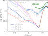 |
Fig. 15. Same as Fig. 9 from Bersten et al. (2013) adapted to show a comparison of the bolometric light curve of LSQ13abf (green line) to their extended envelope models. |
An example of a larger extended envelope is a SN Ib model presented by Dessart et al. (2018). Their model produces an early light curve for a He-giant progenitor star with an extended envelope of 173 R⊙, a relatively low ZAMS mass (12 M⊙), and a pre-SN mass of ∼2.73 M⊙. They account only for the early part of the SN light curve and do not consider the presence of radioactive 56Ni. The extended envelope consists of 0.074 M⊙, Mej ∼ 1 M⊙, and EK ∼ 1 × 1051 ergs. Their model overestimates the early luminosity of SN 2008D, however as demonstrated in the top panel of Fig. 16, the synthetic absolute BVRI-band light curves match reasonably well the first two epochs of the light curves of LSQ13abf.
 |
Fig. 16. Top: early light curve comparison to the model of the explosion of a He-giant star with extended envelope (173 R⊙) from Dessart et al. (2018). Bottom: comparison of early spectra of the Type Ib SN 2008D, iPTF13bvn and LSQ13abf with synthetic spectra. |
The Dessart et al. (2018) model has not been fine-tuned to match the main peak of LSQ13abf, as it lacks 56Ni, and more importantly, the Mej is too low and therefore would result in a narrower light curve than what is observed. The EK is similar to our estimate, that is 1.0 × 1051 ergs vs. 1.3 × 1051 ergs from our Arnett model. A different value of EK/Mej would affect the value for the R* if the model is fit to the early emission. A higher EK/Mej ratio pushes R* to higher values, assuming the formulas for the extended envelope radius in Nakar & Piro (2014). Scaling R* in the Dessart et al. (2018) model using the Nakar & Piro (2014) expression and the values of EK and Mej from our Arnett model, we obtain an extended envelope radius of 226 R⊙ for LSQ13abf. Assuming EK and Mej from the hydrodynamical model shown in Fig. 10 (magenta lines), then the envelope R* would be 108 R⊙. In any case, the radius of the extended envelope of LSQ13abf would be larger than that of SN 2008D, that is  . In the bottom panel of Fig. 16, the synthetic spectra from the extended-envelope model computed by Dessart et al. (2018) are compared with the early spectra shown in the top panel of Fig. 8, including the first spectrum of LSQ13abf and early spectra of SN 2008D and iPTF13bvn. The synthetic spectra exhibit He I lines as soon as He IIλ4686 vanishes (after +2 d). There are no discernible helium features in LSQ13abf at this phase. The absorption minimum located in LSQ13abf around 6000 Å is likely related to Si II (or Hα) and is not present in the model spectra, as well as the strong features at 4400 Å and 4750 Å, which might be attributed to Fe II features. Our spectrum is not as early as the first SN 2008D spectrum which according to Dessart et al. (2018) shows He II and N III around 4000–4300 Å. Note however, Modjaz et al. (2009) attributes these features to C III and O III, respectively.
Despite the differences, the synthetic spectra of Dessart et al. (2018) for their extended envelope model have diluted features and the He I features take time to emerge, just as seen in LSQ13abf. A spectral model by Dessart et al. (2018, see their Fig. 8) for a similar progenitor, but without the extended envelope, shows prominent He I features at early epochs and a non-diluted spectrum.
8. Discussion
8.1. Model parameters of the early SN Ib sample
How do these explosion parameters compare to those of the progenitors of our small comparison sample of SNe Ib with documentation of an early peak? To answer this question we apply the combined Chevalier & Fransson (2008) and Arnett (1982) model to the bolometric properties of SN 1999ex, SN 2008D and iPTF13bvn as obtained from Stritzinger et al. (2002), Modjaz et al. (2009) and Fremling et al. (2016), respectively. The model fits to the early peak and the photospheric phase LBB, TBB, and RBB profiles of SN 1999ex, SN 2008D, iPTF13bvn, and LSQ13abf are shown in Fig. 17 and the best-fit model parameters are summarized in Table 11. To compute these fits it was assumed that the BB velocity tracks the photospheric velocity, since the BB velocity and vFe were found to be very similar for iPTF13bvn (Fremling et al. 2014). Inspection of Fig. 17 reveals that the post-SBO cooling model reproduces the bolometric properties during the post-SBO cooling phase and the photospheric phase for each of the comparison objects.
 |
Fig. 17. Bolometric properties of SNe 1999ex, 2008D, iPTF13bvn, and LSQ13abf reproduced by the combined Arnett and Chevalier & Fransson model discussed in Sect. 7. The derived progenitor radii are reported in the top panel. |
With values of  R⊙,
R⊙,  R⊙ and
  R⊙, the Chevalier & Fransson (2008) model suggests their progenitors are more compact as compared to that of LSQ13abf with an inferred value of
  R⊙. Interestingly, with a combined model fit providing
  M⊙, LSQ13abf also appears to originate from a more massive progenitor relative to not only our comparison sample with early peak, but also relative to average values (≲4 M⊙) inferred from various SN Ib sample studies (see Fig. 25 in Taddia et al. 2018b). These findings are consistent with LSQ13abf being both significantly brighter than the comparison sample during the post-SBO phase and exhibiting a broader light curve during its rise and decline to and from maximum.
8.2. LSQ13abf progenitor scenario
As previously mentioned, the majority of SE SNe likely originate from relatively low-mass progenitors, well below the canonical mass (i.e., ZAMS mass ∼25 M⊙) where it is possible for solitary massive stars to shed their hydrogen envelopes via steady-state line-driven winds over their evolutionary lifetimes4. Therefore, many of the progenitors of SE SNe are thought to be in interacting binaries that shed their hydrogen envelopes through Roche-lobe overflow to a companion. Both the Arnett and hydrodynamical models of LSQ13abf suggest a large ejecta mass for a SN Ib (5.9−6.2 M⊙), which is compatible with a ZAMS mass of ∼25 M⊙. This suggests that LSQ13abf is among the more massive SN Ib yet studied. Contrary to most other SE SNe that have less-massive progenitors and are likely in an interacting binary systems, the high-mass inferred for LSQ13abf may imply it is associated with a single star. However, we note that massive stars can also be members of binary star systems (see, e.g., Yoon 2015). In short, it is difficult for us to ascertain if its origins lie in a single or binary progenitor.
A comparison of the early observations of LSQ13abf to the hydrodynamical models of Bersten et al. (2013) and Dessart et al. (2018), also suggests the presence of an extended envelope (i.e., R* ∼ 100 R⊙). However, these models are not entirely consistent with LSQ13abf as we not only favor a He-star progenitor with an extended envelope, but as mentioned above, a progenitor more massive than considered in these models and others in the literature.
Hydrogen-rich single massive stars close to the Eddington limit can also produce inflated envelopes (Ishii et al. 1999; Petrovic et al. 2006; Sanyal et al. 2015; Fuller 2017), although their R* are generally predicted to be smaller than those of relatively low mass He-giant stars in binary systems. In principle, similar to the H-rich scenario, solitary massive He stars near the Eddington limit could also suffer significant envelope inflation (Gräfener et al. 2012). To our knowledge there are no observations or models in the literature of massive (> 25 M⊙) He stars with significantly extended envelopes. However, Fuller & Ro (2018) presented a simulation of a 5 M⊙ He-star evolved from a 15 M⊙ ZAMS star, stripped of hydrogen through companion interaction, and during its pre-SN evolution significantly inflates its envelope via a super-Eddington wind driven by energy thermalized in the outer layers that ultimately originates from deep within the core of the star and transferred by internal gravity waves (Quataert & Shiode 2012). Along these lines, we suggest that the progenitor of LSQ13abf might have been a single or a binary, massive He-star with a significantly inflated envelope. Although beyond the scope of this paper, we do encourage others in the community to further investigate such progenitors.
In the case of SN 2008D, Soderberg et al. (2008) favored a massive WR progenitor star, while Modjaz et al. (2009) concluded  would be consistent with the typical radius of a massive WN star. However, Dessart et al. (2018) argued that the progenitor was a low-mass He-giant star in a binary system. While a low-mass He-giant star in a binary system would naturally produce the significant emission observed at early epochs of SN 2008D and LSQ13abf, it is not consistent with the high ejecta mass we obtained for both objects (see Table 11).
Regardless of the binary or single nature of the progenitor system, we find the radius of the precursor was larger than that of the other SNe Ib with published observations documenting an early peak. In a post-SBO cooling scenario with a regular progenitor structure, as modeled using Chevalier & Fransson (2008), LSQ13abf’s progenitor star at the moment of explosion had  . This is three times
  assuming the same model. If we consider the extended-envelope structure, as suggested by the hydrodynamical models in Bersten et al. (2013) and Dessart et al. (2018), then
  might be even larger compared to that of SN 2008D, perhaps on the order of
  .
.
9. Conclusion
We present early photometry and spectroscopy of the SN Ib LSQ13abf, which shows an early peak in the bluer bands as in a few other cases in the literature. Based on both semi-analytical and hydrodynamical models from the literature, we find that the progenitor star of LSQ13abf had a larger radius than those of SNe Ib including SN 1999ex, SN 2008D and iPTF13bvn, all of which were observed during the post-SBO cooling phase. Hydrodynamical models of He stars in interacting binaries suggests a progenitor structure with an extended envelope attached to a dense core. The high Mej estimate points toward LSQ13abf originating from a massive pre-SN progenitor that likely evolved from a MZAMS ≳ 25 M⊙ star. Such a progenitor could be in a binary or single star system. No matter the exact nature of the progenitor, modern simulations of high mass stars do not exhibit extended envelopes as inferred for LSQ13abf. We therefore hope that this study provides impetus for others to further explore scenarios of single, massive He-stars with inflated envelopes that might ultimately produce objects similar to LSQ13abf.
In Sect. 7, we estimate the explosion epoch to have occurred on JD 2456395.80±0.20. This value is used to compute the phase of our SN observations.
Depending on adopted mass-loss models as well as stellar metalicity and rotation, the minimum ZAMS mass required for single stars to drive robust enough line-driven winds to strip the hydrogen envelope could be as much as 40 M⊙ (see, e.g., Smith et al. 2011, for a discussion and references therein).
Acknowledgments
A special thank you to the referee for their constructive report. We thank Takashi Jose Moriya, Thomas Tauris, and Paolo Mazzali for fruitful discussions. We acknowledge Jeffrey Silverman for reducing the HET spectroscopic observations, and Peter Nugent and David Rabinowitz for providing LSQ images. M.S., F.T., and E.K. are funded by a project grant (8021-00170B) from the Independent Research Fund Denmark. M.S. and S.H. are supported in part by a generous grant (13261) from VILLUM FONDEN. E.B. acknowledges support from NASA Grant: NNX16AB25G. N.B.S. acknowledges support from the NSF through grant AST-1613455, and through the Texas A&M University Mitchell/Heep/Munnerlyn Chair in Observational Astronomy. L.G. is supported by the European Union’s Horizon 2020 research and innovation programme under the Marie Skłodowska-Curie grant agreement No. 839090. The CSP-II has been funded by the USA’s NSF under grants AST-0306969, AST-0607438, AST-1008343, AST-1613426, AST-1613455, and AST-1613472, and in part by a Sapere Aude Level 2 grant funded by the Danish Agency for Science and Technology and Innovation (PI M.S.). The research of JCW is supported in part by NSF AST-1813825. This work is partly based on observations made with the Nordic Optical Telescope, operated by the Nordic Optical Telescope Scientific Association at the Observatorio del Roque de los Muchachos, La Palma, Spain, of the Instituto de Astrofisica de Canarias. Visual-wavelength spectra of LSQ13abf were obtained in part with ALFOSC, which is provided by the Instituto de Astrofisica de Andalucia (IAA) under a joint agreement with the University of Copenhagen and NOTSA.
References
- Albareti, F. D., Allende Prieto, C., Almeida, A., et al. 2017, ApJS, 233, 25 [NASA ADS] [CrossRef] [Google Scholar]
- Anupama, G. C., Sahu, D. K., Deng, J., et al. 2005, ApJ, 631, L125 [NASA ADS] [CrossRef] [Google Scholar]
- Arcavi, I., Gal-Yam, A., Yaron, O., et al. 2011, ApJ, 742, L18 [NASA ADS] [CrossRef] [Google Scholar]
- Arnett, W. D. 1982, ApJ, 253, 785 [NASA ADS] [CrossRef] [Google Scholar]
- Bianco, F. B., Modjaz, M., Hicken, M., et al. 2014, ApJS, 213, 19 [NASA ADS] [CrossRef] [Google Scholar]
- Becker, A. 2015, Astrophysics Source Code Library [record ascl:1504.004] [Google Scholar]
- Bersten, M. C., Benvenuto, O., & Hamuy, M. 2011, ApJ, 729, 61 [NASA ADS] [CrossRef] [Google Scholar]
- Bersten, M. C., Tanaka, M., Tominaga, N., Benvenuto, O. G., & Nomoto, K. 2013, ApJ, 767, 143 [NASA ADS] [CrossRef] [Google Scholar]
- Branch, D., Benetti, S., Kasen, D., et al. 2002, ApJ, 566, 1005 [NASA ADS] [CrossRef] [Google Scholar]
- Brown, P. J., Holland, S. T., Immler, S., et al. 2009, AJ, 137, 4517 [NASA ADS] [CrossRef] [Google Scholar]
- Cano, Z., Bersier, D., Guidorzi, C., et al. 2011, ApJ, 740, 41 [NASA ADS] [CrossRef] [Google Scholar]
- Chevalier, R. A. 1992, ApJ, 394, 599 [NASA ADS] [CrossRef] [Google Scholar]
- Chevalier, R. A., & Fransson, C. 2008, ApJ, 683, L135 [NASA ADS] [CrossRef] [Google Scholar]
- Clocchiatti, A., Wheeler, J. C., & Barker, E. S. 1995, ApJ, 446, 167 [NASA ADS] [CrossRef] [Google Scholar]
- Contreras, C., Phillips, M. M., Burns, C. R., et al. 2018, AJ, 859, 24 [NASA ADS] [CrossRef] [Google Scholar]
- De, K., Kasliwal, M. M., Ofek, E. O., et al. 2018, Science, 362, 201 [NASA ADS] [CrossRef] [Google Scholar]
- D’Elia, V., Pian, E., Melandri, A., et al. 2015, A&A, 577, A116 [NASA ADS] [CrossRef] [EDP Sciences] [Google Scholar]
- Dessart, L., Hillier, D. J., Livne, E., et al. 2011, MNRAS, 414, 2985 [NASA ADS] [CrossRef] [Google Scholar]
- Dessart, L., Hillier, D. J., Woosley, S., et al. 2016, MNRAS, 458, 1618 [NASA ADS] [CrossRef] [Google Scholar]
- Dessart, L., Yoon, S.-C., Livne, E., et al. 2018, A&A, 612, A61 [NASA ADS] [CrossRef] [EDP Sciences] [Google Scholar]
- Drout, M. R., Milisavljevic, D., Parrent, J., et al. 2016, ApJ, 821, 57 [NASA ADS] [CrossRef] [Google Scholar]
- Fitzpatrick, E. L. 1999, PASP, 111, 63 [NASA ADS] [CrossRef] [Google Scholar]
- Folatelli, G., Contreras, C., Phillips, M. M., et al. 2006, ApJ, 641, 1039 [NASA ADS] [CrossRef] [Google Scholar]
- Fremling, C., Sollerman, J., Taddia, F., et al. 2014, A&A, 565, A114 [NASA ADS] [CrossRef] [EDP Sciences] [Google Scholar]
- Fremling, C., Sollerman, J., Taddia, F., et al. 2016, A&A, 593, A68 [NASA ADS] [CrossRef] [EDP Sciences] [Google Scholar]
- Fremling, C., Ko, H., Dugas, A., et al. 2019, ApJ, 878, L5 [NASA ADS] [CrossRef] [Google Scholar]
- Fuller, J. 2017, MNRAS, 470, 1642 [NASA ADS] [CrossRef] [Google Scholar]
- Fuller, J., & Ro, S. 2018, MNRAS, 476, 1853 [NASA ADS] [CrossRef] [Google Scholar]
- Galbany, L., Anderson, J. P., Sánchez, S. F., et al. 2018, ApJ, 855, 107 [NASA ADS] [CrossRef] [Google Scholar]
- Gräfener, G., Owocki, S. P., & Vink, J. S. 2012, A&A, 538, A40 [NASA ADS] [CrossRef] [EDP Sciences] [Google Scholar]
- Habets, G. M. H. J. 1986a, A&A, 165, 95 [NASA ADS] [Google Scholar]
- Habets, G. M. H. J. 1986b, A&A, 167, 61 [NASA ADS] [Google Scholar]
- Hadjiyska, E., Rabinowitz, D., Baltay, C., et al. 2012, New Horiz. Time Domain Astron., 285, 324 [NASA ADS] [Google Scholar]
- Hamuy, M., Suntzeff, N. B., Gonzalez, R., & Martin, G. 1988, AJ, 95, 63 [NASA ADS] [CrossRef] [Google Scholar]
- Hamuy, M., Maza, J., Pinto, P. A., et al. 2002, AJ, 124, 417 [NASA ADS] [CrossRef] [Google Scholar]
- Hamuy, M., Folatelli, G., Morrell, N., et al. 2006, PASP, 118, 2 [NASA ADS] [CrossRef] [Google Scholar]
- Hsiao, E. Y., Phiilips, M. M., Marion, G. H., et al. 2019, PASP, 131, 4002 [Google Scholar]
- Ishii, M., Ueno, M., & Kato, M. 1999, PASJ, 51, 417 [NASA ADS] [Google Scholar]
- Jerkstrand, A. 2017, Handbook of Supernovae, 795 [CrossRef] [Google Scholar]
- Kasen, D. 2010, ApJ, 708, 1025 [NASA ADS] [CrossRef] [Google Scholar]
- Kasen, D., & Bildsten, L. 2010, ApJ, 717, 245 [NASA ADS] [CrossRef] [Google Scholar]
- Kasen, D., Metzger, B. D., & Bildsten, L. 2016, ApJ, 821, 36 [NASA ADS] [CrossRef] [Google Scholar]
- Khatami, D. K., & Kasen, D. N. 2019, ApJ, 878, 56 [NASA ADS] [CrossRef] [Google Scholar]
- Krisciunas, K., Contreras, C., Burns, C. R., et al. 2017, AJ, 154, 211 [NASA ADS] [CrossRef] [Google Scholar]
- Komatsu, E., Dunkley, J., Nolta, M. R., et al. 2009, ApJS, 180, 330 [NASA ADS] [CrossRef] [Google Scholar]
- Landolt, A. U. 1992, AJ, 104, 372 [NASA ADS] [CrossRef] [Google Scholar]
- Leloudas, G., Chatzopoulos, E., Dilday, B., et al. 2012, A&A, 541, A129 [NASA ADS] [CrossRef] [EDP Sciences] [Google Scholar]
- Lyman, J. D., Bersier, D., James, P. A., et al. 2016, MNRAS, 457, 328 [NASA ADS] [CrossRef] [Google Scholar]
- Maeda, K., Tanaka, M., Nomoto, K., et al. 2007, ApJ, 666, 1069 [NASA ADS] [CrossRef] [Google Scholar]
- Malesani, D., Fynbo, J. P. U., Hjorth, J., et al. 2009, ApJ, 692, L84 [NASA ADS] [CrossRef] [Google Scholar]
- Mazzali, P. A., Valenti, S., Della Valle, M., et al. 2008, Science, 321, 1185 [NASA ADS] [CrossRef] [PubMed] [Google Scholar]
- Mazzali, P. A., Walker, E. S., Pian, E., et al. 2013, MNRAS, 432, 2463 [NASA ADS] [CrossRef] [Google Scholar]
- Mazzali, P. A., Sauer, D., Pian, E., et al. 2017, MNRAS, 469, 2498 [NASA ADS] [CrossRef] [Google Scholar]
- McClelland, L. A. S., & Eldridge, J. J. 2016, MNRAS, 459, 1505 [NASA ADS] [CrossRef] [Google Scholar]
- Modjaz, M., Li, W., Butler, N., et al. 2009, ApJ, 702, 226 [NASA ADS] [CrossRef] [Google Scholar]
- Morales-Garoffolo, A., Elias-Rosa, N., Benetti, S., et al. 2014, MNRAS, 445, 1647 [NASA ADS] [CrossRef] [Google Scholar]
- Morales-Garoffolo, A., Elias-Rosa, N., Bersten, M., et al. 2015, MNRAS, 454, 95 [NASA ADS] [CrossRef] [Google Scholar]
- Moriya, T. J., Liu, Z.-W., & Izzard, R. G. 2015, MNRAS, 450, 3264 [NASA ADS] [CrossRef] [Google Scholar]
- Morrell, N., Hsiao, E. Y., Stritzinger, M., et al. 2013, ATel, 4990 [Google Scholar]
- Nakar, E., & Piro, A. L. 2014, ApJ, 788, 193 [NASA ADS] [CrossRef] [Google Scholar]
- Nicholl, M., & Smartt, S. J. 2016, MNRAS, 457, L79 [NASA ADS] [CrossRef] [Google Scholar]
- Noebauer, U. M., Kromer, M., Taubenberger, S., et al. 2017, MNRAS, 472, 2787 [NASA ADS] [CrossRef] [Google Scholar]
- Parrent, J. T., Milisavljevic, D., Soderberg, A. M., et al. 2016, ApJ, 820, 75 [NASA ADS] [CrossRef] [Google Scholar]
- Persson, S. E., Murphy, D. C., Krzeminski, W., Roth, M., & Rieke, M. J. 1998, AJ, 116, 2475 [NASA ADS] [CrossRef] [Google Scholar]
- Petrovic, J., Pols, O., & Langer, N. 2006, A&A, 450, 219 [NASA ADS] [CrossRef] [EDP Sciences] [Google Scholar]
- Pettini, M., & Pagel, B. E. J. 2004, MNRAS, 348, L59 [NASA ADS] [CrossRef] [Google Scholar]
- Phillips, M. M., Contreras, C., Hsiao, E. Y., et al. 2019, PASP, 131, 4001 [Google Scholar]
- Pilyugin, L. S., Vílchez, J. M., & Contini, T. 2004, A&A, 425, 849 [NASA ADS] [CrossRef] [EDP Sciences] [Google Scholar]
- Piro, A. L. 2015, ApJ, 808, L51 [NASA ADS] [CrossRef] [Google Scholar]
- Prentice, S. J., Ashall, C., Mazzali, P. A., et al. 2018, MNRAS, 478, 4162 [NASA ADS] [CrossRef] [Google Scholar]
- Prentice, S. J., Ashall, C., James, P. A., et al. 2019, MNRAS, 485, 1559 [NASA ADS] [CrossRef] [Google Scholar]
- Piro, A. L., & Nakar, E. 2013, ApJ, 769, 67 [NASA ADS] [CrossRef] [Google Scholar]
- Quataert, E., & Shiode, J. 2012, MNRAS, 423, L92 [NASA ADS] [CrossRef] [Google Scholar]
- Quimby, R. M., Aldering, G., Wheeler, J. C., et al. 2007, ApJ, 668, L99 [NASA ADS] [CrossRef] [Google Scholar]
- Rabinak, I., & Waxman, E. 2011, ApJ, 728, 63 [NASA ADS] [CrossRef] [Google Scholar]
- Richardson, D., Branch, D., & Baron, E. 2006, AJ, 131, 2233 [NASA ADS] [CrossRef] [Google Scholar]
- Richmond, M. W., Treffers, R. R., Filippenko, A. V., et al. 1994, AJ, 107, 1022 [NASA ADS] [CrossRef] [Google Scholar]
- Sanyal, D., Grassitelli, L., Langer, N., & Bestenlehner, J. M. 2015, A&A, 580, A20 [NASA ADS] [CrossRef] [EDP Sciences] [Google Scholar]
- Schlafly, E. F., & Finkbeiner, D. P. 2011, ApJ, 737, 103 [NASA ADS] [CrossRef] [Google Scholar]
- Simcoe, R. A., Burgasser, A. J., Schechter, P. L., et al. 2013, PASP, 125, 270 [NASA ADS] [CrossRef] [Google Scholar]
- Smartt, S. J. 2015, PASA, 32, e016 [NASA ADS] [CrossRef] [Google Scholar]
- Smith, J. A., Tucker, D. L., Kent, S., et al. 2002, AJ, 123, 2121 [Google Scholar]
- Smith, N., Li, W., Filippenko, A. V., et al. 2011, MNRAS, 412, 1522 [NASA ADS] [CrossRef] [Google Scholar]
- Soderberg, A. M., Berger, E., Page, K. L., et al. 2008, Nature, 453, 469 [NASA ADS] [CrossRef] [PubMed] [Google Scholar]
- Sollerman, J., Jaunsen, A. O., Fynbo, J. P. U., et al. 2006, A&A, 454, 503 [NASA ADS] [CrossRef] [EDP Sciences] [Google Scholar]
- Stritzinger, M., Hamuy, M., Suntzeff, N. B., et al. 2002, AJ, 124, 2100 [NASA ADS] [CrossRef] [Google Scholar]
- Stritzinger, M. D., Mazzali, P. A., & Phillips, M. M. 2009, ApJ, 696, 713 [NASA ADS] [CrossRef] [Google Scholar]
- Stritzinger, M. D., Taddia, F., Burns, C. R., et al. 2018a, A&A, 609, A135 [NASA ADS] [CrossRef] [EDP Sciences] [Google Scholar]
- Stritzinger, M. D., Anderson, J. P., Contreras, C., et al. 2018b, A&A, 609, A134 [NASA ADS] [CrossRef] [EDP Sciences] [Google Scholar]
- Taddia, F., Sollerman, J., Razza, A., et al. 2013, A&A, 558, A143 [NASA ADS] [CrossRef] [EDP Sciences] [Google Scholar]
- Taddia, F., Sollerman, J., Fremling, C., et al. 2015a, A&A, 580, A131 [NASA ADS] [CrossRef] [EDP Sciences] [Google Scholar]
- Taddia, F., Sollerman, J., Leloudas, G., et al. 2015b, A&A, 574, A60 [NASA ADS] [CrossRef] [EDP Sciences] [Google Scholar]
- Taddia, F., Fremling, C., Sollerman, J., et al. 2016, A&A, 592, A89 [NASA ADS] [CrossRef] [EDP Sciences] [Google Scholar]
- Taddia, F., Sollerman, J., Fremling, C., et al. 2018a, A&A, 609, A106 [NASA ADS] [CrossRef] [EDP Sciences] [Google Scholar]
- Taddia, F., Stritzinger, M. D., Bersten, M., et al. 2018b, A&A, 609, A136 [NASA ADS] [CrossRef] [EDP Sciences] [Google Scholar]
- Taubenberger, S., Pastorello, A., Mazzali, P. A., et al. 2006, MNRAS, 371, 1459 [NASA ADS] [CrossRef] [Google Scholar]
- Tominaga, N., Tanaka, M., Nomoto, K., et al. 2005, ApJ, 633, L97 [NASA ADS] [CrossRef] [Google Scholar]
- Walker, E. S., Baltay, C., Campillay, A., et al. 2015, ApJS, 219, 13 [NASA ADS] [CrossRef] [Google Scholar]
- Wheeler, J. C., Johnson, V., & Clocchiatti, A. 2015, MNRAS, 450, 1295 [NASA ADS] [CrossRef] [Google Scholar]
- Xiang, D., Wang, X., Mo, J., et al. 2019, ApJ, 871, 176 [NASA ADS] [CrossRef] [Google Scholar]
- Yoon, S.-C. 2015, PASA, 32, 15 [NASA ADS] [CrossRef] [Google Scholar]
- Yoon, S.-C., Chun, W., Tolstov, A., et al. 2019, ApJ, 872, 174 [NASA ADS] [CrossRef] [Google Scholar]
All Tables
Optical photometry of the local sequence used in relation with LSQ imaging of LSQ13abf.
All Figures
|
Fig. 1. Finding chart of LSQ13abf constructed using a single r-band image obtained with the Swope 1 m telescope when the supernova was at peak brightness. The position of the SN (dotted circle) is shown within the inset in the upper right corner of the figure, and the optical (yellow circles) and NIR (red circles) local sequences are indicated. |
| In the text | |
|
Fig. 2. Host-galaxy spectrum of LSQ13abf. We indicate the main emission lines, which were fit with Gaussian functions (red) to measure the host-galaxy metalicity. The spectrum was corrected for MW extinction. The line fluxes are reported in Table 8. |
| In the text | |
|
Fig. 3. Absolute-magnitude light curves of LSQ13abf. Each light curve has been shifted by different amounts in magnitude (reported next to the name of each filter) for visual clarity. The optical light curves were fit with a low-order polynomial marked by dashed, thick lines of the same color of each light curve. The BVri light curves peak at +21.3, +21.1, +23.6, +27.6 d, respectively. The optical(NIR) spectral epochs are marked by black(red) segments at the bottom of the figure. We also report the corresponding absolute magnitudes of SN 2008D (Malesani et al. 2009) as solid colored lines, shifted by the same amounts used for LSQ13abf. The two SNe are remarkably similar when put into context with the light curve diversity among SE SN as shown in Fig. 5 of this paper. |
| In the text | |
|
Fig. 4. Comparison of the early absolute B-band light curve of LSQ13abf to the early U, b, B, g and r light curves of other SE SNe (one per sub-type), and for completeness the hydrogent dificient (Type I) SLSN 2006oz (Leloudas et al. 2012), which also exhibits a double peak. In the legend we report the filter and the SN type for each SN included in the comparison. |
| In the text | |
|
Fig. 5. Absolute magnitude, BVri-band light curves of LSQ13abf compared to those of the CSP-I SE SN sample (Stritzinger et al. 2018b; Taddia et al. 2018b). Objects are color-coded relative to spectroscopic sub-type as indicated in the bottom-left panel. |
| In the text | |
|
Fig. 6. Optical (B − V, V − r, V − i) broadband colors of LSQ13abf compared to those of the CSP-I SE SN sample corrected for Milky Way reddening (Stritzinger et al. 2018b). LSQ13abf is among the bluest objects and is consistent with the SN Ib intrinsic color-curve templates (dashed blue lines; Stritzinger et al. 2018a). This indicates LSQ13abf suffers minimal to no host-galaxy reddening. Note that objects are color-coded relative to spectroscopic sub-type as defined in the bottom-left panel of Fig. 5. |
| In the text | |
|
Fig. 7. Top: spectral sequence of LSQ13abf. Each visual-wavelength spectrum was scaled to an absolute flux level using the r-band photometry and are shown at rest wavelength. Reported next to each spectrum is its phase (rest-frame days from explosion epoch) and telescope used to make the observation. The zero-flux level for each spectrum is marked by a horizontal dashed line having the same color of the smoothed spectrum. The main spectral features at their rest wavelength are marked by vertical dashed lines and labeled. For the first spectrum, we report uncertain identifications with question marks and dashed lines pointing to the corresponding features. Bottom: NIR spectrum of LSQ13abf taken 36 days post explosion. Prominent spectral features and telluric regions are marked. The spectrum was absolute-flux calibrated using the coeval optical spectrum. |
| In the text | |
|
Fig. 8. Top: visual-wavelength spectral comparison between LSQ13abf and the Type Ib SN 1999ex (Hamuy et al. 2002), SN 2008D (Modjaz et al. 2009), and iPTF13bvn (Fremling et al. 2016). Bottom: NIR spectral comparison between LSQ13abf, iPTF13bvn and SN 1999ex. |
| In the text | |
|
Fig. 9. Fe IIλ5169 (left) and He Iλ5876 (right) Doppler absorption velocities of LSQ13abf compared with values measured for objects in the CSP-I SE SN sample (Taddia et al. 2018b). |
| In the text | |
|
Fig. 10. Left: spectral energy distributions (SEDs) of LSQ13abf based on Bgri photometry. The SEDs have been shifted by the addition of an arbitrary constant for clarity and phases relative to the explosion epoch are reported. The symbols for the filters are as in Fig. 3. Each SED is fit with a BB function (red solid line) providing estimates of (right, top) the total luminosity (LBB), (right, middle) the BB temperature (TBB), and (right, bottom) the BB radius (RBB). The early cooling phase is clearly visible with a prompt drop in the TBB. Right: top panel, LBB is fit with an Arnett model (solid red line), beginning from the fourth epoch post discovery when the process(es) producing the early peak is negligible. To perform the Arnett model fit, a peak velocity derived from the RBB at the time of Lmax (red dashed line in the bottom panel) was adopted. This BB velocity at peak was then reduced by ≈18%, which is the difference between the RBB and the photospheric radius (green dots) derived at later epochs from the Fe II velocity. The first two measurements of LBB, TBB, and RBB were also simultaneously fit with the post-shock breakout cooling model of Chevalier & Fransson (2008, blue line). The corresponding explosion parameters derived from the combined model are reported in the top-panel. Shown in magenta for comparison are the bolometric properties of a hydrodynamical model from Taddia et al. (2018b). |
| In the text | |
|
Fig. 11. As in Fig. 10, this time the early epochs are fit with a post-shock breakout extended-envelope model (Piro 2015), and the later epochs are simultaneously fit with an Arnett model. The best fit of this combined model provides a worse match to the early TBB and RBB profiles and to the main peak as compared to the combined Arnett + Chevalier & Fransson model. |
| In the text | |
|
Fig. 12. As in Fig. 10, this time the early epochs are fit with a companion shock-interaction model (Kasen 2010) and the later epochs are simultaneously fit with an Arnett model. The best-fit model reproduces all the observables of the first two epochs. The binary semi-major axis is given by a = 143 R⊙. |
| In the text | |
|
Fig. 13. Same as Fig. 5 from Bersten et al. (2013), adapted to show the comparison between the bolometric light curve of LSQ13abf (green line) to their double 56Ni-distribution model. The arrows show the effects of increasing the amount of 56Ni (i.e., M(56Ni)) in the outer distribution, the velocity of the inner distribution of 56Ni (i.e., v(56Ni)in), and the velocity of the outer distribution of 56Ni (i.e., v(56Ni)out). |
| In the text | |
|
Fig. 14. (B − V) and (V − R) color-curve evolution of LSQ13abf compared to the synthetric color-curve evolution of five SN Ib models presented by Yoon et al. (2019) covering various degrees of 56Ni mixing (fm). The comparison suggests LSQ13abf experienced a low amount of 56Ni mixing, that is fm ∼ 0.15 − 0.3. |
| In the text | |
|
Fig. 15. Same as Fig. 9 from Bersten et al. (2013) adapted to show a comparison of the bolometric light curve of LSQ13abf (green line) to their extended envelope models. |
| In the text | |
|
Fig. 16. Top: early light curve comparison to the model of the explosion of a He-giant star with extended envelope (173 R⊙) from Dessart et al. (2018). Bottom: comparison of early spectra of the Type Ib SN 2008D, iPTF13bvn and LSQ13abf with synthetic spectra. |
| In the text | |
|
Fig. 17. Bolometric properties of SNe 1999ex, 2008D, iPTF13bvn, and LSQ13abf reproduced by the combined Arnett and Chevalier & Fransson model discussed in Sect. 7. The derived progenitor radii are reported in the top panel. |
| In the text | |
Current usage metrics show cumulative count of Article Views (full-text article views including HTML views, PDF and ePub downloads, according to the available data) and Abstracts Views on Vision4Press platform.
Data correspond to usage on the plateform after 2015. The current usage metrics is available 48-96 hours after online publication and is updated daily on week days.
Initial download of the metrics may take a while.