| Issue |
A&A
Volume 634, February 2020
|
|
|---|---|---|
| Article Number | A110 | |
| Number of page(s) | 9 | |
| Section | Extragalactic astronomy | |
| DOI | https://doi.org/10.1051/0004-6361/201935925 | |
| Published online | 19 February 2020 | |
The intergalactic medium transmission towards z ≳ 4 galaxies with VANDELS and the impact of dust attenuation⋆
1
European Southern Observatory, Av. Alonso de Córdova 3107, Vitacura, Santiago, Chile
e-mail: This email address is being protected from spambots. You need JavaScript enabled to view it.
2
INAF, Osservatorio Astronomico di Roma, Via Frascati 33, 00078 Monteporzio Catone, Italy
3
Aix Marseille Université, CNRS, LAM (Laboratoire d’Astrophysique de Marseille), UMR 7326, 13388 Marseille, France
4
INAF – Osservatorio di Astrofisica e Scienza dello Spazio di Bologna, Via Gobetti 93/3, 40129 Bologna, Italy
5
Observatoire de Genève, Université de Genève, 51 Ch. des Maillettes, 1290 Versoix, Switzerland
6
Instituto de Investigación Multidisciplinar en Ciencia y Tecnología, Universidad de La Serena, Raúl Bitrán 1305 La Serena, Chile
7
Departamento de Física y Astronomía, Universidad de La Serena, Norte, Av. Juan Cisternas 1200, La Serena, Chile
8
SUPA, Institute for Astronomy, University of Edinburgh, Royal Observatory, Edinburgh EH9 3HJ, UK
9
INAF-Astronomical Observatory of Trieste, Via G.B.Tiepolo 11, 34143 Trieste, Italy
10
Department of Astronomy, The University of Texas at Austin, Austin, TX 78712, USA
11
Instituto de Astrofísica, Universidad Católica de Chile, Vicuña Mackenna 4860, Santiago, Chile
12
Space Telescope Science Institute, 3700 San Martin Drive, Baltimore, MD 21218, USA
13
The Cosmic Dawn Center, Niels Bohr Institute, Copenhagen University, Juliane Maries Vej 30, 2100 Copenhagen, Denmark
14
University of Bologna, Department of Physics and Astronomy (DIFA), Via Gobetti 93/2, I-40129 Bologna, Italy
Received:
20
May
2019
Accepted:
26
November
2019
Abstract
Aims. Our aim is to estimate the intergalactic medium (IGM) transmission towards UV-selected star-forming galaxies at z ≳ 4 and study the effect of the dust attenuation on these measurements.
Methods. The UV spectrum of high-redshift galaxies is a combination of their intrinsic emission and the effect of the IGM absorption along their line of sight. Using data coming from the unprecedentedly deep spectroscopy from the VANDELS ESO public survey carried out with the VIMOS instrument, we compute both the dust extinction and the mean transmission of the IGM as well as its scatter from a set of 281 galaxies at z > 3.87. Because of a degeneracy between the dust content of the galaxy and the IGM, we first estimate the stellar dust extinction parameter E(B − V) and study the result as a function of the dust prescription. Using these measurements as constraint for the spectral fit we estimate the IGM transmission Tr(Lyα). Both photometric and spectroscopic spectral energy distribution fits are performed using the SPectroscopy And photometRy fiTting tool for Astronomical aNalysis which is able to fit the spectral continuum of the galaxies as well as photometric data.
Results. Using the classical Calzetti attenuation law we find that E(B − V) goes from 0.11 at z = 3.99 to 0.08 at z = 5.15. These results are in very close agreement with published measurements. We estimate the IGM transmission and find that the transmission is decreasing with increasing redshift from Tr(Lyα) = 0.53 at z = 3.99 to 0.28 at z = 5.15. We also find a large standard deviation around the average transmission that is more than 0.1 at every redshift. Our results are in very good agreement with both previous measurements from AGN studies and with theoretical models.
Key words: galaxies: high-redshift / galaxies: general / intergalactic medium
Based on observations made with ESO Telescopes at the La Silla or Paranal Observatories under programme ID(s) 194.A-2003.
© ESO 2020
1. Introduction
The observation of distant galaxies necessarily includes the effect of the intergalactic medium (IGM) along the line of sight (LOS), and its associated extinction. The light coming from those sources is travelling through clouds that are lying along the LOS. As the redshift of the source increases, the clouds along the LOS can be so numerous that all the light below the Lyman α line (at 1216 Å, hereafter, Lyα) can be absorbed. Numerous authors have studied this phenomenon and it is thought to be a natural result of the hierarchical formation of structure (e.g. Cen et al. 1994).
More than two decades ago, shortly after a study on the effect of the IGM on galaxy emission by Yoshii & Peterson (1994), Madau (1995, hereafter M95) simulated the average IGM transmission as a function of redshift and found that it strongly decreases with increasing redshift. Moreover, the IGM leads to a very specific stair-like pattern where each step corresponds to a line of the Lyman series of the hydrogen atom. In addition, a large amount of scatter was expected and the average transmission at z = 3.5 for example was estimated to range from 20 to 70% with an average of 40% (M95). A decade later, Meiksin (2006, hereafter M06) updated this model producing a new IGM prescription using the Λ-CDM model of Meiksin & White (2004). It was found that the IGM transmission is higher than that of M95, mainly because of differences in the estimates of the contributions of resonant absorption. More recently, Inoue et al. (2014) developed a new model of transmission. Their model predicts a weaker absorption in the range z = 3−5 than the M95 models while it becomes stronger at z > 6.
For many years now, the average transmission (noted Tr(Lyα)) has been estimated from the Lyα forest measurements on the LOS of quasi stellar objects (QSOs); it is often referred to as the HI optical depth τeff with Tr(Lyα) = exp(−τeff) and its measurement is used to constrain the intensity of the ionising background (Haardt & Madau 1996; Rauch et al. 1997; Bolton et al. 2005) and to investigate the sources responsible. Surprisingly, only a few reports have been published on the observed dispersion in Tr(Lyα) as a function of redshift. Faucher-Giguère et al. (2008) used 86 high-resolution quasar spectra with a high signal-to-noise ratio (S/N) to provide reference measurements of the dispersion in Tr(Lyα) over 2.2 < z < 4.6.
Until a few years ago, no observational study had been carried out of the evolution of the IGM transmission from galaxy samples, mainly because of the lack of large spectroscopic samples with high S/Ns at high redshift that would probe a wavelength range significantly bluer than Lyα. Hence, a comparison of IGM transmission towards extended galaxies with point-like QSOs had not yet been made. In a recent paper (Thomas et al. 2017a) we were able to compute for the first time the IGM transmission towards a set of more than 2000 galaxies (with ∼120 of them at z > 4) provided by the VIMOS Ultra Deep Survey (VUDS; Le Fèvre et al. 2015). This study allowed us to show that (i) the IGM transmission towards galaxies was a measurable parameter, (ii) the IGM transmission at z < 4 was in very good agreement with the one computed towards QSO data in terms of both absolute measurements and also scatter around the mean values, and that (iii) at z > 4 there might be a possible departure of the observational data from the theoretical prediction. This observed difference was interpreted as a signature of degeneracy between the dust and IGM models.
In this paper we perform a study of 281 galaxies at z > 4 from the very deep VANDELS survey (McLure et al. 2018a; Pentericci et al. 2018) to compute the IGM properties. Our sample contains more than twice the number of galaxies that we studied for the VUDS sample and with much deeper observation (ranging from 20 to 80 h, instead of 14 h). We also focus on the impact of different dust attenuation prescription on the IGM measurements. We describe the VANDELS galaxy sample and selection in Sect. 2. The fitting method with the SPectroscopy And photometRy fiTting tool for Astronomical aNalysis (SPARTAN) tool and the range of IGM templates used in the spectral fitting is described in Sect. 3 along with the definition of the Lyα transmission we use in this paper. The estimations of the dust extinction and IGM transmission are described in Sects. 4 and 5, respectively. We look at stacked spectra of different populations in Sect. 6. Finally, we discuss the robustness of our results in Sect. 7. All magnitudes are given in the AB system (Oke & Gunn 1983) and we use a cosmology with ΩM = 0.3, ΩΛ = 0.7 and h = 0.7.
2. Data and sample selection
Our study is based on galaxies from the VANDELS survey. The data sample selection is described in McLure et al. (2018a) while the data reduction and redshift measurements and validation are described in Pentericci et al. (2018). We briefly present an overview of the survey in this section.
VANDELS is a public spectroscopic survey carried out with the VIMOS instrument (Le Fèvre et al. 2003) located at the NASMYTH focus of the Unit Telescope 3 Melipal of the Very Large Telescope (VLT). The survey used the medium-resolution grism spanning a wavelength window from 4800 to 10 000 Å with a spectral resolution of R = 580. It targeted approximately 2100 objects in a wide redshift range (1.0 < z < 7). Targets were selected in the two widely observed UDS and CDFS fields covering a total area of 0.2 deg2. Primary target selection was performed using the photometric redshift technique. The reduction of the raw data was carried out using the EASYLIFE package (Garilli et al. 2012) and all redshifts were estimated using the EZ software (Garilli et al. 2010). A redshift flag has been assigned to each redshift measurement. This flag corresponds to the probability that redshift is correct. The quality scheme is composed of six values. Flags 2, 3, 4, and 9 (for objects with a single emission line) are the most reliable flags with a probability of being correct of 75, 95, 100, and 80%, respectively. A quality flag of “1” indicates a 50% probability of being correct, while a quality flag of “0” indicates that no redshift could be assigned. At the moment of writing, the internal VANDELS database provides 1527 unique sources (with more than 1300 available from the DR2). It gives access to one- and two-dimensional spectra. Photometric data are available for each of the VANDELS galaxies from different ground-based or space-based observatories. Both fields are partially covered by optical and infrared photometric observations coming from the CANDELS (Cosmic Assembly Near-Infrared Deep Extragalactic Legacy Survey) survey with ACS and WFC3/IR and Spitzer/IRAC instruments (Galametz et al. 2013; Guo et al. 2013). Ground-based data are also available with optical bands from the Subaru/Suprime-Cam instrument (Furusawa et al. 2008, 2016; Cardamone et al. 2010; Sobral et al. 2012), near-infrared bands from the VIRCAM instrument from the VLT (Jarvis et al. 2013), and near-infrared bands from the WIRcam camera of the CFHT (Hsieh et al. 2012). We refer the reader to McLure et al. (2018a) for further details.
The aim of this paper is to study the IGM towards high-redshift galaxies. As presented in Sect. 1, the IGM signature in the spectra of distant galaxies is a stair-like pattern below the Lyα line. The Lyα transmission that we want to estimate is computed between the Lyα position at 1216 Å and the Lyβ position at 1025 Å. Therefore, we must be able to observe this wavelength domain for our analysis. As the reduction process is sometimes inefficient at extracting the edges of the spectra, we take a lower limit for our observed windows at 5000 Å (instead of the nominal 4800 Å limit of the medium-resolution grism of VIMOS). This leads to a minimum redshift of z = 3.87. We do not impose, a-priori, any threshold on the S/N or the redshift flag for our working sample but we show the distribution of S/N per spectral pixel measured with the recipe from Stoehr et al. (2008) (the dispersion of VANDELS spectra is ∼2.55 Å pix−1) along the distribution of apparent magnitude in the i-band in Fig. 1. This leads to a selected sample of 281 galaxies. In our sample, 25 galaxies have a redshift flag of “1”, 69 have a redshift flag of “2” or 9, and 185 have a redshift flag of “3” or “4”. Therefore two-thirds of our selected sample has an assigned redshift with a probability of being correct of higher than 95%. The stability of our results with respect to the choice of redshift flag is discussed in Sect. 7.
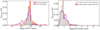 |
Fig. 1. Observed properties of our selected sample of galaxies and comparison to the global released VANDELS data. Left: apparent magnitude (Sextractor MAGAUTO) of our data in the i-band. Right: S/N measurements; at 1070–1170 Å restframe in red and at a fixed observed wavelength (6000–7400 Å) in purple. In the former case the median S/N is 0.97. |
3. Method
3.1. The SPARTAN tool
To estimate the IGM transmission towards our galaxies we use the SPARTAN tool which is able to fit both photometry and spectroscopic data. In this paper we use the capability of SPARTAN to fit spectroscopic dataset and photometric dataset separately. This single data type fitting follows the same recipe as other codes used in the literature (e.g. Salim et al. 2007; Thomas et al. 2017b). For a given object and a single template the χ2 and associated probability are estimated with:
![Mathematical equation: $$ \begin{aligned} \chi ^{2} = \sum _{i=1}^{N}\frac{(F_{\mathrm{obs},i}-A_{i}F_{\mathrm{syn},i})^{2}}{\sigma _{i}^{2}};\;\; P=\exp \left[-\frac{1}{2}\left(\chi ^{2}-\chi ^{2}_{\rm min}\right) \right] ,\end{aligned} $$](/articles/aa/full_html/2020/02/aa35925-19/aa35925-19-eq1.gif) (1)
(1)
where N, Fobs, i, Fsyn, i, σi, Ai and  stand for the number of observed data points, the flux of the data point itself, the synthetic template value at the same wavelength, the observed error associated to Fobs, i, the normalisation factor applied to the template, and the minimum χ2 of the library of templates, respectively. The latter is used to set the maximum of the probability distribution to unity. From the properties of the exponential function this is only a normalisation factor and does not change the values of the estimated parameters or their errors. The set of probability values (second part of Eq. (1)) is then used to create the probability distribution function (PDF, whose integral is normalised to unity) for each parameter to be estimated. From the PDF we create the cumulative distribution function (CDF) where the measured value of the parameter is taken where CDF(X) = 0.5 and the errors on this measurement correspond to the value of the parameter for which CDF = 0.05 and 0.95.
The photometric fitting process is performed as follows. The set of synthetic templates is redshifted to the redshift of the fitted galaxies and then normalised in one pre-defined band. For the photometric fitting we performed in this paper this normalisation is applied in the i-band. Following this normalisation, SPARTAN convolves the normalised template with all the photometric bandpasses available for the observed galaxy. Finally, the relations in Eq. (1) are applied to estimate the physical parameters of the observed galaxy and their associated errors.
When dealing with spectroscopic data, the general principle of the fitting process is similar that described immediately above. Nevertheless, this type of data allows for a different normalisation method. SPARTAN has to normalise the redshifted template to the observed spectrum. As for the photometry, we can consider a photometric filter and estimate the magnitude in the same filter from the spectrum itself. This magnitude serves as a normalisation to all the templates. This approach, widely used in the literature with photometric datasets, uses normalisation that is always done in a given photometric band (e.g. the i-band). As a result, each galaxy is normalised to the template in a different rest-frame region and all the galaxies are not treated in a similar manner. The spectroscopy opens allows for a new redshift-dependent method of normalisation. This method uses an emission-line-free region available in the spectrum. There is a region between 1070 and 1170 Å (rest-frame) in the UV spectrum of distant galaxies that is free from strong spectral lines. When fitting a UV spectrum at z = 4.5, this spectral region is shifted at 5885–6435 Å. SPARTAN computes a spectro-photometric point in this region directly in the template and in the data using a box filter of the size of this region. This box-magnitude is then used to normalise the template to the observed spectrum. At higher redshifts, such as z = 5.0 for example, this spectral region is at a redder wavelength (6420–7020 Å) and this observed-frame region is used to perform the normalisation as well. This new method of normalisation has the advantage of being consistent from one object to another. Moreover, as it is used in an emission-line-free region, it relies less on the emission line physics of the templates. Here we use the latter redshift-dependent normalisation method and we perform the normalisation in the region 1070–1170 Å (restframe). This region was chosen because once redshifted it provides a wide window for S/N estimation (∼500Å at z = 3.87 and ∼750Å at z = 6.5), it is free of strong emission lines, and considering the VIMOS wavelength window, it is one of the only sufficiently wide wavelength ranges available across the redshift range we consider.
3.2. Intergalactic-medium models and Tr(Lyα) definition
To estimate the IGM transmission we must be able to fit it. For years, the IGM transmission was fixed at a single value at a given redshift most often using the M95 model that provides a single transmission curve at a given redshift. Therefore, it was assumed that at a given redshift, the lines of sight of objects observed at a different position in the sky are populated by hydrogen clouds with the same properties. In M95, the author provides an estimate of the 1σ dispersion and, as mentioned in Sect. 1, this can vary from 20 to 70% at z = 3.5. Additionally, it was shown that this dispersion around the mean IGM could produce better photometric redshift (Furusawa et al. 2000). Therefore, we proposed in our previous paper the use of a set of empirical models that can reproduce this dispersion in the IGM transmission (Thomas et al. 2017a, hereafter T17). We summarise here how these templates were constructed. To test different lines of sight during the spectral energy distribution (SED) fitting we constructed six additional templates around the mean of M06. These additional models were built considering the ±1 sigma variation of M95 IGM models (see Fig. 3a in M95 paper at z = 3.5) which we propagated at any redshift. Finally, to explore more possibilities, we created, again from this ±1 sigma variation, the ±0.5σ and ±1.5σ. As a result, the IGM can be chosen from the set of seven discrete values at any redshift and this allows us to use the IGM as a free parameter in our fitting procedure and to explore a larger range of IGM transmission. At z = 3.0 the IGM transmission ranges from 20 to 100% while at z = 5.0 it ranges from 5 to 50%. As an example, we show in Fig. 2 the set of extinction curves at z = 4.0. In this paper we aim at computing the Lyα Transmission, Tr(Lyα), which is determined as the mean transmission between 1070 Å and 1170 Å computed on the transmission curve itself and shown in Fig. 2 as the area in grey. In the case of SPARTAN we use the PDF of Tr(Lyα) to estimate the value of the parameter, as described in Sect. 3.
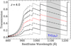 |
Fig. 2. Example of IGM transmission curves at z = 4.0. The red curve is from M06 Prescription while the black curves represent the augmented prescription from Thomas et al. (2017a). The latter allows us to span possible transmission from ∼15% to ∼90% at this redshift. The grey area shows where we compute the Lyα transmission. |
Finally, we emphasise that the IGM models we use here, while based on simulations, are also empirical (in the additional curves we use). More recent models include more components in the simulations such as the inclusion of the CGM (Steidel et al. 2018; Kakiichi & Dijkstra 2018). We will compare these different prescriptions in a future paper. It is also worth noting that the general shape of the curves is the same from one model to another while it can vary from one LOS to another depending on the presence of absorbers. In T17, we compared the results of the fit using the templates presented here and real Lyman α forest simulation (Bautista et al. 2015) and found that there was very good agreement in the resulting measurement of the Lyα transmission.
4. Dust content of z > 4 galaxies
In Thomas et al. (2017a) we identified a potential strong degeneracy between the estimates of the dust content of the galaxy and the IGM transmission prescription. This degeneracy is more prominent at z > 4. In other words, the same data can be fitted with high values of both dust extinction and IGM transmission or lower values for both parameters. This is due to the small wavelength range available from UV spectra for fitting that is not able to constrain the dust content of the galaxy. In order to address this problem in the present study, we measure the IGM transmission in a two-step process. First, we estimate the dust content of each galaxy in our sample using the photometric data presented in Sect. 2. We fit the SED over a broader wavelength range than the spectra including NIR data, providing robust constraints on dust extinction. We then estimate Tr(Lyα), keeping the E(B − V) value fixed to the one measured during the photometric-fitting process.
For this two-step fitting process we use the following parameter space. We use Bruzual & Charlot (2003) models with a Chabrier (2003) initial mass function. The stellar-phase metallicity ranges from subsolar (0.2 Z⊙ and 0.4 Z⊙) to solar (1.0 Z⊙). We assume a star formation history prescription that is exponentially delayed with a timescale parameter, τ, ranging from 0.1 to 1.0 Gyr. The ages range from 1 Myr to 3 Gyr in 24 steps. It is worth noting that this range of age is further limited by the age of the Universe at the redshift that is considered during the fit. The emission lines are added to the template following the work of Schaerer & de Barros (2009) that adds nebular continuum and emission using the conversion from ionizing photons to Hβ luminosity. Other emission lines are then added using line ratio from Anders & Fritze-v Alvensleben (2003). This first step is made to estimate the dust extinction. Therefore, in this section we use four different dust extinction curves1: the classical starburst (SB) galaxy prescription from Calzetti et al. (2000) with an extrapolation, the Small Magellanic Cloud (SMC) from Prevot et al. (1984), the prescription for the Large Magellanic Cloud (LMC) from Fitzpatrick (1986) and finally the prescription for the Milky Way (MW) from Allen (1976). All the curves are presented in Fig. 3 (top panel). For the photometric fitting, the E(B − V) parameter can vary from 0.0 to 0.39 (in 0.03 steps). Finally, the IGM prescription uses models developed in Thomas et al. (2017a) based on the M06 models (see previous section). The redshift used for this fitting is the spectroscopic redshift, zspec. Finally, it is worth noting that the IGM is estimated during this fitting process. These IGM measurements from the pure photometric fitting are discussed in Sect. 7.
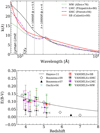 |
Fig. 3. Dust evolution from our 281 galaxies. Top panel: four different dust prescriptions used to estimate the dust extinction in our sample. In red we show the prescription from Calzetti et al. (2000), in black the prescription from Prevot et al. (1984) for the SMC, in violet the prescription from Fitzpatrick (1986) for the LMC, and in green for the Milky Way prescription by Allen (1976). Bottom panel: evolution with redshift of the dust attenuation in our selected sample of 281 galaxies from the photometric fitting for the four dust prescriptions shown in the top panel. Measurements report the mean and median absolute deviation for both the redshift and the E(B − V) values. We compare our results with previous measurements found in the literature at similar redshifts. The empty black diamonds are estimations from Bouwens et al. (2009), black triangles those from Bouwens et al. (2007), and light blue crosses show those from Ouchi et al. (2004). The dashed black line shows a fit from Hayes et al. (2011). We note that all the VANDELS estimations are at the same redshift; violet ones have been slightly shifted for clarity. |
The dust extinction measurements can be seen in Fig. 3 (bottom panel) which shows the evolution of the dust attenuation with redshift for our 281 selected galaxies and in Table 1 we report the measurements. Using the SB prescription we report mean values of E(B − V) = 0.11; 0.10; 0.10 and 0.08 at z = 3.99; 4.23; 4.59 and 5.15, respectively. Using the LMC curve the measurements are very similar and we obtain 0.11, 0.09, 0.08, and 0.05 at the same redshifts. The prescription of the SMC leads to a much weaker extinction at any redshift with 0.04, 0.03, 0.03, and 0.02 while the Milky-Way extinction from MW leads to slightly higher values of E(B − V) with 0.14, 0.11, 0.12 and 0.08. This is easily explained by the fact that for a fixed value of E(B − V) the curve of the SMC will lead to a much stronger extinction when studying UV-restframe galaxies (below 2000 Å), while the curve from the MW will give lower extinctions. The measurements obtained using SB, LMC, and MW are in good agreement with previous estimations at similar redshifts. Studying dropout-selected galaxies, Bouwens et al. (2009) reported an E(B − V) measurement of 0.14 at z ∼ 3.8 while E(B − V) = 0.095 at z = 5.0. At similar redshift, Ouchi et al. (2004) used Lyman-break galaxies in the range 3.5 < z < 5.2 and measured E(B − V) = 0.075 at z = 4.7. It is worth mentioning that SB-like laws have been supported by other studies in the literature (e.g. McLure et al. 2018b). On the contrary, the measurements using SMC are in strong disagreement with previous measurements from the literature, as reported in Scoville et al. (2015) and Fudamoto et al. (2017). In the remainder of the paper, we use both SB and MW models (LMC being very close to the SB) and see how this influences the measurements of the IGM.
Measurements of E(B − V) from the fit of photometry only using four different dust prescriptions.
5. Tr(Lyα) towards z > 4 galaxies
In the preceding section we measured the dust content of our galaxies; we now move towards the estimation of the IGM transmission with the spectral fit. In order to estimate this latter we constrain the spectral fit of our VANDELS spectroscopic data fixing the E(B − V) to that measured during the fit of the photometric data. We consider individual E(B − V) values for each of our galaxies and do not use the average values presented in Fig. 3. The other parameters, such as age or metallicity, are still free to vary and the parameter ranges correspond to those of the fit of Sect. 4. Examples of spectral fits of VANDELS galaxies are presented in Fig. 4 at various redshifts. These show that SPARTAN accurately reproduces the UV continuum of our galaxies at all wavelengths. It is worth mentioning that we can see that the Lyα is poorly reproduced. As presented in the previous section, the emission lines are added using line ratios and are therefore not fitted individually. Our results remain the same if we mask out the line during the fit.
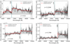 |
Fig. 4. Example of fits of VANDELS galaxies at redshift z > 4. In each plot the spectrum is shown by the black line while the best fit produced by SPARTAN is given in red. We indicate the position of the Lyα line and the redshift for each spectrum. |
Results on the measurement of Tr(Lyα) are presented in Fig. 5 where we show the distributions of the Lyman α transmission in four redshift bins: 3.85 < z < 4.1, 4.1 < z < 4.4, 4.4 < z < 4.8, and at z > 4.8. We also display the evolution of this quantity with redshift as compared with previous measurements in the literature (we take uneven binning to ensure a maximum number of galaxies in each bin). Table 2 provides the measurements for each bin. We estimated the Lyα transmission in these four redshift bins. Using the SB dust attenuation, this quantity goes from Tr(Lyα) = 0.55 at z = 3.99 with a large standard deviation of 0.14 to Tr(Lyα) = 0.29 at z = 5.15 with a standard deviation of 0.11. The standard error of the mean is small and is below 0.02 at any redshift. The measurements using the MW dust curve are similar, and are also similar to measurements done with QSOs at similar redshifts. Becker et al. (2013) measured Tr(Lyα) = 0.59 at z = 3.70 and Tr(Lyα) ∼ 0.35 at z ∼ 4.8. This shows that even at high redshift we are able to reproduce equivalent measurements with galaxies. Comparing our results to theoretical predictions, we find that we are in good agreement with the M06 models that predict Tr(Lyα) = 0.39 at z = 4.6 and Tr(Lyα) = 0.25 at z = 5.15. We note that our measurements are in partial disagreement with our previous measurements at z > 4 from the VUDS galaxies. At z = 4.23, the difference from our previous measurement is more than 10% and reaches 20% at z > 4.5. Nevertheless, as reported in Thomas et al. (2017a), these high values of Tr(Lyα) could actually be corrected limiting the E(B − V) to low values. Therefore, the method we employed in the present paper with an estimation of the E(B − V) value before the spectral fit seems to correct for this degeneracy.
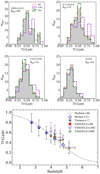 |
Fig. 5. Lyman α transmission (Tr(Lyα)) as a function of redshift. The top four first small plots show the distributions of the transmission in four redshift bins 3.85 < z < 4.1, 4.1 < z < 4.4, 4.4 < z < 4.8, and z > 4.8 for each dust prescription. We indicate the number of galaxies entering in the distribution in each of these plots. The bottom plots display the evolution of the transmission with redshift. Our measurements are indicated in red for SB, green for MW, and violet for LMC. We show the measurements for QSOs in blue from Becker et al. (2013), measurements for high redshift galaxies from the VIMOS Ultra Deep Survey (VUDS, Thomas et al. 2017a, in black), and the theoretical prediction from Meiksin (2006) represented with the black dashed line. |
Measurements of the Tr(Lyα) from our study.
More importantly we report a large standard deviation of Tr(Lyα) for all our measured points, going from 0.14 at z = 3.99 to 0.11 at z = 5.15. This is in good agreement with our previous study and confirms that the IGM should be treated as a free parameter during the fitting process. Surprisingly, we find that the measured values using the LMC prescription are above the measurements with the other prescription with a difference that peaks at +0.08 at z = 4.23 while the highest redshift point is in good agreement with the other dust solutions. We try to investigate these differences in the following section.
6. Averaged spectra
Finally, we analyse the averaged spectra of the population of our selected galaxies. We build two stack spectra that are constructed based on the IGM transmission as measured in our VANDELS galaxies: one where we select all the galaxies with a transmission higher than the mean curve given by M06, and one where all the galaxies have a transmission lower than the mean curve. Each stack spectrum is constructed using the specstack2 program (Thomas 2019a) which works as follows. For a given stack we de-redshift all the individual spectra and normalise them in a region redward of the Lyα line free of emission or absorption lines; in this case between the SiII(λ1260) and OI(λ1303) absorption line. We then re-grid all the spectra in a common wavelength grid. Finally, at a given wavelength, we compute the mean of all the fluxes using a sigma-clipping method (at 3σ).
The averaged spectra are presented in Fig. 6 (using the fits made with SB). This figure shows that below Lyα at 1215 Å, there is a non-negligible variation in flux. The low-transmission stacked spectra are on average ∼30% dimmer than the stacked spectra with high IGM transmission. This means that at z > 4, the standard deviation of the IGM is very important, and that IGM transmission should be treated as a free parameter when studying galaxies at such high redshift. It is also worth mentioning that the average redshift of the two stacks is slightly different. For the stacks with IGM below the mean, the average redshift is z ∼ 4.36, while it is z ∼ 4.60 for the galaxies with an IGM higher than the mean. Consequently, the difference might be even higher than what we measure here. Finally, the figure shows that the spectra beyond the Lyα line are very similar. A few absorption lines are stronger in the case of high IGM transmission (e.g. OI and SiIV) but others present similar strengths (e.g. SiII and CII). It is therefore difficult to make any robust conclusions concerning this aspect.
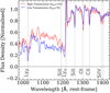 |
Fig. 6. Averaged spectra. We display two stack spectra. In blue we show the average of all the spectra (79) with IGM transmission lower than the mean. The mean redshift in these spectrum is ∼4.36. In red we show the average of all the spectra (101) with IGM transmission higher than the mean, with a mean redshift of ∼4.60. The stack spectra have been made with the specstack program (Thomas 2019a). |
7. Discussion
7.1. Flag system and flux calibration
As mentioned in Sect. 2 we did not take into account the flag system when selecting our galaxies. However we checked whether or not our results are impacted by the presence of lower quality redshift measurements that could potentially indicate the presence of low-redshift interlopers. We removed the redshift flags “1” and “9” and results are reported in Table 2 and displayed in Fig. 7. The only notable difference is the last point that is at a slightly lower redshift at z = 4.98 instead of z = 5.15, indicating that the highest measured redshifts are of a lower quality than the lower redshift sample. This is because the redshift is often measured thanks to the presence of the Lyα which leads to a redshift quality flag of “9”. For the other points, the change in Tr(Lyα) is less than 0.01, which represents a less-than 2% difference. We conclude that including redshift flags 1, 2, and 9 has almost no impact on the global results of our study.
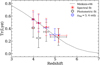 |
Fig. 7. Intergalactic medium transmission Tr(Lyα) as a function of redshift from different estimations. In red we show our final results, as presented in Fig. 5, in blue we show the evolution of Tr(Lyα) for galaxies with a redshift flag of 3 or 4 only, and in black we show the results of the photometric fit only. |
As reported in Pentericci et al. (2018), the very bluest part of the VANDELS spectra was suffering from a systematic mismatch with the broadband photometry available for the sources. The underlying cause of this is still under investigation but for the moment (and at the time of DR1 and 2) we have implemented an empirically derived correction to the spectra. This effect could in principle be relevant for the objects belonging to the first redshift bin. For this reason we repeated the same measurements in the two first bins using uncorrected spectra and measure an IGM transmission of 0.55 at z = 3.99 with a standard deviation of 0.16, and 0.51 at z = 4.23 with a standard deviation 0.16 as well. This shows that the effects of spectral corrections are negligible and lower than 5%.
7.2. Discussion on the method
We also measured the IGM transmission from the first-pass photometric fitting performed in Sect. 4 (with free dust extinction parameter). Results are reported in Fig. 7 and Table 2. As expected the measurements are in strong disagreement with the results from the spectral fit. The difference is on average −0.11 towards low Tr(Lyα) values. This difference can reach up to 0.24 at z = 4.23. This shows that the use of photometric data alone to constrain the IGM transmission is not efficient. Photometric data are less numerous and we have access to less bands to constrain the fit. Indeed, photometry provides us with a data point every 500 or 1000 Å. Spectroscopy on the other hand brings much more constraints, with one data point every ∼4 Å.
We finally test the difference in dust extinction estimation (E(B − V), using SB) and Tr(Lyα) if we do not fix the dust extinction during the spectral fit. Leaving it free, the dust extinction that we measure increases with respect to the photometric fitting of Sect. 4. The measurement of E(B − V) gives 0.12, 0.13, 0.15, and 0.12 at z = 3.99, 4.23, 4.59, and z = 5.15. While we are still in the dispersion, this corresponds to a change of 10% at z = 4.05 and more than 50% at z = 5.15. Considering Tr(Lyα), the measurements are slightly different from the main results of our paper; the first point at z = 3.99 remains the same while the second and third measurements are higher when leaving the dust free with Tr(Lyα) = 0.51 at z = 4.23 and Tr(Lyα) = 0.44 at z = 4.59. This makes a difference of between 0.03 and 0.02, respectively. The strongest difference is for the last point where ΔTr(Lyα) = 0.05. This behaviour is expected. If the dust content goes towards higher E(B − V) values (i.e. more extinction), the IGM transmission must compensate this extinction going towards higher Tr(Lyα) values (higher transmission). This behaviour was already noted in our previous study.
7.3. Intergalactic medium template resampling
In the previous sections we used seven IGM transmission curves at any redshift. We want to know now if the sampling of our prescription has an influence on the final measurements. To this aim, we created a new IGM prescription, not composed of seven possible transmissions but of 31 transmission templates. We keep the same range but add intermediate curves, each at multiples of 0.1σ from 0.1 to 1.5σ. The transmission curves at z = 4.0 can be seen in Fig. 8 (top).
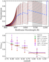 |
Fig. 8. Top: intergalactic medium transmission at z = 4 in the case where we finely sample the IGM templates and consider 31 transmission curves instead of 7. The blue curve shows the average M06 prescription and the grey region locates the region where we measure Tr(Lyα). Bottom: comparison of the Tr(Lyα) in the cases where we use 7 curves or 31 curves. |
Using this fine-sampled prescription we recompute the dust and the IGM transmission using all three dust prescriptions. The results are displayed in Fig. 8. This comparison shows that the difference is minimal. Using the SB dust attenuation, the difference between using 7 or 31 or the other is less than 0.1%. For the two other dust prescriptions, the main difference is for the point at the lowest redshift where the difference reaches 4% for the LMC and 5% for the MW prescription. We can conclude that the prescription with seven curves seems to be adequately detailed and adding more curves does not substantially change the results.
8. Conclusion
This paper reports the study of the IGM transmission Tr(Lyα) at z > 4. We measured the IGM transmission from the spectra of 281 galaxies coming from the VANDELS public survey carried out by the VIMOS instrument at the VLT. Galaxies have been observed for up to ∼80 h, thus providing unprecedented spectral depth. Using a previously published IGM transmission prescription for template fitting studies we used the SPARTAN fitting tool to compute the IGM transmission. We summarise our results below:
-
In order to tackle the dust-IGM degeneracy that was discovered in a previous study, we first estimated the dust content in our galaxies with a pure photometric fitting technique. We estimated the mean E(B − V) at z > 4 and found that it ranges from 0.11 at z = 3.99 to 0.08 at z = 5.15. These measurements are similar to previous measurements reported in the literature.
-
Using individual measurements of E(B − V) as constraints, we use the SPARTAN software to perform the spectral fitting of our galaxies. From this fitting, we extract the values of Tr(Lyα) at various redshifts. Tr(Lyα) decreases from Tr(Lyα) = 0.53 at z = 3.99 to Tr(Lyα) = 0.28 at z = 5.15. These results closely match the measurements from the study of QSOs and from theoretical predictions. This reinforces the idea that high-redshift galaxies can be used to estimate the IGM.
-
Even more importantly, the 1σ scatter of Tr(Lyα) is large at any redshift; it is higher than 0.1 and equivalent to the standard deviation reported for QSOs.
-
As expected we find that the IGM transmission measurements are sensitive to the choice of dust attenuation prescription.
-
We test whether our results are sensitive to the redshift flag system in place in VANDELS and find that the differences are minimal.
-
Due to a lack of observational constraints, the measurements coming from a pure photometric fitting are not able to reproduce the results from the spectral fitting and from the literature.
-
Finally, we compute the IGM transmission leaving the dust extinction as a free parameter and we confirm the presence of dust/IGM degeneracy. In this latter case, the dust extinction goes towards higher values that are in tension with measurements found in the literature. This is then compensated by a higher IGM transmission.
Finally, it is worth reiterating that there are multiple IGM models in the literature and these should be tested against real data. High-redshift data samples are becoming large enough to perform statistically significant tests of these models. This will be studied in a paper that is in preparation.
Acknowledgments
The authors wish to thank the referee we provided us with very insightful comments that improved a lot the paper.
References
- Allen, C. W. 1976, Astrophysical Quantities (London: Athlone) [Google Scholar]
- Anders, P., & Fritze-v Alvensleben, U. 2003, A&A, 401, 1063 [NASA ADS] [CrossRef] [EDP Sciences] [Google Scholar]
- Bautista, J. E., Bailey, S., Font-Ribera, A., et al. 2015, JCAP, 2015, 060 [NASA ADS] [CrossRef] [Google Scholar]
- Becker, G. D., Hewett, P. C., Worseck, G., & Prochaska, J. X. 2013, MNRAS, 430, 2067 [NASA ADS] [CrossRef] [Google Scholar]
- Bolton, J. S., Haehnelt, M. G., Viel, M., Springel, V. 2005, MNRAS, 357, 1178 [NASA ADS] [CrossRef] [Google Scholar]
- Bouwens, R. J., Illingworth, G. D., Franx, M., & Ford, H. 2007, ApJ, 670, 928 [NASA ADS] [CrossRef] [Google Scholar]
- Bouwens, R. J., Illingworth, G. D., Franx, M., et al. 2009, ApJ, 705, 936 [NASA ADS] [CrossRef] [Google Scholar]
- Bruzual, G., & Charlot, S. 2003, MNRAS, 344, 1000 [NASA ADS] [CrossRef] [Google Scholar]
- Calzetti, D., Armus, L., Bohlin, R. C., et al. 2000, ApJ, 533, 682 [NASA ADS] [CrossRef] [Google Scholar]
- Cardamone, C. N., van Dokkum, P. G., Urry, C. M., et al. 2010, ApJS, 189, 270 [NASA ADS] [CrossRef] [Google Scholar]
- Cen, R., Miralda-Escudé, J., Ostriker, J. P., & Rauch, M. 1994, ApJ, 437, L9 [Google Scholar]
- Chabrier, G. 2003, PASP, 115, 763 [NASA ADS] [CrossRef] [Google Scholar]
- Faucher-Giguère, C.-A., Prochaska, J. X., Lidz, A.,Hernquist, L., Zaldarriaga, M. 2008, APJ, 681, 831 [Google Scholar]
- Fitzpatrick, E. L. 1986, AJ, 92, 1068 [NASA ADS] [CrossRef] [Google Scholar]
- Fudamoto, Y., Oesch, P. A., Schinnerer, E., et al. 2017, MNRAS, 472, 483 [NASA ADS] [CrossRef] [Google Scholar]
- Furusawa, H., Shimasaku, K., Doi, M., & Okamura, S. 2000, ApJ, 534, 624 [NASA ADS] [CrossRef] [Google Scholar]
- Furusawa, H., Kosugi, G., Akiyama, M., et al. 2008, ApJS, 176, 1 [NASA ADS] [CrossRef] [Google Scholar]
- Furusawa, H., Kashikawa, N., Kobayashi, M. A. R., et al. 2016, ApJ, 822, 46 [NASA ADS] [CrossRef] [Google Scholar]
- Galametz, A., Grazian, A., Fontana, A., et al. 2013, ApJS, 206, 10 [NASA ADS] [CrossRef] [Google Scholar]
- Garilli, B., Fumana, M., Franzetti, P., et al. 2010, PASP, 122, 827 [NASA ADS] [CrossRef] [Google Scholar]
- Garilli, B., Paioro, L., Scodeggio, M., et al. 2012, PASP, 124, 1232 [NASA ADS] [CrossRef] [Google Scholar]
- Guo, Y., Ferguson, H. C., Giavalisco, M., et al. 2013, ApJS, 207, 24 [NASA ADS] [CrossRef] [Google Scholar]
- Haardt, F., & Madau, P. 1996, APJ, 461, 20 [Google Scholar]
- Hayes, M., Schaerer, D., Östlin, G., et al. 2011, ApJ, 730, 8 [NASA ADS] [CrossRef] [Google Scholar]
- Hsieh, B.-C., Wang, W.-H., Hsieh, C.-C., et al. 2012, ApJS, 203, 23 [NASA ADS] [CrossRef] [Google Scholar]
- Inoue, A. K., Shimizu, I., Iwata, I., & Tanaka, M. 2014, MNRAS, 442, 1805 [NASA ADS] [CrossRef] [Google Scholar]
- Jarvis, M. J., Bonfield, D. G., Bruce, V. A., et al. 2013, MNRAS, 428, 1281 [NASA ADS] [CrossRef] [Google Scholar]
- Kakiichi, K., & Dijkstra, M. 2018, MNRAS, 480, 5140 [NASA ADS] [Google Scholar]
- Le Fèvre, O., Saisse, M., Mancini, D., et al. 2003, in Instrument Design and Performance for Optical/Infrared Ground-based Telescopes, eds. M. Iye, & A. F. M. Moorwood, Proc SPIE, 4841, 1670 [CrossRef] [Google Scholar]
- Le Fèvre, O., Tasca, L. A. M., Cassata, P., et al. 2015, A&A, 576, A79 [NASA ADS] [CrossRef] [EDP Sciences] [Google Scholar]
- Madau, P. 1995, ApJ, 441, 18 [NASA ADS] [CrossRef] [Google Scholar]
- McLure, R. J., Pentericci, L., Cimatti, A., et al. 2018a, MNRAS, 479, 25 [NASA ADS] [Google Scholar]
- McLure, R. J., Dunlop, J. S., Cullen, F., et al. 2018b, MNRAS, 476, 3991 [NASA ADS] [CrossRef] [Google Scholar]
- Meiksin, A. 2006, MNRAS, 365, 807 [NASA ADS] [CrossRef] [Google Scholar]
- Meiksin, A., & White, M. 2004, MNRAS, 350, 1107 [NASA ADS] [CrossRef] [Google Scholar]
- Oke, J. B., & Gunn, J. E. 1983, ApJ, 266, 713 [NASA ADS] [CrossRef] [Google Scholar]
- Ouchi, M., Shimasaku, K., Okamura, S., et al. 2004, ApJ, 611, 660 [NASA ADS] [CrossRef] [Google Scholar]
- Pentericci, L., McLure, R. J., Garilli, B., et al. 2018, A&A, 616, A174 [NASA ADS] [CrossRef] [EDP Sciences] [Google Scholar]
- Prevot, M. L., Lequeux, J., Maurice, E., Prevot, L., & Rocca-Volmerange, B. 1984, A&A, 132, 389 [Google Scholar]
- Rauch, M., Miralda-Escudè, J., Sargent, W. L. W., et al. 1997, APJ, 489, 7 [NASA ADS] [CrossRef] [Google Scholar]
- Salim, S., Rich, R. M., Charlot, S., et al. 2007, ApJS, 173, 267 [NASA ADS] [CrossRef] [Google Scholar]
- Schaerer, D., & de Barros, S. 2009, A&A, 502, 423 [NASA ADS] [CrossRef] [EDP Sciences] [Google Scholar]
- Scoville, N., Faisst, A., Capak, P., et al. 2015, ApJ, 800, 108 [NASA ADS] [CrossRef] [Google Scholar]
- Sobral, D., Best, P. N., Matsuda, Y., et al. 2012, MNRAS, 420, 1926 [NASA ADS] [CrossRef] [Google Scholar]
- Steidel, C. C., Bogosavljević, M., Shapley, A. E., et al. 2018, ApJ, 869, 123 [NASA ADS] [CrossRef] [Google Scholar]
- Stoehr, F., White, R., Smith, M., et al. 2008, in DER_SNR: A Simple & General Spectroscopic Signal-to-Noise Measurement Algorithm, eds. R. W. Argyle, P. S. Bunclark, & J. R. Lewis, ASP Conf. Ser., 394, 505 [Google Scholar]
- Thomas, R. 2019a, Astrophysic Source Code Library [record ascl:1904.018] [Google Scholar]
- Thomas, R. 2019b, Astrophysic Source Code Library [record ascl:1901.007] [Google Scholar]
- Thomas, R. 2019c, https://doi.org/10.5281/zenodo.2626564 [Google Scholar]
- Thomas, R. 2019d, https://doi.org/10.5281/zenodo.2587874 [Google Scholar]
- Thomas, R. 2019e, J. Open Source Softw., 4, 1259 [Google Scholar]
- Thomas, R., Le Fèvre, O., Le Brun, V., et al. 2017a, A&A, 597, A88 [NASA ADS] [CrossRef] [EDP Sciences] [Google Scholar]
- Thomas, R., Le Fèvre, O., Scodeggio, M., et al. 2017b, A&A, 602, A35 [NASA ADS] [CrossRef] [EDP Sciences] [Google Scholar]
- Yoshii, Y., & Peterson, B. A. 1994, ApJ, 436, 551 [NASA ADS] [CrossRef] [Google Scholar]
Appendix A: Reproducibility
Reproducibility has become a crucial aspect of modern research with the use of software and codes. Sharing codes and methods in papers is as important as sharing results. In this appendix we aim at providing this crucial information. Table A.1 lists the availability of the data-related and technique-related aspects of our work. Each point is detailed in the following paragraph.
Summary of the reproducibility of this work.
– As presented in Sect. 2, the VANDELS survey is a public spectroscopic survey. As such all the data are already publicly available and freely available from the ESO archive facility3.
– The SPARTAN tool is available on GITHUB and comes with all the inputs needed to run the code. The version released at this moment allows a separate fit on the photometry and on the spectroscopy, as used in this paper. The version used in this paper is version 0.4.44. The final version will be presented in a paper in preparation (Thomas et al., in prep).
– In addition, the main Python packages used during this work are public: catalogue query module catscii (v1.2, Thomas 2019d), catalogue matching algorithm catmatch (v1.3 Thomas 2019c), our fits display library dfitspy (v19.3.4, Thomas 2019e), the spectrum stacking program specstack (v19.4, Thomas 2019a) and our plotting tool, Photon (v0.3.2, Thomas 2019b). They are all available in the main python package index repository (pypi).
All Tables
Measurements of E(B − V) from the fit of photometry only using four different dust prescriptions.
All Figures
|
Fig. 1. Observed properties of our selected sample of galaxies and comparison to the global released VANDELS data. Left: apparent magnitude (Sextractor MAGAUTO) of our data in the i-band. Right: S/N measurements; at 1070–1170 Å restframe in red and at a fixed observed wavelength (6000–7400 Å) in purple. In the former case the median S/N is 0.97. |
| In the text | |
|
Fig. 2. Example of IGM transmission curves at z = 4.0. The red curve is from M06 Prescription while the black curves represent the augmented prescription from Thomas et al. (2017a). The latter allows us to span possible transmission from ∼15% to ∼90% at this redshift. The grey area shows where we compute the Lyα transmission. |
| In the text | |
|
Fig. 3. Dust evolution from our 281 galaxies. Top panel: four different dust prescriptions used to estimate the dust extinction in our sample. In red we show the prescription from Calzetti et al. (2000), in black the prescription from Prevot et al. (1984) for the SMC, in violet the prescription from Fitzpatrick (1986) for the LMC, and in green for the Milky Way prescription by Allen (1976). Bottom panel: evolution with redshift of the dust attenuation in our selected sample of 281 galaxies from the photometric fitting for the four dust prescriptions shown in the top panel. Measurements report the mean and median absolute deviation for both the redshift and the E(B − V) values. We compare our results with previous measurements found in the literature at similar redshifts. The empty black diamonds are estimations from Bouwens et al. (2009), black triangles those from Bouwens et al. (2007), and light blue crosses show those from Ouchi et al. (2004). The dashed black line shows a fit from Hayes et al. (2011). We note that all the VANDELS estimations are at the same redshift; violet ones have been slightly shifted for clarity. |
| In the text | |
|
Fig. 4. Example of fits of VANDELS galaxies at redshift z > 4. In each plot the spectrum is shown by the black line while the best fit produced by SPARTAN is given in red. We indicate the position of the Lyα line and the redshift for each spectrum. |
| In the text | |
|
Fig. 5. Lyman α transmission (Tr(Lyα)) as a function of redshift. The top four first small plots show the distributions of the transmission in four redshift bins 3.85 < z < 4.1, 4.1 < z < 4.4, 4.4 < z < 4.8, and z > 4.8 for each dust prescription. We indicate the number of galaxies entering in the distribution in each of these plots. The bottom plots display the evolution of the transmission with redshift. Our measurements are indicated in red for SB, green for MW, and violet for LMC. We show the measurements for QSOs in blue from Becker et al. (2013), measurements for high redshift galaxies from the VIMOS Ultra Deep Survey (VUDS, Thomas et al. 2017a, in black), and the theoretical prediction from Meiksin (2006) represented with the black dashed line. |
| In the text | |
|
Fig. 6. Averaged spectra. We display two stack spectra. In blue we show the average of all the spectra (79) with IGM transmission lower than the mean. The mean redshift in these spectrum is ∼4.36. In red we show the average of all the spectra (101) with IGM transmission higher than the mean, with a mean redshift of ∼4.60. The stack spectra have been made with the specstack program (Thomas 2019a). |
| In the text | |
|
Fig. 7. Intergalactic medium transmission Tr(Lyα) as a function of redshift from different estimations. In red we show our final results, as presented in Fig. 5, in blue we show the evolution of Tr(Lyα) for galaxies with a redshift flag of 3 or 4 only, and in black we show the results of the photometric fit only. |
| In the text | |
|
Fig. 8. Top: intergalactic medium transmission at z = 4 in the case where we finely sample the IGM templates and consider 31 transmission curves instead of 7. The blue curve shows the average M06 prescription and the grey region locates the region where we measure Tr(Lyα). Bottom: comparison of the Tr(Lyα) in the cases where we use 7 curves or 31 curves. |
| In the text | |
Current usage metrics show cumulative count of Article Views (full-text article views including HTML views, PDF and ePub downloads, according to the available data) and Abstracts Views on Vision4Press platform.
Data correspond to usage on the plateform after 2015. The current usage metrics is available 48-96 hours after online publication and is updated daily on week days.
Initial download of the metrics may take a while.