| Issue |
A&A
Volume 633, January 2020
|
|
|---|---|---|
| Article Number | A90 | |
| Number of page(s) | 14 | |
| Section | Extragalactic astronomy | |
| DOI | https://doi.org/10.1051/0004-6361/201936872 | |
| Published online | 15 January 2020 | |
The ALPINE-ALMA [C II] survey: Star-formation-driven outflows and circumgalactic enrichment in the early Universe
1
Observatoire de Genève, Universitè de Genève, 51 Ch. des Maillettes, 1290 Versoix, Switzerland
e-mail: This email address is being protected from spambots. You need JavaScript enabled to view it.
2
Cavendish Laboratory, University of Cambridge, 19 J. J. Thomson Ave., Cambridge CB3 0HE, UK
3
Kavli Institute for Cosmology, University of Cambridge, Madingley Road, Cambridge CB3 0HA, UK
4
Aix Marseille Univ, CNRS, CNES, LAM, Marseille, France
5
Osservatorio di Astrofisica e Scienza dello Spazio – Istituto Nazionale di Astrofisica, Via Gobetti 93/3, 40129 Bologna, Italy
6
University of Bologna, Department of Physics and Astronomy (DIFA), Via Gobetti 93/2, 40129 Bologna, Italy
7
Institute for Cosmic Ray Research, The University of Tokyo, Kashiwa-no-ha, Kashiwa 277-8582, Japan
8
Department of Astronomy, School of Science, The University of Tokyo, 7-3-1 Hongo, Bunkyo, Tokyo 113-0033, Japan
9
IPAC, California Institute of Technology, 1200 East California Boulevard, Pasadena, CA 91125, USA
10
University of Padova, Department of Physics and Astronomy, Vicolo Osservatorio 3, 35122 Padova, Italy
11
Kavli Institute for the Physics and Mathematics of the Universe (Kavli IPMU, WPI), The University of Tokyo, Kashiwa 277-8583, Japan
12
Caltech Optical Observatories, Cahill Center for Astronomy and Astrophysics, 1200 East California Boulevard, Pasadena, CA 91125, USA
13
Centro de Astronomia (CITEVA), Universidad de Antofagasta, Avenida Angamos 601, Antofagasta, Chile
14
Instituto de Fisica y Astronomia, Universidad de Valparaiso, Gran Bretana 1111, Playa Ancha, Valparaiso, Chile
15
Department of Physics and Astronomy, University of Massachusetts, Amherst, MA 01003, USA
16
Department of Physics, University of California, Davis, One Shields Ave., Davis, CA 95616, USA
17
Department of Astronomy, University of Florida, 211 Bryant Space Sciences Center, Gainesville, FL 32611, USA
18
Cosmic Dawn Center (DAWN), Denmark
19
Niels Bohr Institute, University of Copenhagen, Lyngbyvej 2, 2100 Copenhagen, Denmark
20
Leiden Observatory, Leiden University, PO Box 9500, 2300 RA Leiden, The Netherlands
Received:
8
October
2019
Accepted:
15
November
2019
Abstract
We study the efficiency of galactic feedback in the early Universe by stacking the [C II] 158 μm emission in a large sample of normal star-forming galaxies at 4 < z < 6 from the ALMA Large Program to INvestigate [C II] at Early times (ALPINE) survey. Searching for typical signatures of outflows in the high-velocity tails of the stacked [C II] profile, we observe (i) deviations from a single-component Gaussian model in the combined residuals and (ii) broad emission in the stacked [C II] spectrum, with velocities of |v|≲500 km s−1. The significance of these features increases when stacking the subset of galaxies with star formation rates (SFRs) higher than the median (SFRmed = 25 M⊙ yr−1), thus confirming their star-formation-driven nature. The estimated mass outflow rates are comparable to the SFRs, yielding mass-loading factors of the order of unity (similarly to local star-forming galaxies), suggesting that star-formation-driven feedback may play a lesser role in quenching galaxies at z > 4. From the stacking analysis of the datacubes, we find that the combined [C II] core emission (|v|< 200 km s−1) of the higher-SFR galaxies is extended on physical sizes of ∼30 kpc (diameter scale), well beyond the analogous [C II] core emission of lower-SFR galaxies and the stacked far-infrared continuum. The detection of such extended metal-enriched gas, likely tracing circumgalactic gas enriched by past outflows, corroborates previous similar studies, confirming that baryon cycle and gas exchanges with the circumgalactic medium are at work in normal star-forming galaxies already at early epochs.
Key words: galaxies: evolution / galaxies: formation / galaxies: high-redshift / galaxies: ISM / ISM: jets and outflows / galaxies: star formation
© ESO 2020
1. Introduction
Current models of galaxy formation widely agree on the key importance of stellar feedback in regulating the evolution of galaxies over cosmic time. Massive stars (≳8 M⊙) emit copious high-energy photons during their lifetimes and inject energy and momentum in the surrounding gas through supernova (SN) explosions in the final stage of their evolution (see a review by Woosley et al. 2002). These mechanisms can heat the gas and drive turbulent motions in the interstellar medium (ISM; e.g., Dekel & Silk 1986; Mac Low & Ferrara 1999; Hopkins et al. 2012, 2014), reducing the star formation efficiency to the observed typical low values of a few percent of the free-fall time (e.g., Kennicutt 1998; Krumholz & McKee 2005; Leroy et al. 2008, 2013; Bigiel et al. 2011). Stellar feedback is also often invoked to explain the observed discrepancy between the measured galaxy luminosity (or stellar mass, M⋆) function (LF) and the dark matter (DM) halo mass function predicted by the standard cosmological model (e.g., Benson et al. 2003; Silk & Mamon 2012; Behroozi et al. 2013). While the sharp exponential cut-off at the luminous end of the LF is usually ascribed to feedback from accreting black holes (BHs) in active galactic nuclei (AGNs; see e.g., Bower et al. 2006; Cattaneo et al. 2009; Fabian 2012), SN feedback is thought to be the dominant mechanism in shaping the flat slope at the low-mass end of the LF (e.g., Dekel & Silk 1986; Heckman et al. 1990; Hopkins et al. 2014). In particular, intense episodes of star formation induce powerful SN-driven winds, which can efficiently accelerate the gas to hundreds of kilometers per second (see e.g., Heckman & Thompson 2017) and eventually expel it from the disk, (i) suppressing the star formation rate (SFR; e.g., Somerville & Davé 2015; Hopkins et al. 2016; Hayward & Hopkins 2017), and (ii) enriching the circumgalactic and intergalactic medium (CGM and IGM) with heavy elements (e.g., Oppenheimer & Davé 2006; Oppenheimer et al. 2010; Pallottini et al. 2014).
Observational evidence of stellar feedback has increased over the years (see Veilleux et al. 2005; Erb 2015 for thorough reviews). A widely adopted method to trace the kinematics of cold and warm outflowing gas consists in measuring the blueshift of metal absorption resonant lines in the rest-frame ultraviolet (UV) and optical bands, with respect to the systemic redshift (usually measured through strong optical emission lines). This technique has been extensively employed to characterise star-formation-driven outflows in both local (e.g., Arribas et al. 2014; Chisholm et al. 2015, 2016, 2017; Cicone et al. 2016) and distant galaxies, up to z ≲ 3 − 4 (e.g., Shapley et al. 2003; Steidel et al. 2004, 2010; Rubin et al. 2010, 2014; Talia et al. 2012, 2017; Heckman et al. 2015).
At higher redshifts, approaching the epoch of reionization, detecting outflows through absorption-line spectroscopy becomes challenging, mainly because of (i) increasingly weaker metal absorption features, and (ii) large uncertainties on the systemic redshifts, which cannot be obtained from Lyα, whose line profile is strongly affected by intergalactic absorption and radiative transfer effects. A possible way to overcome such limitations comes from the growing number of recent Atacama Large Millimeter/submillimeter Array (ALMA) observations of bright far-infrared (FIR) lines, such as for example [C II] 158 μm (hereafter [C II]) and [O III] 88 μm at z > 4 (see e.g., Wagg et al. 2012; Capak et al. 2015; Maiolino et al. 2015; Inoue et al. 2016; Bradač et al. 2017; Hashimoto et al. 2018; Carniani et al. 2018; Matthee et al. 2019). For instance, combining the redshift determined from [C II] with deep observed-frame optical spectra taken at DEIMOS/Keck, Sugahara et al. (2019) constructed a high-signal-to-noise-ratio (high-S/N) composite far-UV spectrum of seven Lyman break galaxies (LBGs) at z = 5 − 6 (Riechers et al. 2014; Capak et al. 2015). Sugahara et al. (2019) find central outflow velocities (i.e., values measured at the line center corresponding to the bulk motion of the gas) of vout ≳ 400 km s−1 and maximum outflow velocities of about 800 km s−1, highlighting an increase (by a factor > 3) with respect to galaxies at lower redshifts (see Sugahara et al. 2017).
To probe star-formation-driven outflows in the early Universe, an alternative method to rest-frame FUV absorption line spectroscopy consists in studying the broad wings in the high-velocity tails of FIR-line spectra, similarly to what is commonly done for luminous AGN-driven outflows (see e.g., Maiolino et al. 2012; Feruglio et al. 2018; Decarli et al. 2018; Bischetti et al. 2019; Stanley et al. 2019). Unfortunately, even significant investments of ALMA time (≲1 h; see e.g., Capak et al. 2015) do not provide sufficiently good spectra to analyze in detail the weak broad components of FIR lines in individual “normal”1 star-forming galaxies at z > 4, and stacking of large samples would be needed. Some indications of the discovery potential of the FIR-line stacking analysis come from recent results by Gallerani et al. (2018), who found flux excesses at about v ± 500 km s−1 in the stacked residual [C II]-spectrum of a small sample of nine galaxies at z ∼ 5 − 6 (Capak et al. 2015), likely ascribed to broad wings tracing star-formation-driven outflows.
Aiming to improve our understanding of galactic feedback at early epochs, we explore the efficiency of star-formation-driven outflows through a stacking analysis of [C II] emission lines in a large sample of normal galaxies at 4 < z < 6, from our ALMA Large Program to Investigate C+ at Early Times (ALPINE) survey (Le Fèvre et al. 2019a; Béthermin et al., in prep.; Faisst et al. 2019; see a short description of the survey in Sect. 2). On the one hand, the diversity of ALPINE galaxies (almost 2 dex in SFR and M⋆ are spanned across the main sequence) and the wealth of ancillary multi-wavelength photometric data (from UV to FIR) enable us to investigate primary dependencies of stellar outflows on galaxy physical properties. On the other hand, the large statistics provided (the number of [C II]-detected galaxies used for the stacking is approximately six-fold higher than similar previous studies; see Gallerani et al. 2018) yields enough sensitivity to (i) map the spatial extension of the outflowing gas and (ii) constrain the circumgalactic enrichment on scales of a few tens of kiloparsec, providing new critical pieces of information on the baryon cycling physics that drives the evolution of high-z galaxies.
The paper is organized as follows. In Sect. 2 we describe the ALPINE survey and the data-reduction process, while in Sect. 3 we describe the methods of our analysis and report the results. Section 4 contains a discussion on the implications of our findings, and Conclusions are summarized in Sect. 5.
Throughout the paper, we assume a flat Universe with Ωm = 0.3, ΩΛ = 0.7 and H0 = 70 km s−1 Mpc−1, and adopt a Chabrier initial mass function (IMF; Chabrier 2003).
2. Sample and observations
ALPINE is an ALMA large program (PI: Le Fèvre et al. 2019a; Béthermin et al., in prep.; Faisst et al. 2019) designed to measure [C II] and the FIR-continuum emission for a representative sample of 118 normal galaxies at z = [4.4 − 5.8]. This enables extensive studies of the ISM and dust properties, as well as kinematics, and dust-obscured star formation in a representative population of high-z galaxies, with template-fitting derived SFR ≳ 5 M⊙ yr−1 and stellar masses in the range M⋆ ∼ 108.5 − 1011 M⊙ (see Fig. 1). All galaxies have reliable optical spectroscopic redshifts coming from extensive campaigns at the Very Large Telescope (VUDS: Le Fèvre et al. 2015; Tasca et al. 2017) and Keck (Keck-COSMOS: Hasinger et al. 2018; Capak et al., in prep.), and benefit from a wealth of ancillary multi-wavelength photometric data (from UV to FIR; see Faisst et al., in prep.). This makes ALPINE one of the currently largest panchromatic samples to study the physical properties of normal high-z galaxies (see a discussion in Le Fèvre et al. 2019a; Faisst et al. 2019).
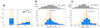 |
Fig. 1. Redshift (a), SFR (b), and M⋆ (c) distributions of galaxies in the ALPINE survey (orange) and galaxies in our final sample (blue), drawn from ALPINE and used in this work (see Sect. 3.1.2). For comparison, in panels b and c we show the SFR and M⋆ distributions of all COSMOS galaxies with photometric redshift in the ALPINE range z = [4.4 − 5.8] (from Laigle et al. 2016). The gap in the redshift distribution is due to the original ALPINE sample selection, tailored to avoid a prominent atmospheric absorption at ∼325 GHz in ALMA band 7. The black dashed lines in panels b and c represent the median SFR and Mstar of galaxies in our ALPINE-drawn sample. |
The overall ALMA observational strategy/setup and details on the data reduction steps (including data quality assessment) are comprehensively discussed in Béthermin et al. (in prep.); however, a short summary of relevant information is reported here. ALMA observations were carried out in Band 7 during Cycles 5 and 6, and completed in February 2019. Each target was observed for between 20 min and 1 h of exposure time, with phases centered at the rest-frame UV positions of the sources. One spectral window was centered on the [C II] expected frequencies, according to the spectroscopic redshifts extracted from UV spectra, while other side bands were used for continuum measurements. The data were calibrated using the Common Astronomy Software Applications package (CASA; McMullin et al. 2007), version 5.4.0, and additional flagging of bad antennae was performed in a few cases (see Béthermin et al., in prep.). Continuum maps were obtained running the CASA task clean (multi-frequency synthesis mode) over the line-free visibilities in all spectral windows, while [C II] datacubes were generated from the continuum-subtracted visibilities, with 500 iterations and a S/N threshold of σclean = 3 in the clean algorithm. We chose a natural weighting of the visibilities, a common pixel size of 0.15″ and a common spectral bin of 25 km s−1 (which is the best compromise in terms of number of spectral elements to resolve the line and S/N per channel). The median sensitivity (in the spectral regions close to [C II] frequencies) reached by the cubes in our sample is ∼0.35 mJy beam−1 for a 25 km s−1 spectral channel, while the overall distribution ranges between 0.2 and 0.55 mJy beam−1 per channel with the same velocity binning. Such a variation (notwithstanding similar integration times) is mainly driven by the redshift range covered by our targets and the evolving atmospheric transmissivity function in ALMA Band 7 (see Béthermin et al., in prep.). The typical angular resolution of the final products, computed as the average circularized beam axis, is 0.9″ (∼5.2 − 6 kpc in the redshift range z = 4.4 − 5.8), with values ranging 0.8″ − 1″. In Béthermin et al. (in prep.), we discuss in detail the methods adopted to extract continuum and [C II] information from ALPINE observations, while we refer to other forthcoming works for an overview of ALPINE-related results. The data set consists of 75 robustly [C II]-detected galaxies with S/N > 3.5 (i.e., the threshold at which our simulations indicate a 95% reliability; see Béthermin et al., in prep.) calculated as the ratio between peak fluxes and rms in optimally extracted2 [C II] velocity-integrated maps. We note that, as discussed in Sect. 3, in this work we exclude from our analysis ∼30% of the sample, consisting of merging systems.
3. Analysis and results
[C II] is the brightest line in the FIR spectra of star-forming galaxies and has been exploited to trace AGN-driven outflows revealed by the presence of broad wings in the spectra of luminous high-z QSOs (see e.g., Maiolino et al. 2012; Cicone et al. 2015; Janssen et al. 2016; Feruglio et al. 2018; Decarli et al. 2018; Bischetti et al. 2019; Stanley et al. 2019). In normal galaxies, where outflows are expected to be powered to a greater extent by stellar feedback than by AGN activity, broad wings are expected to be less prominent and weaker (see, e.g., a review by Heckman & Thompson 2017); therefore, even in the deepest currently available [C II] observations at z ≳ 4, the sensitivity is generally not adequate to detect weak broad components in individual objects (e.g., Capak et al. 2015; Maiolino et al. 2015; Gallerani et al. 2018; Fujimoto et al. 2019).
To explore the efficiency of galactic feedback at play in normal star-forming galaxies in the early Universe, we performed a stacking analysis of the [C II] emission in a sample of galaxies (see Sect. 3.1.2) drawn from the ALPINE survey (see Sect. 2). The stacking technique enables us to substantially increase the sensitivity in the combined spectra and cubes. It therefore holds a significant discovery potential as shown in Bischetti et al. (2019) and Gallerani et al. (2018), who successfully carried out the stacking of a QSO sample at 4.5 < z < 7, and a small sample of normal galaxies at z ∼ 5, respectively. In the following we describe the methods used to extract, align, and stack [C II] spectra and cubes of our galaxies, and report the results.
3.1. Methods and stacking analysis
Our analysis is based on three different procedures (described in the following paragraphs), each of them providing complementary information:
-
(1)
Stacking of the residuals, computed by subtracting a single-component Gaussian fit to each [C II] spectrum (Sect. 3.2). This procedure is needed to test whether or not a single-Gaussian component is sufficient to describe (on average) our [C II] spectra.
-
(2)
Stacking of the [C II] spectra (Sect. 3.3) to verify the improvement gained in describing the combined spectrum with a two-component Gaussian model, and to compute the typical outflow properties (e.g., velocity and mass of the neutral atomic gas).
-
(3)
Stacking of the [C II] cubes (Sect. 3.4), to obtain information on the typical spatial distribution of the [C II] emission, both at low- and high-velocities.
3.1.1. Extraction of spectra and alignment
To extract the [C II] spectra of our galaxies, we used 2D apertures defined by the pixels contained within the 2σ-levels of our optimally extracted [C II] velocity-integrated maps (see Béthermin et al., in prep.). Rather than adopting a common fixed aperture, this has the advantage of taking into account variable morphologies and/or extensions of the gas, in order to include most of the flux coming from the total [C II]-emitting region, and to minimize the addition of noise. However, as discussed in Sect. 3.3, we also tested fixed and smaller apertures.
Before stacking, we align the spectral axes of both spectra and cubes according to their [C II] observed frequencies: we set as a common “zero-velocity” reference the 25 km s−1-sized channel or slice centered (after interpolation) on the centroid frequency of the Gaussian fit. The resulting distribution of the number of objects per spectral element (as shown in the top panels of Figs. 2 and 3) is not uniform along the full velocity range and declines starting from a few hundred kilometres per second around the line, and is halved at about ±1000 km s−1. These effects are mainly due to: (i) the exclusion of a few spectral channels flagged by the pipeline during the reduction steps, and more importantly (ii) spectral offsets between the observed [C II] redshifts and the expected redshifts as derived from rest-frame UV spectra originally used to center the spectral windows (see Béthermin et al., in prep. and Cassata et al., in prep., for technical details and a physical interpretation of the velocity offsets, respectively).
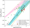 |
Fig. 2. Top: histogram containing the number of objects per channel contributing to the stacked flux. Central lower panel: variance-weighted stacked [C II] residuals from a single-Gaussian fit in spectral bins of 25 km s−1 (75 km s−1). The green solid lines at ±800 km s−1 enclose the velocity range excluded for the estimation of spectral noise, while the blue dashed lines represent the spectral rms at ±1σ. Channels in violet represent the channels in the velocity range enclosed by the outermost peaks at ≥3σ in the 75 km s−1-binned stacked residuals. This helps in visualizing the velocity interval affected by flux excesses. |
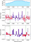 |
Fig. 3. Same description as in Fig. 2. Here the stacked residuals are shown for the low-SFR (a), and the high-SFR (b) groups, respectively. While the stacked residuals are consistent with the noise in the low-SFR subsample, significant (> 4σ) peaks of flux excess are detected for high-SFR galaxies. |
We also spatially align the [C II] cubes, centering them on the brightest pixel of [C II] velocity-integrated maps. This procedure is preferred to choosing the phase center (coincident with the centroid of rest-frame UV positions of the sources) as a common spatial reference point, since a few sources show small spatial offsets (< 1″, whose physical interpretation will be discussed in another paper) between the [C II] and optical images centroids3.
3.1.2. Exclusion of possible contaminants
As explained in Sect. 3.1 and discussed in the following paragraphs, we are interested in revealing deviations from a single-component Gaussian model and flux excesses in the high-velocity tails of the stacked spectra and cubes possibly due to SF-driven winds. Since these effects may be mimicked by companion galaxies and satellites in interacting systems (see discussions in e.g., Gallerani et al. 2018; Fujimoto et al. 2019; Pallottini et al. 2019), we excluded from our analysis 25 objects (corresponding to ∼30% of the [C II]-detected ALPINE sample) with signs of ongoing major or minor mergers; for those systems a proper spatial or spectral deblending cannot be performed and any attempt does not guarantee the removal of possible contamination. Such selection is based on a morpho-kinematic classification, described in detail in Le Fèvre et al. (2019a) and performed combining information from the ancillary multi-wavelength photometry and the ALMA products (e.g., velocity-integrated [C II] maps, 2D kinematics maps, and position-velocity diagrams; see Jones et al., in prep.). We note that our exclusion of interacting systems does not prevent the sample from being somehow still contaminated by unresolved, HST/ALMA undetected, faint satellites4. As discussed in the following sections, some arguments suggest that this effect should not be significant, however a more robust solution to this issue is yet to be provided and may require future deeper and higher-resolution observations.
The final sample, drawn from ALPINE and used in this work, consists of 50 normal star-forming galaxies at redshift 4.4 < z < 5.8, with SFR ∼ 5 − 600 M⊙ yr−1 and log(M⋆/M⊙) ∼ 9 − 11 (see Fig. 1). Stellar masses and star formation rates are derived using a rich set of available ancillary data, including ground-based imaging observations from rest-frame UV to the optical, HST observations in the rest-frame UV, and Spitzer coverage above the Balmer break. We used Bruzual & Charlot (2003) composite stellar population template fitting, using the LePhare code (Arnouts et al. 1999; Ilbert et al. 2006) with a large range in stellar ages, metallicities, and dust reddening. For further details we refer to Faisst et al. (in prep.), where a focused discussion on the ALPINE ancillary dataset and fitted physical properties (including characterization of the systematic uncertainties resulting from modeling assumptions) will be presented.
3.2. Combining the residuals
Prior to searching for signatures of star-formation-driven outflows in the high-velocity tails of the stacked [C II] spectrum, we checked the null hypothesis that the [C II] line profiles of our galaxies are well (and completely) described by a single-Gaussian model. We performed a simple standard procedure (see e.g., Gallerani et al. 2018) described as follows:
-
(i)
we fit a single-Gaussian profile to each [C II] spectrum (where the peak flux, center velocity5, and full width at half maximum (FWHM) are free parameters), and compute the model value Gi, in each independent 25 km s−1-sized spectral bin i;
-
(ii)
for each spectrum we compute the residuals Ri, by subtracting in each channel the best-fitting Gaussian model Gi from the observed flux Fi, i.e., Ri = Fi − Gi;
-
(iii)
we combine the residuals performing a variance-weighted stacking:
 (1)
(1)where N is the number of galaxies contributing to each velocity bin, and the weighting factor wk is defined as
 , where σk is the spectral noise associated with the spectrum k. We compute σk as the root mean square (rms) of the noise contained in each spectrum excluding channels in the velocity range [ − 800 : + 800] km s−1 around the center, to avoid the [C II] emission line of the galaxies themselves. We found this range to be an optimal compromise between (i) having a large number of independent spectral bins to use for the determination of noise and (ii) conservatively excluding the velocity range usually found to be affected by stellar outflows. The effectiveness of this choice is probed a posteriori by our own results, since (as discussed in the following) no significant residuals are found at |v|> 600 − 700 km s−1.
In Fig. 2 we show the resulting stacked residuals,  , where for each spectral channel i, we report in the top panel the number of sources contributing to the corresponding flux. In the velocity range v ∼ [ − 500 : + 500] km s−1 we find peaks of flux excess with significance > 3σ (where σ is computed as the ratio between
  and σk) in single velocity bins (see violet bins, whose definition is reported in the caption of Fig. 2), while the flux distribution in the stacked residuals at larger velocities (|v|> 600 km s−1) is completely consistent with the noise. To facilitate the interpretation and improve the visualization, we re-bin the stacked residuals in channels of 75 km s−1 (averaging over three contiguous spectral elements), revealing an increase of the flux excess significance up to 4σ in the velocity range v ∼ [ − 500 : + 500] km s−1.
We note that if our [C II] spectra were completely described by a single-Gaussian profile, the resulting flux from the stacked residuals should be simply consistent with random noise over the full velocity range.
To explore the origin of such observed deviations from a single-Gaussian profile and probe any connection with stellar feedback, we repeat the analysis described above dividing our sample into two SFR-defined bins, and analyzing each of them individually. Specifically, we use the median SFR of galaxies in our sample (SFRmed = 25 M⊙ yr−1; see Fig. 1b) as the threshold to create two equally populated subsamples of low-SFR galaxies (SFR < 25 M⊙ yr−1) and high-SFR galaxies (SFR ≥ 25 M⊙ yr−1).
We find that the stacked residuals of low-SFR galaxies do not show any clear sign of significant flux-excess over the entire velocity range, as shown in Fig. 3a. Channels at v ∼ [ − 500 : + 500] km s−1 (where positive signal is detected when stacking the full sample; see Fig. 2) are noise-dominated, with only few channels exceeding 2σ.
The flux excess at |v|≲500 km s−1 in the stacked residuals of high-SFR galaxies is more distinct than in the stacked residuals of the full sample, with (i) a larger number of connected velocity bins at S/N > 3σ, and (ii) peaks reaching an increased significance of 4σ (5σ) in the 25 km s−1 (75 km s−1)-binned spectrum (see Fig. 3b). At lower velocities, v ∼ [ − 300 : + 300] km s−1, the residuals appear flatter, with some weak positive residuals around the zero and weak symmetric negative peaks at about v ± 250 km s−1 (see lower panel of Fig. 3b)6.
Therefore, the most star-forming galaxies in our sample contribute more to the deviation from a single-Gaussian profile, indicating a possible connection (on average) between the amount of SFR and the observed deviation from a single-component Gaussian profile in the [C II] spectra of high-z normal galaxies. Altogether, these findings suggest that star formation (or, more appropriately, star-formation-driven mechanisms) is likely to be responsible for producing the observed flux excess at the high-velocity tails of the stacked residuals.
Any contribution from rotating galaxies?
While dispersion-dominated galaxies exhibit single-peak spectra, the double-horned profiles of rotating disks (see e.g., Begeman 1989; Daddi et al. 2010; de Blok et al. 2016; Kohandel et al. 2019) are not well described by a single Gaussian. In addition, evidence for rotating disks has been found at high redshift (e.g., De Breuck et al. 2014; Jones et al. 2017; Talia et al. 2018; Smit et al. 2018). Therefore, it is conceivable that the presence of rotating disks in our sample may contribute to the deviation from a single-Gaussian (see e.g., Kohandel et al. 2019) and to the production of the symmetric residuals seen in Fig. 3. However, we note that large rotational velocities of |v|∼500 km s−1 have been observed only in bright submillimeter galaxies (SMGs) and AGN-host galaxies, with intense SFRs ≳ 1000 M⊙ yr−1 and very broad FWHMs ≳ 800 km s−1 (see e.g., Carniani et al. 2013; Jones et al. 2017; Talia et al. 2018), and are unlikely to be produced by normal star-forming rotating galaxies (the median FWHM of [C II] profiles in our high-SFR galaxies is ∼250 km s−1).
To further explore this argument, we use 3DBAROLO (a tool for fitting 3D tilted-ring models to emission-line datacubes that takes into account the effect of beam smearing; see Di Teodoro & Fraternali 2015) to build kinematic models of five galaxies classified as rotators in the high-SFR group, for which we have enough independent spatial elements to obtain robust fits (Jones et al., in prep.). The criteria adopted to classify rotators in ALPINE are discussed in detail in Le Fèvre et al. (2019a) (see also Sect. 3.1.2), and mainly require (i) smooth transitions between intensity channel maps, (ii) clear gradients in velocity field maps, (iii) tilted (straight) position–velocity diagrams projected along the major (minor) axis, (iv) possible double-horned profiles in the spectra and, (v) single components in ancillary photometric data. We then repeat the residuals stack of our high-SFR galaxies, but now, for the five ALPINE rotators modeled with 3DBAROLO, we calculate Ri, k (see Eq. (1)) by subtracting the tilted-ring fit from the observed spectra rather than the Gaussian model. The result is shown in Fig. 4: while residuals resulting from the kinematic modeling (limited by our ∼1″ spatial resolution) are indeed visible (see green channels), these are more concentrated toward the common reference center, only affecting the velocity range v ∼ [ − 225 : + 275] km s−1 (see gray shaded region). This test suggests that the effect of unresolved kinematics in the spectra of our normal rotating galaxies should not have a significant impact on the residuals observed at |v|≲500 km s−1, whose origin should be ascribed to other mechanisms, as discussed below.
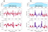 |
Fig. 4. Similar to the central panel of Fig. 3b, the 25 km s−1-binned stacked [C II] residuals of the high-SFR group are shown. However, here, for the five rotators in the subsample, Ri, k (see Eq. (1)) is calculated by subtracting a kinematic model to the observed spectra. We color in green the channels where the residuals left by the tilted-ring fit are non-null, specifically in the velocity range v ∼ [ − 225 : + 275] km s−1, marked by the gray shaded region. |
3.3. Stacking the spectra
In Sect. 3.2 we discussed that a single-Gaussian component is not sufficient to correctly model (on average) the [C II] spectra of a representative (see M⋆ and SFR distributions in Fig. 1) population of high-z normal galaxies (Fig. 2). In particular, we found that the deviation from a single-Gaussian model is related to the SFR, with high(low)-significance flux excess found in the stacked residuals of high(low)-SFR galaxies (Fig. 3). Interestingly, in line with previous similar works (e.g., Gallerani et al. 2018), most of the positive signal revealed in the stacked residuals of highly star-forming galaxies arises from almost symmetric high-velocity tails (see Fig. 3b), specifically at velocities consistent with those observed through UV spectroscopy in the outflowing gas accelerated by stellar feedback at similar redshifts (e.g., Sugahara et al. 2019; see a discussion in Sect. 1). This suggests that the observed flux excess can be ascribed to SFR-driven outflows. However, to corroborate this hypothesis, we need to test whether a two-component Gaussian model, that is, a combination of a narrow and a broad component (with the latter tracing the outflowing gas; see Sect. 3), can better describe our observations.
We therefore performed a variance-weighted stacking of the [C II] spectra of galaxies in our sample to compute (and compare) the residuals of single-Gaussian and two-component Gaussian best fits. In analogy with Eq. (1), each ith channel of the stacked spectrum  is defined as:
 (2)
(2)
where Si, k is the [C II] spectrum of the kth galaxy, and the weighting factor  is calculated as described in Sect. 3.2.
In Fig. 5a we show the [C II] spectrum resulting from the stacking of our full sample (with a spectral element binning of 25 km s−1) along with the single- and two-component Gaussian best fits. As for the figures in Sect. 3.2, a histogram reporting the number of objects per channel contributing to the corresponding flux is shown on the top panel. The stacked [C II] spectrum appears to be clearly characterized by weak (less than 10% of the line peak-flux) broad wings at velocities of a few hundred kilometers per second (see inset in Fig. 5a). We find that while a single-Gaussian fit produces significant positive residuals at v ∼ ±[300 : 500] km s−1 (in agreement with results from Sect. 3.2), a two-component Gaussian fit can accurately describe the stacked spectrum, leaving residuals that are reasonably consistent with simple noise (no peaks exist at > 2σ; see Fig. 5b). Our best fit with a two-Gaussian model results in a combination of a narrow component and a relatively less prominent broad component, in agreement with typical line profiles observed in the presence of outflows at low-z or in galaxies hosting an AGN (see a discussion in Sect. 1). Both the narrow and broad Gaussian components are centered at the stacked [C II] line peak (vcen ∼ 0 ± 10 km s−1). We measure a FWHM = 233 ± 15 km s−1 for the narrow component, and a FWHM = 531 ± 90 km s−1 for the broad component7, where the uncertainties are estimated through a bootstrap analysis, as described in the following paragraphs.
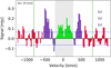 |
Fig. 5. a: variance-weighted stacked [C II] spectrum of all galaxies in our sample is shown, in velocity bins of 25 km s−1. The orange (blue) line shows the single-Gaussian (two-Gaussian) best-fit. The red and the green line represent the narrow and broad components of the two-Gaussian model, respectively. A zoom of the velocity range [ − 600 : + 600] km s−1 is shown in the inset. A histogram containing the number of objects per channel contributing to the stacking is shown in the top panel. b: residuals from the single-Gaussian (two-Gaussian) best-fit are shown in red (blue), in velocity bins of 50 km s−1. |
As done with the stacked residuals, we test the dependence of the average [C II] spectral line shape on the SFR, dividing our sample into two SFR bins as described in Sect. 3.2, and repeating the analysis in each group.
We find that the stacked [C II] spectrum of low-SFR galaxies (SFR < 25 M⊙ yr−1) does not show clear signs of broad wings (see Fig. 6a). As expected, given the different line shapes of the constituent spectra (which combine as a sum of Gaussians with different widths) and the larger number of free parameters, the residuals left by the two-component Gaussian best fit are lower than in the single-Gaussian case. However, the residuals produced by the single-Gaussian best fit are generally consistent with the noise (no peaks at ≳3σ), indicating that the stacked spectrum of the low-SFR galaxies can be sufficiently well described by a single-component Gaussian profile. Moreover, in this case the two-component Gaussian best fit is not determined by the expected combination of a narrow and (less prominent) broad component, and therefore does not provide a meaningful result.
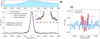 |
Fig. 6. Same description as in Fig. 5. In this case the stacked [C II] spectrum and corresponding residuals from a single- and two-Gaussian best-fits are shown for the low-SFR (a), and the high-SFR (b) subsamples, individually. |
The stacked [C II] spectrum of high-SFR galaxies (SFR > 25 M⊙ yr−1) shows clear signs of broad wings on the high-velocity tails, at v ± ∼500 km s−1 (see Fig. 6b). The single-Gaussian best fit leaves significant residuals (with peaks exceeding 4σ) in the velocity range v ∼ ±[300 : 500] km s−1, more prominent than the residuals found in the combined spectrum from the full sample. On the other hand, the two-component Gaussian best fit, resulting in the combination of a narrow (FWHM = 251 ± 10 km s−1) and a broad (FWHM = 684 ± 75 km s−1) component (see Table 1), produces residuals that are fully consistent with the noise.
Median SFRs of full and high-SFR (sub)samples are summarized, along with the FWHMs of both narrow and broad Gaussian components.
These findings do not prove the absence of a broad component (i.e., a possible signature of outflows) in the stacked spectrum of the low-SFR subsample. Indeed, since [C II] is generally fainter in low-SFR galaxies (see e.g., Capak et al. 2015; Carniani et al. 2018; Matthee et al. 2019; Schaerer et al., in prep.), we might expect this feature to be less evident and most likely below the detection limit. On the other hand, since the noise level in both stacks is comparable (given the same number of galaxies in the two bins), we can safely argue that high-SFR galaxies are (on average) characterized by larger and more prominent broad components in their [C II] spectra.
We performed a bootstrap analysis to estimate the possible effect of contamination from a few individual sources in the (sub)samples where we found evidence of broad wings. In Figs. 7a and b, we show the FWHM distributions of both narrow and broad components obtained with the bootstrap technique for the full sample and the subsample of highly star-forming galaxies, respectively. The two panels show that for both narrow and broad components, the peaks of FWHM distributions are highly consistent with the values reported in the analysis described above (without any random replacement), indicating that no obvious dominance by a small number of galaxies is affecting our results. To improve the reliability of our measurements, we adopt the σ of the bootstrapped FWHM distributions (see labels in Fig. 7) as uncertainties on the FWHM values of the stacked spectra reported above (see also Table 1).
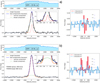 |
Fig. 7. Distribution of the FWHM of narrow (red histograms) and broad (green histograms) components obtained with a bootstrap analysis for the full sample (a) and the high-SFR group (b). The dashed lines represent the median values of the distribution. |
We also repeated the stacking of high-SFR galaxies by combining the [C II] spectra extracted from a fixed 4 × 4 pixel-sized aperture (diameter of 0.6″, i.e., slightly more than half of the averaged circularized beam) centered on the brightest pixels of the velocity-integrated [C II] maps. Apart from a small difference in terms of absolute signal, we do not find clear deviations from the stacked spectrum shown in Fig. 6b, further suggesting that a possible contamination from faint satellites (at least on scales comparable with the beam) does not contribute significantly in building-up the observed broad component.
While the FWHM of the broad component that we measure (FWHM < 700 km s−1; see Table 1) is much smaller than that observed in typical high-z QSOs (i.e., FWHM ≳ 2000 km s−1; see Maiolino et al. 2012; Cicone et al. 2015; Bischetti et al. 2019), we note that some contribution to the [C II] broadening may come from (i) winds powered by gas accretion onto moderately massive black holes or, (ii) strongly obscured AGNs, especially in the high-SFR group. One of the objectives of our survey will indeed be to characterize the AGN activity of ALPINE galaxies using, for instance, (i) X-ray stacking diagnostics and (ii) stacked UV spectra to constrain the Type II-AGN-sensitive lines (e.g., HeII-λ1640 Å and [CIII]-λ1908 Å; see e.g., Nakajima et al. 2018; Le Fèvre et al. 2019b). In addition to this, JWST will help in terms of resolved BPT diagram classification (Baldwin et al. 1981) and observations of broad Hα or [OIII]-λ5007 Å line emissions.
3.4. Stacking the cubes
As discussed in the previous sections, our stacking analysis of [C II] spectra shows that the significance of residuals from a single-Gaussian fit and broad wings on the high-velocity tails, at v ± ∼500 km s−1, increases with the SFR, indicating that star-formation-driven outflows are at play in high-z normal galaxies. To better characterize the outflow properties, we explored the morphologies and spatial extensions of both the core and high-velocity wings of the[C II] line. We combined the [C II] cubes of our galaxies Ci, spectrally and spatially aligned as discussed in Sect. 3.1.1, following a vector variance-weighted stacking:
 (3)
(3)
Equation (3) is a generalized version of Eq. (2) (see e.g., Fruchter & Hook 2002; Bischetti et al. 2019), where  is the stacked cube composed by i slices, Ci, k is the [C II] cube of the kth galaxy and wi, k is the weighting factor defined as
  . Here
  is defined as the spatial rms estimated from a large emission-free region at each ith slice of each kth galaxy, and allows us to account for any frequency-dependent noise variation in the [C II] cubes.
Following the same procedure described in Sects. 3.2 and 3.3, we performed the stacking analysis of [C II] cubes for both (i) the full sample and (ii) two groups of galaxies with SFR higher or lower than the median SFR in our sample, that is SFR ≶25 M⊙ yr−1. We then collapsed the spectral slices of the [C II] stacked cubes in the velocity ranges (i) [ − 200 : + 200] km s−1, and (ii) [ − 600 : − 200], [ + 200 : + 600] km s−1. Those ranges were specifically chosen to produce velocity-integrated flux maps of (i) the core of the [C II] emission, and (ii) the [C II] high-velocity tails, respectively. In Fig. 8 we show the central 8″ × 8″ regions of the flux maps from the stacked cubes.
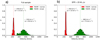 |
Fig. 8. Velocity-integrated [C II] flux maps (central 8″ × 8″ regions) are shown in different velocity ranges, from the combined cubes obtained by stacking (a) the full sample, (b) the low-SFR, and (c) the high-SFR groups. Left and right panels: representative of the high-velocity tails of the [C II] emission ([ − 600 : − 200] and [ + 200 : + 600] km s−1, respectively), while maps in the central panels trace the [C II] core ([ − 200 : + 200] km s−1). Significance levels of the black contours are reported below the panels of (a). The average synthesized beam is shown in the lower-left corners, while a reference size-scale of 15 kpc is reported at the bottom of each panel. The center of each panel is marked with a white cross. |
We find that [C II] emission is detected up to 4σ in the velocity-integrated maps at [ − 600 : − 200] and [ + 200 : + 600] km s−1 of the full sample, and up to 5σ in the high-SFR group. Only tentative detections (∼2σ) are revealed in the high-velocity tails of the low-SFR group (see side panels of Fig. 8). Where detected, the high-velocity [C II] emission is marginally resolved (compared with the average beam of the observations in the stack8), extending on beam-deconvolved9 angular sizes of ∼0.9″, corresponding to ∼6 kpc at zmed = 5 (the median redshift of our galaxies).
In the velocity-integrated image at [ − 200 : + 200] km s−1, which traces the core of line, we detect [C II] emission at exceptionally high significance in all our three (sub)samples, that is, ≳30σ in the full sample and high-SFR bin and ≳10σ in the low-SFR group (see central panels of Fig. 8). Interestingly, while in all three cases [C II] emission is fully resolved and extended on angular scales of > 2″ (> 15 kpc at zmed = 5), the core of [C II] line emission appears to be more extended for the high-SFR galaxies, with low-S/N (2σ) features extending up to angular scales of ≳3″, corresponding to about 20 kpc at zmed = 5.
To test the reliability of these results, we repeated the analysis carrying out a median stacking instead of the variance-weighted mean stacking described in Eq. (3). We do not find evident deviations, confirming that our findings are not affected by outliers in the distribution.
To constrain the typical extension of the stacked [C II] line core with higher accuracy and quantify its dependence on the SFR (as suggested by the flux maps in Fig. 8), we computed the circularly averaged radial profiles of surface brightness (SB) from the low-velocity [C II] flux maps of our stacked (sub)samples (see Fig. 9). We then compared them with the radial profiles of SB extracted from the stacked point spread function (PSF) image and the stacked FIR continuum; the former is obtained by stacking the ALMA PSF cubes of galaxies in our sample (using Eq. (3)) and by collapsing the channels at [ − 200 : + 200] km s−1, while the latter is obtained through a mean- and rms-weighted stack of the FIR-continuum images of the 23 ALPINE continuum-detected galaxies (∼90% of which belong to our high-SFR subsample; see details in Béthermin et al., in prep. and Khusanova et al., in prep.). Figure 9 shows that the radial profile of the stacked [C II] line core in the low-SFR group is slightly more extended than the average PSF radial profile. It extends similarly to the FIR continuum (deconvolved effective radii of ∼1.2″; ∼8 kpc at zmed = 5), suggesting that they are both tracing gas emitted on the same (galactic) scale.
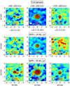 |
Fig. 9. Circularly averaged radial profiles computed in concentric 0.3″-binned annuli are shown for (i) the stacked PSF of our ALMA observations (black solid line for galaxies in our sample, and black dashed line for ALPINE continuum-detected galaxies), (ii) the stacked FIR continuum of 23 ALPINE continuum-detected galaxies (mostly belonging to the high-SFR group, see text; orange squares), and (iii) the stacked maps of [C II] cores ([ − 200 : + 200] km s−1) for galaxies in the low-SFR (green squares) and high-SFR (blue square) groups. Error bars are indicative of the ±1σ dispersion of fluxes in each annulus, while the thin dashed lines represent the Poissonian noise associated with the radial profiles10. |
On the other hand the radial profile of the stacked [C II] line core in the high-SFR subsample can be seen to extend well beyond the analogous emission from lower-SFR galaxies. The stacked FIR continuum, reaching a deconvolved effective radius of 2.3″, corresponds to a physical distance of ∼15 kpc at zmed = 5. While the relatively more compact profile of low-SFR galaxies could in principle be interpreted as an effect of limited sensitivity, we can safely argue that higher-SFR galaxies show larger [C II] fluxes on average on radial scales > 10 kpc.
Our statistical detection of a low-velocity [C II] emission extended on such large physical sizes (diameter scales of ∼30 kpc) suggests the existence of metal enriched circumgalactic halos surrounding main sequence high-z galaxies, confirming with larger statistics and significance the result obtained by Fujimoto et al. (2019), who found a 20 kpc (diameter scale) [C II] halo in the stacked cube of 18 galaxies at 5 < z < 7 (see their discussion for an overview of the theoretical mechanisms proposed to explain the extended emission). Since outflows of processed material are needed to enrich with carbon the primordial CGM of early systems (see Fujimoto et al. 2019), the detected [C II] halo is evidence of (i) past star-formation-driven outflows and (ii) gas mixing at play in the CGM of high-z normal star-forming galaxies (see a discussion in Sect. 4). We postpone further explorations of these findings to future papers, including, for example, analyses of the rest-frame UV continuum (Fujimoto et al., in prep.) and Lyα stacked emissions, as well as comparisons with tailored hydrodynamical simulations (e.g., Behrens et al. 2019; Pallottini et al. 2019; Mayer et al., in prep.).
4. Discussion
The stacking analysis of [C II] spectra and cubes of ALPINE galaxies described in Sect. 3 suggests that outflows are unequivocal in normal star-forming galaxies at 4 < z < 6 (see possible caveats in Sect. 3.1.2). Interestingly, we find that the intensity and the significance of [C II] emission in the broad wings at the high-velocity tails of the stacked spectra and cubes increases with the SFR, supporting the star-formation-induced nature of the observed outflows.
4.1. Mass outflow rate and efficiency of star-formation-driven outflows
To estimate the efficiency of star-formation-driven outflows at play in high-z galaxies, we calculated the mass outflow rate (Ṁout) following an approach similar to previous studies of outflows in the [C II] spectra of QSOs and normal galaxies (e.g., Maiolino et al. 2012; Cicone et al. 2015; Janssen et al. 2016; Gallerani et al. 2018; Bischetti et al. 2019).
We use the luminosity of the broad [C II] component to get an estimate of the outflowing atomic gas mass,  , adopting the relation from Hailey-Dunsheath et al. (2010):
![Mathematical equation: $$ \begin{aligned} \dfrac{M_{\rm out}^{\mathrm{atom}}}{{M}_\odot } =&0.77 \left( \dfrac{0.7\,L_{\mathrm{[C II]}}}{{L}_\odot } \right) \times \left( \dfrac{1.4\times 10^{-4}}{X_{\mathrm{C}^+}}\right) \nonumber \\&\times \dfrac{1+2 e^{-91\,\mathrm{K}/T} + n_{\mathrm{crit}}/n}{2 e^{-91\,\mathrm{K}/T}}, \end{aligned} $$](/articles/aa/full_html/2020/01/aa36872-19/aa36872-19-eq13.gif) (4)
(4)
where XC+ is the abundance of C+ per hydrogen atom, n is the gas number density, ncrit is the critical density of the [C II] 158 μm transition (i.e., ∼3 × 103 cm−3), and T is the gas temperature. This relation is derived under the assumption that most of the broad [C II] emission arises from atomic gas (see a discussion in Janssen et al. 2016); specifically, 70% of the total [C II] flux (corresponding to the factor 0.7 in the first parenthesis of Eq. (4)) arises from photodissociation regions (PDRs; e.g., Stacey et al. 1991, 2010), with only the remaining fraction arising from other ISM phases (see e.g., Cormier et al. 2012; Vallini et al. 2015, 2017; Lagache et al. 2018; Ferrara et al. 2019, for discussions on the relative contribution of various gas phases). It is also assumed that the [C II] emission is optically thin; this sets a lower limit on  since, in case of optically thick [C II], the actual outflowing gas mass would be larger. We use Eq. (4) assuming (i) a gas number density higher than ncrit (this approximation gives a lower limit on the mass of the atomic gas, as discussed in Maiolino et al. 2012), and (ii) a C+ abundance, XC+ ∼ 1.4 × 10⁻⁴, (Savage & Sembach 1996) and a gas temperature in the range T ∼ 60 − 200 K, both typical of PDRs (see e.g., Kaufman et al. 1999, 2006; Hollenbach & Tielens 1999; Wolfire et al. 2003). Applying Eq. (4) to the stacked [C II] spectra of our full and high-SFR (sub)samples (where broad components are detected) we infer a mass of the outflowing atomic gas,
  , for the full sample, and
  for the high-SFR subsample, where the errors reflect the explored range of T and the uncertainties on L[CII]. We then compute the atomic Ṁout assuming time-averaged expelled shells or clumps (Rupke et al. 2005; Gallerani et al. 2018):
 (5)
(5)
where:
-
vout is the typical velocity of the atomic outflowing gas traced by [C II]. We adopt vout ∼ 500 km s−1, based on the velocity scale at which we observe significant peaks of deviation from a single-Gaussian model in the stacked residuals and spectra (see Figs. 2, 3b and 5b);
-
Rout is the typical spatial extension of the outflow-emitting regions. We use as an estimate Rout ∼ 6 kpc, adopting the beam-deconvolved sizes derived in Sect. 3.4 from the high-velocity [C II] emission in the stacked cubes of the full and high-SFR (sub)samples (high-velocity [C II] emission is only tentatively detected in the low-SFR bin; see Fig. 8). Furthermore, we estimate mass outflow rates of Ṁout = 18 ± 5 M⊙ yr−1 for the full sample, and Ṁout = 25 ± 8 M⊙ yr−1 for the high-SFR subsample. These values are lower than the median SFRs measured in the two bins, namely SFRmed = 25 M⊙ yr−1 and SFRmed = 50 M⊙ yr−1 in the full sample and the high-SFR group, respectively. However, we emphasize that our estimate only accounts for the atomic gas phase of the outflow, while a significant fraction of the outflowing gas is likely to be in the molecular and ionized form, as commonly observed in local star forming galaxies (e.g., Veilleux et al. 2005; Heckman & Thompson 2017; Rupke 2018). For example, recent work by Fluetsch et al. (2019), who study multi-phase outflows in a sample of local galaxies and AGNs, shows that when including all the gas phases, the total mass-loss rate increases roughly by up to 0.5 dex with respect to the value estimated from the atomic outflow only, suggesting that a coarse estimation of the total
 can be obtained multiplying the Ṁout measured in the atomic phase by a factor of three.
Assuming that similar considerations apply to our sample of high-z normal galaxies, we estimate total mass outflow rates of  yr−1 for the full sample, and
  M⊙ yr−1 for the high-SFR group.
In Fig. 10 we show a comparison of our results with a compilation of local starbursts (Heckman et al. 2015) and the best-fitting relations of local AGNs and normal star-forming galaxies from Fluetsch et al. (2019) in the log(Ṁout)–log(SFR) diagram. We find that our [C II] observations yield mass-loading factors,  , lower than (or consistent with) unity (ηatom ∼ 0.3 − 0.9), in analogy with what is found in local star-forming galaxies (see e.g., García-Burillo et al. 2015; Cicone et al. 2016; Fluetsch et al. 2019; Rodríguez del Pino et al. 2019; see the orange line). Assuming corrections for the multi-phase outflowing gas contribution (using the calibration discussed above; see blue dashed line in Fig. 10) we find higher mass-loading factors (see black arrows) in the range ηtot ∼ 1 − 3, still below the η observed in local AGNs (ηAGN > 5; see e.g., Fluetsch et al. 2019; Fiore et al. 2017 for a discussion on the dependence of ηAGN on AGN properties). Therefore, even assuming that all the gas phases significantly contribute to the outflowing gas, the total mass-loss rate produced by star-formation-driven outflows still remains roughly comparable with the SFR.
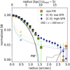 |
Fig. 10. Comparison of our results with a compilation of data at low z in the log(Ṁout)–log(SFR) diagram. The red square (diamond) indicates the average outflow rate for the atomic component obtained from the stacking of the full (high-SFR) sample, while red bars indicate the associated uncertainty (±1σ). The black arrows show our estimate of the total Ṁout (calculated adopting a correction for multi-phase outflows; see text). The orange (cyan) dashed line indicates the best fits for single-phase (three-phases, i.e., molecular, ionised, and atomic) Ṁout observations in local star-forming galaxies, while the magenta dashed line represents the best fit from observation of local AGNs (from Fluetsch et al. 2019). Filled colored regions indicate the 2σ dispersion around the best fits. The green points show the distribution of a sample of local starbursts (Heckman et al. 2015). The blue solid line indicates the 1:1 relation (η = 1). |
This suggests that star-formation feedback, when compared to AGN feedback, is a less efficient mechanism for rapid quenching of normal galaxies in the early Universe. While possibly contributing to the regulation of star formation as in local galaxies (see e.g., Rodríguez Montero et al. 2019), it is likely not the dominant factor needed to explain the observed population of passive galaxies at z ∼ 2 − 3 (e.g., Merlin et al. 2018; Santini et al. 2019; Valentino et al. 2019).
4.2. Intergalactic and circumgalactic metal enrichment
It is still not clear whether or not star formation-driven outflows can actually escape the DM halos and therefore effectively remove the fuel for future star formation. On the one hand, the sensitivity of currently available data (even in the deepest integrations with ALMA, tracing both atomic and molecular FIR lines) is far from being sufficient at revealing the spatial extension of the star-formation-driven winds around individual high-z main sequence galaxies on scales comparable with their virial radii. On the other hand, while the stacking of ALPINE-like large samples can provide significantly improved sensitivity, the randomness of wind directions and geometries strongly challenges the detection of spatially extended outflowing gas (as seen in Sect. 3.4, where the high-velocity [C II] flux is more compact than the core component).
Another way to figure out the fate of the outflows is to compare their typical velocities, voutf, with the escape velocities, vesc, of the DM halos. We estimate vesc of the DM halos hosting the galaxies in our sample, using the formula:
 (6)
(6)
where rDM is the virial radius and MDM is the mass of the halo. We calculate rDM using the commonly adopted hypothesis of virialized halos (see e.g., Huang et al. 2017):
![Mathematical equation: $$ \begin{aligned} r_{\rm DM} = \left[\dfrac{3\;M_{\rm DM}}{4\,\pi \,200\,\rho _{\rm crit}(z)}\right]^{1/3}, \end{aligned} $$](/articles/aa/full_html/2020/01/aa36872-19/aa36872-19-eq23.gif) (7)
(7)
where ρcrit(z) is the critical density of the Universe at redshift z and MDM was estimated using empirically calibrated stellar mass-halo mass (SMHM) relations (see e.g., Behroozi et al. 2013, 2019; Durkalec et al. 2015).
Galaxies in the high-SFR group of our sample, where (as discussed in Sect. 3) the signatures of atomic star-formation-driven outflows are unequivocal, have stellar masses in the range M⋆ = 1010 − 1011.2 M⊙. Those stellar masses, according to the SMHM relation by Behroozi et al. (2019), correspond to DM halos masses in the range MDM ∼ 7 × 10¹¹ − 5 × 10¹² M⊙ and virial radii of rDM ∼ 40 − 100 kpc (Eq. (7)). Therefore, using Eq. (6), we find typical escapes velocities of vesc ∼ 400 − 800 km s−1. These values of vesc, compared with the outflow velocities (vout ≲ 500 km s−1) found in our stacked [C II] spectrum, suggest that a fraction of gas accelerated by star-formation-driven outflows may escape the halo only in less massive galaxies (and possibly contribute to the IGM enrichment, as expected by models; e.g., Oppenheimer et al. 2010; Pallottini et al. 2014; Muratov et al. 2015), while this is unlikely to happen for the more massive galaxies. The outflowing gas that cannot escape the halo would instead be trapped in the CGM and eventually virialize after mixing with both the quiescent and the inflowing primordial gas, producing the large reservoir of enriched circumgalactic gas that we observe in [C II] on scales of ∼30 kpc (see Sect. 3.4; see also a discussion in Fujimoto et al. 2019). Altogether these results confirm the expectations of cosmological simulations (see e.g., Somerville & Davé 2015; Hopkins et al. 2014; Hayward & Hopkins 2017) that the baryon cycle and the enriched gas exchanges with the CGM are at work in normal galaxies already in the early Universe.
5. Conclusions
Here we present the stacking analysis of the [C II] emission detected by ALMA in 50 main sequence star-forming galaxies at 4 < z < 6 (see information on the sample in Sects. 2 and 3.1.2) drawn from the ALPINE survey (Le Fèvre et al. 2019a; Béthermin et al., in prep.; Faisst et al. 2019). The combination of (i) a large statistical sample and (ii) a wealth of ancillary multi-wavelength photometry (from UV to FIR) provided by ALPINE sets the ideal conditions to progress in studying the efficiency of star-formation-driven feedback and circumgalactic enrichment at early epochs. Our main findings can be summarized as follows.
-
To check whether the [C II] line profiles of our galaxies can be sufficiently well described by a single-Gaussian model, we performed a variance-weighted stacking analysis of the [C II] residuals, computed by subtracting a single-component Gaussian fit to each [C II] spectrum (see Sect. 3.2). We observe typical deviations from a single-component Gaussian model, consisting of flux excesses (with peaks at > 4σ) in the high-velocity tails of the stacked residuals, at |v|≲500 km s−1 (Figs. 2 and 3b), in line with previous similar studies carried out on smaller samples (see Gallerani et al. 2018).
-
We performed a variance-weighted stacking of the [C II] spectra (see Sect. 3.3) and find that the stacked [C II] profile of normal star-forming galaxies in our sample is characterized by typical signatures of outflows in its high-velocity tails. In particular, we detect broad wings at velocities of a few hundred kilometers per second (Fig. 5), and find that the average [C II] spectrum can be accurately described by a two-component Gaussian fit (analogous to observations of QSOs; e.g., Maiolino et al. 2012; Cicone et al. 2015; Bischetti et al. 2019), resulting in a combination of a narrow component (FWHM ∼ 230 km s−1) and a relatively less prominent broad component (FWHM ∼ 530 km s−1).
-
We repeated the [C II] residuals and spectra stacking dividing our sample into two equally populated SFR-defined bins, using SFRmed = 25 M⊙ yr−1 as a threshold. We find that both (i) the significance of deviation from a single-component Gaussian model in the combined residuals (Fig. 3) and (ii) the significance of the broad wings in the high-velocity tails of the stacked [C II] spectrum (Fig. 6) increase (decrease) when stacking the subsample of high (low)-SFR galaxies, confirming the star-formation-driven nature of these features. In particular, the stacked [C II] spectrum of high-SFR galaxies shows a broad component with a FWHM of ∼700 km s−1.
-
We constrain the efficiency of star-formation-driven outflows at early epochs estimating the resulting mass-outflow rates (see Sect. 4). We find values roughly comparable with the SFRs (Ṁout ≲ 30 M⊙ yr−1), yielding a mass loading factor lower than (or consistent with) unity (ηatom ≲ 1), similarly to what is found in local, normal star-forming galaxies (Fig. 10; see e.g., Cicone et al. 2016; Fluetsch et al. 2019). Even when considering a contribution to the outflow from multiple gas phases, the estimated mass loading factor (ηtot ∼ 1 − 3) is still below the η observed in AGNs, suggesting that stellar feedback may play a lesser role in quenching galaxies at z > 4 and producing passive galaxies by z ∼ 2 − 3.
-
To better characterize the outflow properties and explore morphologies and spatial extensions of both the core and the high-velocity wings of the [C II] emission, we performed a stacking analysis of the datacubes (see Sect. 3.4). We find that the combined [C II] core emission (|v|< 200 km s−1) of galaxies in the high-SFR subsample extends over physical sizes of ∼30 kpc (diameter scale), well beyond the stacked FIR continuum and the [C II] core emission of lower-SFR galaxies (Fig. 9). The detection of such extended metal-enriched gas, likely tracing circumgalactic gas enriched by past outflows, corroborates previous, similar studies (see Fujimoto et al. 2019; see also Fujimoto et al., in prep.), confirming that the baryon cycle, metal circulation, and gas mixing in the CGM are at work in normal star-forming galaxies in the early Universe.
Following the commonly adopted nomenclature in the literature, we use normal when referring to galaxies on the star-forming Main Sequence (e.g., Brinchmann et al. 2004; Noeske et al. 2007; Daddi et al. 2010; Rodighiero et al. 2011; Speagle et al. 2014).
Velocity-integrated [C II] maps were created in an iterative way, allowing for (i) slight (astrometry-corrected) spatial offsets (< 1″) between the [C II] and rest-frame UV centroids, and (ii) spectral shifts between [C II] line and expected frequencies from UV spectra (see Béthermin et al., in prep., for details).
For the sake of clarity we repeated our analysis leaving the phase centers as common spatial reference points, and the results of cube-stacking are identical within the errors. The lack of evident deviation is due to the fact that only a small fraction (< 10%) of our sample is affected by small offsets (< 1″) between [C II] and rest-frame UV (see a discussion in a similar analysis by Fujimoto et al. 2019).
We estimate a limit of ≲1.5 M⊙ yr−1 on their SFR, based on the absolute UV magnitude limit of our sample.
We note that since the spectra were spectrally centered and aligned at z[C II] (as discussed in Sect. 3.1.1), the center velocity is by definition 0 km s−1.
These weak residuals are consist with the output of a single-Gaussian fit of a curve which is better described by the combination of a narrow and a broad Gaussian components (see Sect. 3.3). Indeed, in this case, a single-Gaussian fit would underestimate the center and overestimate the low-velocity flux in order to get some amplitude out into the high-velocity wings.
Here and in the following, the reported FWHM values are deconvolved for the intrinsic spectral resolution of the stacked spectra (25 km s−1).
The stacked synthesized beam of our observations has a major axis FWHM of 0.98″, a minor axis FWHM of 0.89″, and a position angle of −30 deg.
We calculated beam-deconvolved sizes by fitting a 2D Gaussian model and subtracting in quadrature the major and minor axis FWHM of our stacked synthesized beam.
We estimated the Poissonian noise level by dividing the rms of the normalized [C II]-flux (or continuum) images by the square root of each annulus area.
Acknowledgments
The authors would like to thank the anonymous referee for the useful suggestions. M.G. would like to thank Andrea Ferrara, Simona Gallerani, Andrea Pallottini, Stefano Carniani, Jorryt Matthee, Emanuele Daddi, Andreas Schruba and Roberto Decarli for helpful discussions. G.C.J. and R.M. acknowledge ERC Advanced Grant 695671 “QUENCH” and support by the Science and Technology Facilities Council (STFC). M.B. acknowledges FONDECYT regular grant 1170618. E. I. acknowledges partial support? from FONDECYT through grant N° 1171710. F.L., C.G., F.P. and M.T. acknowledge the support from a grant PRIN MIUR 2017. L.V. acknowledges funding from the European Union’s Horizon 2020 research and innovation program under the Marie Skłodowska-Curie Grant agreement No. 746119. S.T. acknowledges support from the ERC Consolidator Grant funding scheme (project Con-TExT, grant No. 648179). The Cosmic Dawn Center is funded by the Danish National Research Foundation under grant No. 140. R.C. acknowledges financial support from CONICYT Doctorado Nacional N° 21161487 and CONICYT PIA ACT172033. J.D.S is supported by the JSPS KAKENHI Grant Number *JP18H04346*, and the World Premier International Research Center Initiative (WPI Initiative), MEXT, Japan. This paper is based on data obtained with the ALMA Observatory, under Large Program 2017.1.00428.L. ALMA is a partnership of ESO (representing its member states), NSF (USA) and NINS (Japan), together with NRC (Canada), MOST and ASIAA (Taiwan), and KASI (Republic of Korea), in cooperation with the Republic of Chile. The Joint ALMA Observatory is operated by ESO, AUI/NRAO and NAOJ. This program receives financial support from the French CNRS-INSU Programme National Cosmologie et Galaxies.
References
- Arnouts, S., Cristiani, S., Moscardini, L., et al. 1999, MNRAS, 310, 540 [NASA ADS] [CrossRef] [Google Scholar]
- Arribas, S., Colina, L., Bellocchi, E., Maiolino, R., & Villar-Martín, M. 2014, A&A, 568, A14 [NASA ADS] [CrossRef] [EDP Sciences] [Google Scholar]
- Baldwin, J. A., Phillips, M. M., & Terlevich, R. 1981, PASP, 93, 5 [NASA ADS] [CrossRef] [EDP Sciences] [Google Scholar]
- Begeman, K. G. 1989, A&A, 223, 47 [NASA ADS] [Google Scholar]
- Behrens, C., Pallottini, A., Ferrara, A., Gallerani, S., & Vallini, L. 2019, MNRAS, 486, 2197 [NASA ADS] [CrossRef] [Google Scholar]
- Behroozi, P. S., Wechsler, R. H., & Conroy, C. 2013, ApJ, 770, 57 [NASA ADS] [CrossRef] [Google Scholar]
- Behroozi, P., Wechsler, R. H., Hearin, A. P., & Conroy, C. 2019, MNRAS, 488, 3143 [NASA ADS] [CrossRef] [Google Scholar]
- Benson, A. J., Bower, R. G., Frenk, C. S., et al. 2003, ApJ, 599, 38 [NASA ADS] [CrossRef] [Google Scholar]
- Bigiel, F., Leroy, A. K., Walter, F., et al. 2011, ApJ, 730, L13 [NASA ADS] [CrossRef] [Google Scholar]
- Bischetti, M., Maiolino, R., Carniani, S., et al. 2019, A&A, 630, A59 [NASA ADS] [CrossRef] [EDP Sciences] [Google Scholar]
- Bower, R. G., Benson, A. J., Malbon, R., et al. 2006, MNRAS, 370, 645 [NASA ADS] [CrossRef] [Google Scholar]
- Bradač, M., Garcia-Appadoo, D., Huang, K.-H., et al. 2017, ApJ, 836, L2 [NASA ADS] [CrossRef] [Google Scholar]
- Brinchmann, J., Charlot, S., White, S. D. M., et al. 2004, MNRAS, 351, 1151 [NASA ADS] [CrossRef] [Google Scholar]
- Bruzual, G., & Charlot, S. 2003, MNRAS, 344, 1000 [NASA ADS] [CrossRef] [Google Scholar]
- Capak, P. L., Carilli, C., Jones, G., et al. 2015, Nature, 522, 455 [NASA ADS] [CrossRef] [Google Scholar]
- Carniani, S., Marconi, A., Biggs, A., et al. 2013, A&A, 559, A29 [NASA ADS] [CrossRef] [EDP Sciences] [Google Scholar]
- Carniani, S., Maiolino, R., Amorin, R., et al. 2018, MNRAS, 478, 1170 [NASA ADS] [CrossRef] [Google Scholar]
- Cattaneo, A., Faber, S. M., Binney, J., et al. 2009, Nature, 460, 213 [NASA ADS] [CrossRef] [PubMed] [Google Scholar]
- Chabrier, G. 2003, PASP, 115, 763 [NASA ADS] [CrossRef] [Google Scholar]
- Chisholm, J., Tremonti, C. A., Leitherer, C., et al. 2015, ApJ, 811, 149 [NASA ADS] [CrossRef] [Google Scholar]
- Chisholm, J., Tremonti Christy, A., Leitherer, C., & Chen, Y. 2016, MNRAS, 463, 541 [NASA ADS] [CrossRef] [Google Scholar]
- Chisholm, J., Tremonti, C. A., Leitherer, C., & Chen, Y. 2017, MNRAS, 469, 4831 [NASA ADS] [CrossRef] [Google Scholar]
- Cicone, C., Maiolino, R., Gallerani, S., et al. 2015, A&A, 574, A14 [NASA ADS] [CrossRef] [EDP Sciences] [Google Scholar]
- Cicone, C., Maiolino, R., & Marconi, A. 2016, A&A, 588, A41 [NASA ADS] [CrossRef] [EDP Sciences] [Google Scholar]
- Cormier, D., Lebouteiller, V., Madden, S. C., et al. 2012, A&A, 548, A20 [NASA ADS] [CrossRef] [EDP Sciences] [Google Scholar]
- Daddi, E., Bournaud, F., Walter, F., et al. 2010, ApJ, 713, 686 [NASA ADS] [CrossRef] [Google Scholar]
- de Blok, W. J. G., Walter, F., Smith, J. D. T., et al. 2016, AJ, 152, 51 [NASA ADS] [CrossRef] [Google Scholar]
- De Breuck, C., Williams, R. J., Swinbank, M., et al. 2014, A&A, 565, A59 [NASA ADS] [CrossRef] [EDP Sciences] [Google Scholar]
- Decarli, R., Walter, F., Venemans, B. P., et al. 2018, ApJ, 854, 97 [NASA ADS] [CrossRef] [Google Scholar]
- Dekel, A., & Silk, J. 1986, ApJ, 303, 39 [NASA ADS] [CrossRef] [Google Scholar]
- Di Teodoro, E. M., & Fraternali, F. 2015, MNRAS, 451, 3021 [NASA ADS] [CrossRef] [Google Scholar]
- Durkalec, A., Le Fèvre, O., de la Torre, S., et al. 2015, A&A, 576, L7 [NASA ADS] [CrossRef] [EDP Sciences] [Google Scholar]
- Erb, D. K. 2015, Nature, 523, 169 [NASA ADS] [CrossRef] [Google Scholar]
- Fabian, A. C. 2012, ARA&A, 50, 455 [NASA ADS] [CrossRef] [Google Scholar]
- Faisst, A., Bethermin, M., Capak, P., et al. 2019, ArXiv e-prints [arXiv:1901.01268] [Google Scholar]
- Ferrara, A., Vallini, L., Pallottini, A., et al. 2019, MNRAS, 489, 1 [NASA ADS] [CrossRef] [Google Scholar]
- Feruglio, C., Fiore, F., Carniani, S., et al. 2018, A&A, 619, A39 [NASA ADS] [CrossRef] [EDP Sciences] [Google Scholar]
- Fiore, F., Feruglio, C., Shankar, F., et al. 2017, A&A, 601, A143 [NASA ADS] [CrossRef] [EDP Sciences] [Google Scholar]
- Fluetsch, A., Maiolino, R., Carniani, S., et al. 2019, MNRAS, 483, 4586 [NASA ADS] [Google Scholar]
- Fruchter, A. S., & Hook, R. N. 2002, PASP, 114, 144 [NASA ADS] [CrossRef] [Google Scholar]
- Fujimoto, S., Ouchi, M., Ferrara, A., et al. 2019, ApJ, 887, 107 [NASA ADS] [CrossRef] [Google Scholar]
- Gallerani, S., Pallottini, A., Feruglio, C., et al. 2018, MNRAS, 473, 1909 [NASA ADS] [CrossRef] [Google Scholar]
- García-Burillo, S., Combes, F., Usero, A., et al. 2015, A&A, 580, A35 [NASA ADS] [CrossRef] [EDP Sciences] [Google Scholar]
- Hailey-Dunsheath, S., Nikola, T., Stacey, G. J., et al. 2010, ApJ, 714, L162 [NASA ADS] [CrossRef] [Google Scholar]
- Hashimoto, T., Laporte, N., Mawatari, K., et al. 2018, Nature, 557, 392 [NASA ADS] [CrossRef] [Google Scholar]
- Hasinger, G., Capak, P., Salvato, M., et al. 2018, ApJ, 858, 77 [NASA ADS] [CrossRef] [Google Scholar]
- Hayward, C. C., & Hopkins, P. F. 2017, MNRAS, 465, 1682 [Google Scholar]
- Heckman, T. M., & Thompson, T. A. 2017, ArXiv e-prints [arXiv:1701.09062] [Google Scholar]
- Heckman, T. M., Armus, L., & Miley, G. K. 1990, ApJS, 74, 833 [NASA ADS] [CrossRef] [Google Scholar]
- Heckman, T. M., Alexandroff, R. M., Borthakur, S., Overzier, R., & Leitherer, C. 2015, ApJ, 809, 147 [NASA ADS] [CrossRef] [Google Scholar]
- Hollenbach, D. J., & Tielens, A. G. G. M. 1999, Rev. Mod. Phys., 71, 173 [Google Scholar]
- Hopkins, P. F., Quataert, E., & Murray, N. 2012, MNRAS, 421, 3522 [Google Scholar]
- Hopkins, P. F., Kereš, D., Oñorbe, J., et al. 2014, MNRAS, 445, 581 [NASA ADS] [CrossRef] [Google Scholar]
- Hopkins, P. F., Torrey, P., Faucher-Giguère, C.-A., Quataert, E., & Murray, N. 2016, MNRAS, 458, 816 [NASA ADS] [CrossRef] [Google Scholar]
- Huang, K.-H., Fall, S. M., Ferguson, H. C., et al. 2017, ApJ, 838, 6 [NASA ADS] [CrossRef] [Google Scholar]
- Ilbert, O., Arnouts, S., McCracken, H. J., et al. 2006, A&A, 457, 841 [NASA ADS] [CrossRef] [EDP Sciences] [Google Scholar]
- Inoue, A. K., Tamura, Y., Matsuo, H., et al. 2016, Science, 352, 1559 [NASA ADS] [CrossRef] [Google Scholar]
- Janssen, A. W., Christopher, N., Sturm, E., et al. 2016, ApJ, 822, 43 [NASA ADS] [Google Scholar]
- Jones, G. C., Carilli, C. L., Shao, Y., et al. 2017, ApJ, 850, 180 [NASA ADS] [CrossRef] [Google Scholar]
- Kaufman, M. J., Wolfire, M. G., Hollenbach, D. J., & Luhman, M. L. 1999, ApJ, 527, 795 [NASA ADS] [CrossRef] [Google Scholar]
- Kaufman, M. J., Wolfire, M. G., & Hollenbach, D. J. 2006, ApJ, 644, 283 [NASA ADS] [CrossRef] [Google Scholar]
- Kennicutt, Jr., R. C. 1998, ARA&A, 36, 189 [Google Scholar]
- Kohandel, M., Pallottini, A., Ferrara, A., et al. 2019, MNRAS, 487, 3007 [NASA ADS] [CrossRef] [Google Scholar]
- Krumholz, M. R., & McKee, C. F. 2005, ApJ, 630, 250 [NASA ADS] [CrossRef] [Google Scholar]
- Lagache, G., Cousin, M., & Chatzikos, M. 2018, A&A, 609, A130 [NASA ADS] [CrossRef] [EDP Sciences] [Google Scholar]
- Laigle, C., McCracken, H. J., Ilbert, O., et al. 2016, ApJS, 224, 24 [NASA ADS] [CrossRef] [Google Scholar]
- Le Fèvre, O., Tasca, L. A. M., Cassata, P., et al. 2015, A&A, 576, A79 [NASA ADS] [CrossRef] [EDP Sciences] [Google Scholar]
- Le Fèvre, O., Béthermin, M., Faisst, A., et al. 2019a, A&A, submitted [arXiv:1910.09517] [Google Scholar]
- Le Fèvre, O., Lemaux, B. C., Nakajima, K., et al. 2019b, A&A, 625, A51 [NASA ADS] [CrossRef] [EDP Sciences] [Google Scholar]
- Leroy, A. K., Walter, F., Brinks, E., et al. 2008, AJ, 136, 2782 [NASA ADS] [CrossRef] [Google Scholar]
- Leroy, A. K., Walter, F., Sandstrom, K., et al. 2013, AJ, 146, 19 [NASA ADS] [CrossRef] [Google Scholar]
- Mac Low, M.-M., & Ferrara, A. 1999, ApJ, 513, 142 [NASA ADS] [CrossRef] [Google Scholar]
- Maiolino, R., Gallerani, S., Neri, R., et al. 2012, MNRAS, 425, L66 [NASA ADS] [CrossRef] [Google Scholar]
- Maiolino, R., Carniani, S., Fontana, A., et al. 2015, MNRAS, 452, 54 [NASA ADS] [CrossRef] [Google Scholar]
- Matthee, J., Sobral, D., Boogaard, L. A., et al. 2019, ApJ, 881, 124 [NASA ADS] [CrossRef] [Google Scholar]
- McMullin, J. P., Waters, B., Schiebel, D., Young, W., & Golap, K. 2007, in Astronomical Data Analysis Software and Systems XVI, eds. R. A. Shaw, F. Hill, & D. J. Bell, ASP Conf. Ser., 376, 127 [Google Scholar]
- Merlin, E., Fontana, A., Castellano, M., et al. 2018, MNRAS, 473, 2098 [NASA ADS] [CrossRef] [Google Scholar]
- Muratov, A. L., Kereš, D., Faucher-Giguère, C.-A., et al. 2015, MNRAS, 454, 2691 [NASA ADS] [CrossRef] [Google Scholar]
- Nakajima, K., Schaerer, D., Le Fèvre, O., et al. 2018, A&A, 612, A94 [NASA ADS] [CrossRef] [EDP Sciences] [Google Scholar]
- Noeske, K. G., Weiner, B. J., Faber, S. M., et al. 2007, ApJ, 660, L43 [Google Scholar]
- Oppenheimer, B. D., & Davé, R. 2006, MNRAS, 373, 1265 [NASA ADS] [CrossRef] [Google Scholar]
- Oppenheimer, B. D., Davé, R., Kereš, D., et al. 2010, MNRAS, 406, 2325 [NASA ADS] [CrossRef] [Google Scholar]
- Pallottini, A., Gallerani, S., & Ferrara, A. 2014, MNRAS, 444, L105 [NASA ADS] [CrossRef] [Google Scholar]
- Pallottini, A., Ferrara, A., Decataldo, D., et al. 2019, MNRAS, 487, 1689 [NASA ADS] [CrossRef] [Google Scholar]
- Riechers, D. A., Carilli, C. L., Capak, P. L., et al. 2014, ApJ, 796, 84 [NASA ADS] [CrossRef] [Google Scholar]
- Rodighiero, G., Daddi, E., Baronchelli, I., et al. 2011, ApJ, 739, L40 [NASA ADS] [CrossRef] [Google Scholar]
- Rodríguez del Pino, B., Arribas, S., Piqueras López, J., Villar-Martín, M., & Colina, L. 2019, MNRAS, 486, 344 [NASA ADS] [CrossRef] [Google Scholar]
- Rodríguez Montero, F., Davé, R., Wild, V., Anglés-Alcázar, D., & Narayanan, D. 2019, MNRAS, 490, 2139 [NASA ADS] [CrossRef] [Google Scholar]
- Rubin, K. H. R., Weiner, B. J., Koo, D. C., et al. 2010, ApJ, 719, 1503 [NASA ADS] [CrossRef] [Google Scholar]
- Rubin, K. H. R., Prochaska, J. X., Koo, D. C., et al. 2014, ApJ, 794, 156 [NASA ADS] [CrossRef] [Google Scholar]
- Rupke, D. 2018, Galaxies, 6, 138 [NASA ADS] [CrossRef] [Google Scholar]
- Rupke, D. S., Veilleux, S., & Sanders, D. B. 2005, ApJS, 160, 115 [NASA ADS] [CrossRef] [Google Scholar]
- Santini, P., Merlin, E., Fontana, A., et al. 2019, MNRAS, 486, 560 [NASA ADS] [CrossRef] [Google Scholar]
- Savage, B. D., & Sembach, K. R. 1996, ARA&A, 34, 279 [NASA ADS] [CrossRef] [Google Scholar]
- Shapley, A. E., Steidel, C. C., Pettini, M., & Adelberger, K. L. 2003, ApJ, 588, 65 [NASA ADS] [CrossRef] [Google Scholar]
- Silk, J., & Mamon, G. A. 2012, Res. Astron. Astrophys., 12, 917 [NASA ADS] [CrossRef] [Google Scholar]
- Smit, R., Bouwens, R. J., Carniani, S., et al. 2018, Nature, 553, 178 [NASA ADS] [CrossRef] [Google Scholar]
- Somerville, R. S., & Davé, R. 2015, ARA&A, 53, 51 [NASA ADS] [CrossRef] [EDP Sciences] [Google Scholar]
- Speagle, J. S., Steinhardt, C. L., Capak, P. L., & Silverman, J. D. 2014, ApJS, 214, 15 [NASA ADS] [CrossRef] [Google Scholar]
- Stacey, G. J., Geis, N., Genzel, R., et al. 1991, ApJ, 373, 423 [NASA ADS] [CrossRef] [Google Scholar]
- Stacey, G. J., Hailey-Dunsheath, S., Ferkinhoff, C., et al. 2010, ApJ, 724, 957 [NASA ADS] [CrossRef] [Google Scholar]
- Stanley, F., Jolly, J. B., König, S., & Knudsen, K. K. 2019, A&A, 631, A78 [NASA ADS] [CrossRef] [EDP Sciences] [Google Scholar]
- Steidel, C. C., Shapley, A. E., Pettini, M., et al. 2004, ApJ, 604, 534 [NASA ADS] [CrossRef] [Google Scholar]
- Steidel, C. C., Erb, D. K., Shapley, A. E., et al. 2010, ApJ, 717, 289 [NASA ADS] [CrossRef] [Google Scholar]
- Sugahara, Y., Ouchi, M., Lin, L., et al. 2017, ApJ, 850, 51 [NASA ADS] [CrossRef] [Google Scholar]
- Sugahara, Y., Ouchi, M., Harikane, Y., et al. 2019, ApJ, 886, 29 [NASA ADS] [CrossRef] [Google Scholar]
- Talia, M., Mignoli, M., Cimatti, A., et al. 2012, A&A, 539, A61 [NASA ADS] [CrossRef] [EDP Sciences] [Google Scholar]
- Talia, M., Brusa, M., Cimatti, A., et al. 2017, MNRAS, 471, 4527 [NASA ADS] [CrossRef] [Google Scholar]
- Talia, M., Pozzi, F., Vallini, L., et al. 2018, MNRAS, 476, 3956 [NASA ADS] [CrossRef] [EDP Sciences] [Google Scholar]
- Tasca, L. A. M., Le Fèvre, O., Ribeiro, B., et al. 2017, A&A, 600, A110 [NASA ADS] [CrossRef] [EDP Sciences] [Google Scholar]
- Valentino, F., Tanaka, M., Davidzon, I., et al. 2019, ApJ, submitted [arXiv:1909.10540] [Google Scholar]
- Vallini, L., Gallerani, S., Ferrara, A., Pallottini, A., & Yue, B. 2015, ApJ, 813, 36 [NASA ADS] [CrossRef] [Google Scholar]
- Vallini, L., Ferrara, A., Pallottini, A., & Gallerani, S. 2017, MNRAS, 467, 1300 [NASA ADS] [Google Scholar]
- Veilleux, S., Cecil, G., & Bland-Hawthorn, J. 2005, ARA&A, 43, 769 [Google Scholar]
- Wagg, J., Wiklind, T., Carilli, C. L., et al. 2012, ApJ, 752, L30 [NASA ADS] [CrossRef] [Google Scholar]
- Wolfire, M. G., McKee, C. F., Hollenbach, D., & Tielens, A. G. G. M. 2003, ApJ, 587, 278 [NASA ADS] [CrossRef] [Google Scholar]
- Woosley, S. E., Heger, A., & Weaver, T. A. 2002, Rev. Mod. Phys., 74, 1015 [NASA ADS] [CrossRef] [Google Scholar]
All Tables
Median SFRs of full and high-SFR (sub)samples are summarized, along with the FWHMs of both narrow and broad Gaussian components.
All Figures
|
Fig. 1. Redshift (a), SFR (b), and M⋆ (c) distributions of galaxies in the ALPINE survey (orange) and galaxies in our final sample (blue), drawn from ALPINE and used in this work (see Sect. 3.1.2). For comparison, in panels b and c we show the SFR and M⋆ distributions of all COSMOS galaxies with photometric redshift in the ALPINE range z = [4.4 − 5.8] (from Laigle et al. 2016). The gap in the redshift distribution is due to the original ALPINE sample selection, tailored to avoid a prominent atmospheric absorption at ∼325 GHz in ALMA band 7. The black dashed lines in panels b and c represent the median SFR and Mstar of galaxies in our ALPINE-drawn sample. |
| In the text | |
|
Fig. 2. Top: histogram containing the number of objects per channel contributing to the stacked flux. Central lower panel: variance-weighted stacked [C II] residuals from a single-Gaussian fit in spectral bins of 25 km s−1 (75 km s−1). The green solid lines at ±800 km s−1 enclose the velocity range excluded for the estimation of spectral noise, while the blue dashed lines represent the spectral rms at ±1σ. Channels in violet represent the channels in the velocity range enclosed by the outermost peaks at ≥3σ in the 75 km s−1-binned stacked residuals. This helps in visualizing the velocity interval affected by flux excesses. |
| In the text | |
|
Fig. 3. Same description as in Fig. 2. Here the stacked residuals are shown for the low-SFR (a), and the high-SFR (b) groups, respectively. While the stacked residuals are consistent with the noise in the low-SFR subsample, significant (> 4σ) peaks of flux excess are detected for high-SFR galaxies. |
| In the text | |
|
Fig. 4. Similar to the central panel of Fig. 3b, the 25 km s−1-binned stacked [C II] residuals of the high-SFR group are shown. However, here, for the five rotators in the subsample, Ri, k (see Eq. (1)) is calculated by subtracting a kinematic model to the observed spectra. We color in green the channels where the residuals left by the tilted-ring fit are non-null, specifically in the velocity range v ∼ [ − 225 : + 275] km s−1, marked by the gray shaded region. |
| In the text | |
|
Fig. 5. a: variance-weighted stacked [C II] spectrum of all galaxies in our sample is shown, in velocity bins of 25 km s−1. The orange (blue) line shows the single-Gaussian (two-Gaussian) best-fit. The red and the green line represent the narrow and broad components of the two-Gaussian model, respectively. A zoom of the velocity range [ − 600 : + 600] km s−1 is shown in the inset. A histogram containing the number of objects per channel contributing to the stacking is shown in the top panel. b: residuals from the single-Gaussian (two-Gaussian) best-fit are shown in red (blue), in velocity bins of 50 km s−1. |
| In the text | |
|
Fig. 6. Same description as in Fig. 5. In this case the stacked [C II] spectrum and corresponding residuals from a single- and two-Gaussian best-fits are shown for the low-SFR (a), and the high-SFR (b) subsamples, individually. |
| In the text | |
|
Fig. 7. Distribution of the FWHM of narrow (red histograms) and broad (green histograms) components obtained with a bootstrap analysis for the full sample (a) and the high-SFR group (b). The dashed lines represent the median values of the distribution. |
| In the text | |
|
Fig. 8. Velocity-integrated [C II] flux maps (central 8″ × 8″ regions) are shown in different velocity ranges, from the combined cubes obtained by stacking (a) the full sample, (b) the low-SFR, and (c) the high-SFR groups. Left and right panels: representative of the high-velocity tails of the [C II] emission ([ − 600 : − 200] and [ + 200 : + 600] km s−1, respectively), while maps in the central panels trace the [C II] core ([ − 200 : + 200] km s−1). Significance levels of the black contours are reported below the panels of (a). The average synthesized beam is shown in the lower-left corners, while a reference size-scale of 15 kpc is reported at the bottom of each panel. The center of each panel is marked with a white cross. |
| In the text | |
|
Fig. 9. Circularly averaged radial profiles computed in concentric 0.3″-binned annuli are shown for (i) the stacked PSF of our ALMA observations (black solid line for galaxies in our sample, and black dashed line for ALPINE continuum-detected galaxies), (ii) the stacked FIR continuum of 23 ALPINE continuum-detected galaxies (mostly belonging to the high-SFR group, see text; orange squares), and (iii) the stacked maps of [C II] cores ([ − 200 : + 200] km s−1) for galaxies in the low-SFR (green squares) and high-SFR (blue square) groups. Error bars are indicative of the ±1σ dispersion of fluxes in each annulus, while the thin dashed lines represent the Poissonian noise associated with the radial profiles10. |
| In the text | |
|
Fig. 10. Comparison of our results with a compilation of data at low z in the log(Ṁout)–log(SFR) diagram. The red square (diamond) indicates the average outflow rate for the atomic component obtained from the stacking of the full (high-SFR) sample, while red bars indicate the associated uncertainty (±1σ). The black arrows show our estimate of the total Ṁout (calculated adopting a correction for multi-phase outflows; see text). The orange (cyan) dashed line indicates the best fits for single-phase (three-phases, i.e., molecular, ionised, and atomic) Ṁout observations in local star-forming galaxies, while the magenta dashed line represents the best fit from observation of local AGNs (from Fluetsch et al. 2019). Filled colored regions indicate the 2σ dispersion around the best fits. The green points show the distribution of a sample of local starbursts (Heckman et al. 2015). The blue solid line indicates the 1:1 relation (η = 1). |
| In the text | |
Current usage metrics show cumulative count of Article Views (full-text article views including HTML views, PDF and ePub downloads, according to the available data) and Abstracts Views on Vision4Press platform.
Data correspond to usage on the plateform after 2015. The current usage metrics is available 48-96 hours after online publication and is updated daily on week days.
Initial download of the metrics may take a while.