| Issue |
A&A
Volume 633, January 2020
|
|
|---|---|---|
| Article Number | A44 | |
| Number of page(s) | 16 | |
| Section | Planets and planetary systems | |
| DOI | https://doi.org/10.1051/0004-6361/201936038 | |
| Published online | 10 January 2020 | |
A HARPS RV search for planets around young nearby stars★
1
Univ. Grenoble Alpes, CNRS, IPAG,
38000
Grenoble,
France
e-mail: This email address is being protected from spambots. You need JavaScript enabled to view it.
2
Max Planck Institute for Astronomy,
Königstuhl 17,
69117
Heidelberg,
Germany
3
CNRS Lesia (UMR8109) – Observatoire de Paris,
Paris,
France
4
INAF – Osservatorio Astronomico di Padova,
Vicolo dell’Osservatorio 5,
Padova
35122,
Italy
5
INAF – Osservatorio Astrofisico di Catania,
via Santa Sofia, 78
Catania,
Italy
6
European Southern Observatory (ESO), Alonso de Córdova 3107,
Vitacura,
Casilla
19001,
Santiago,
Chile
7
Departamento de Astronomía, Universidad de Chile, Camino al Observatorio,
Cerro Calán,
Santiago,
Chile
8
Oxford Astrophysics, Department of Physics,
Denys Wilkinson Building,
UK
Received:
6
June
2019
Accepted:
14
October
2019
Abstract
Context. Young nearby stars are good candidates in the search for planets with both radial velocity (RV) and direct imaging techniques. This, in turn, allows for the computation of the giant planet occurrence rates at all separations. The RV search around young stars is a challenge as they are generally faster rotators than older stars of similar spectral types and they exhibit signatures of magnetic activity (spots) or pulsation in their RV time series. Specific analyses are necessary to characterize, and possibly correct for, this activity.
Aims. Our aim is to search for planets around young nearby stars and to estimate the giant planet (GP) occurrence rates for periods up to 1000 days.
Methods. We used the HARPS spectrograph on the 3.6 m telescope at La Silla Observatory to observe 89 A−M young (<600 Myr) stars. We used our SAFIR (Spectroscopic data via Analysis of the Fourier Interspectrum Radial velocities) software to compute the RV and other spectroscopic observables. Then, we computed the companion occurrence rates on this sample.
Results. We confirm the binary nature of HD 177171, HD 181321 and HD 186704. We report the detection of a close low mass stellar companion for HIP 36985. No planetary companion was detected. We obtain upper limits on the GP (<13 MJup) and BD (∈ [13;80] MJup) occurrence rates based on 83 young stars for periods less than 1000 days, which are set, 2−2+3 and 1−1+3%.
Key words: techniques: radial velocities / stars: activity / binaries: spectroscopic / planetary systems / starspots / stars: variables: general
A table of the radial velocities is only available at the CDS via anonymous ftp to cdsarc.u-strasbg.fr (130.79.128.5) or via http://cdsarc.u-strasbg.fr/viz-bin/cat/J/A+A/633/A44
© A. Grandjean et al. 2020
 Open Access article, published by EDP Sciences, under the terms of the Creative Commons Attribution License (http://creativecommons.org/licenses/by/4.0), which permits unrestricted use, distribution, and reproduction in any medium, provided the original work is properly cited.
1 Introduction
More than four thousand exoplanets have been confirmed and most of them have been found by transit or radial velocity (RV) techniques1. The latter, although very powerful, is limited by the parent star’s activity (spots, plages, convection, and pulsations). Young stars are generally faster rotators than their older counterparts (Stauffer et al. 2016; Rebull et al. 2016; Gallet & Bouvier 2015). They can also exhibit activity-induced RV jitter with amplitudes up to 1 km s−1 (Lagrange et al. 2013), larger than the planet’s induced signal. False positive detections have been reported around young stars in the past (Huélamo et al. 2008; Figueira et al. 2010; Soto et al. 2015).
We have carried out an RV survey to search for planets around such young stars with the High Accuracy Radial velocity Planet Searcher (HARPS; Mayor et al. 2003) and SOPHIE (Bouchy & Sophie Team 2006) spectrographs with the final aim of coupling RV data with direct imaging (DI) data, which will allow for the computation of detection limits, for each targets at all separations and then to compute occurrences rates for all separations. A feasibility study was carried out by Lagrange et al. (2013) on 26 stars of the survey with HARPS, demonstrating that we can probe for giant planets (1–13 MJup, hereafter GP) with semi-major axis up to 2 au and couple the survey data with direct imaging data. The time baseline of our survey also permits a probe of the hot Jupiter (hereafter HJ) domain around young stars. Although GP formation models predict a formation at a few au (Pollack et al. 1996), migration through disc-planet interaction (Kley & Nelson 2012) or gravitational interaction with a third body can allow the planet to finally orbit close to the star (Teyssandier et al. 2019). HJ are common among exoplanets orbiting older main sequence stars as they represent one detected planet out of five (Wright et al. 2012). While previous RV surveys on small sets of young stars showed no evidence for the presence of young HJ (Esposito et al. 2006; Paulson & Yelda 2006), two HJ around young stars were recently discovered by Donati et al. (2016) and Yu et al. (2017). However, we still need to find out if this kind of object is common at young age or not and we need to compare the migration models with observations in order to constrain the migration timescales.
Here, we report on the results of our large HARPS survey. We describe our survey sample and observations in Sect. 2. In Sect. 3, we focus on GP, brown dwarf (BD), and stellar companions detections. In Sect. 4, we perform a statistical analysis of our sample and compute the close GP and BD occurrence rates around young stars. We conclude our findings in Sect. 5.
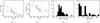 |
Fig. 1 Main physical properties of our sample. (a) Absolute V -magnitude vs. B− V. Each black dot corresponds to one target. The Sun is displayed (red star) for comparison. (b) v sin i vs B− V distribution. (c) Mass histogram (in M⊙). (d) Age histogram. |
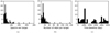 |
Fig. 2 Observation summary. (a) Histogram of the number of spectra per target, excluding HD 216956 (Fomalhaut, 834 spectra) and HD 039060 (β Pic, 5108 spectra). (b) Histogram of the number of nights per target. (c) Histogram of the time baselines. |
2 Description of the survey
2.1 Sample
We selected a sample of 89 stars, chosen to their brightness (V < 10), ages as fund in the literature (<300 Myr for most of them, see Table A.1), and distance (<80 pc) determined from their HIPPARCOS parallaxes (van Leeuwen 2007). These criteria ensure we will get the best detection limits for both the HARPS RV and SPHERE DI surveys at, respectively, short (typically 2− 5 au), and large (further than typically 5 au) separations. Indeed, observing bright stars allow us to obtain spectra with a better signal-to-noise ratio (S/N). Moreover, young planets are still warm from their formation and are then brighter, which lowers the contrast between them and their host stars, while short distances allow for better angular resolutions in direct imaging. Most of the targets are part of the SPHERE GTO The SpHere INfrared survey for Exoplanets (SHINE) survey sample (Chauvin et al. 2017a). Binary stars with an angular separation on the sky that is lower than 2 as were not selected to avoid contamination in the spectra from the companion
Their spectral types range from A0V to M5V (Fig. 1). Their projected rotational velocity (v sin i) range from 0.5 to 300 km s−1 with a median of 11 km s−1, their V-band magnitude are mainly between 4 and 10 with a median of 7.8. Their masses are between 0.6 and 2.74 M⊙ with median of 1.07 M⊙. Our sample includes 26 targets between A0 and F5V(B−V ∈ [−0.05 : 0.52]), 55 between F6 and K5 (B−V ∈ [−0.05 : 0.52]), and 8 between K6 and M5 (B−V ≥ 1.33). Noticeably, our sample includes stars with imaged planetary or substellar companions (among them β Pic, AB Pic, HNPeg, GJ 504, HR 8799, HD 95086, HD 106906 or PZ Tel). We present the main characteristics of our star sample in Fig. 1 and Table A.1.
2.2 Observations
We observed our 89 targets mainly between 2013 and 2016. Some stars were part of previous surveys by Borgniet et al. (2017) and Lagrange et al. (2009a), which allows us to reach a time baseline up to 10 yr. Some stars had already been observed with HARPS before, some since the HARPS commissioning in 2003. Additional observationswere also obtained in October 2017, December 2017, and March 2018.
We use the observing strategy described in Borgniet et al. (2017), which consist of recording two spectra per visit and to observe each target on several consecutive nights to have a good sampling of the short-term jitter. The median time baseline is 1639 days (mean time baseline of 2324 days), with a median number of spectra per target of 25 (52 on average) spaced on a median number of 12 nights (17 on average, Fig. 2). Details can be found in Table A.1.
2.3 Observables
From the HARPS spectra we derived the RV and whenever possible the cross-correlation function (CCF), bisector velocity span (hereafter BVS), and log  with our SAFIR software for Spectroscopic data via Analysis of the Fourier Interspectrum Radial velocities. It builds a reference spectrum from the median of all spectra available on a given star and computes the relative RV in the Fourier plane. The computed RV are then relative to the reference spectrum. The efficiency of this method was proved in the search of companions (Galland et al. 2005a,b). We mainly use the correlation between RV and BVS to determine the main source of RV variability: magnetic activity, pulsations or companions (Lagrange et al. 2009a; Borgniet et al. 2017). We excluded spectra with S/N at 550 nm which was too high (> 380), to avoid saturation or too low (<80), to avoid bad data, as well as spectra with an air mass that was too high (sec z > 3), and spectra that were too different from the reference spectrum of the star (χ2 > 10). For M-type stars, we used a lower limit of 40 in S/N at 550 nm as it is a better compromise for these stars to provide enough spectra to perform our analysis without including bad spectra.
3 Detected companions in the HARPS survey
3.1 Longperiod companions, RV long-term trends, and stellar binaries
In this section we describe the stars for which we identified a GP companion with a period higher than 1000 days, a long-term trend RV signal or a binary signal. When possible, we characterize the companion using the yorbit software that fits RV with a sum of Keplerian or a sum of keplerians plus a drift (Ségransan et al. 2011).
3.1.1 HD 39060
β Pic is an A6V pulsating star that hosts an imaged edge-on debris (Smith & Terrile 1984) and gas disk (Hobbs et al. 1985), and an imaged GP at 9 au (Lagrange et al. 2009b, 2019a). This star presents also exocomets signatures in its spectra (Lagrange-Henri et al. 1988; Beust et al. 1989; Kiefer et al. 2014). β Pic was observed with HARPS since its commissioning in 2003, totalizing more than 6000 spectra with a mean S/N at 550 nm of 273. Until 2008, spectra were taken to study the Ca II absorption lines associated to the falling exocomets. Since 2008, we adopted a specific observation strategy, to properly sample the stellar pulsations and to correct the RV from them, (Lagrange et al. 2012, 2019b). It consisted in observing the star for continuous sequences of 1− 2 h. Longer sequences up to 6h were obtained in 2017−2018. This allowed to detect a new GP companion within the pulsations signal of β Pic. The discovery of this 10 MJup, 1200 days period companion is detailed in Lagrange et al. (2019b).
3.1.2 HD 106906
HD 106906 is a F5V star in the Sco-Cen young association. Bailey et al. (2014) Imaged a giant planet companion at 7.1 as (650 au) in 2014. HARPS data from this survey together with the PIONER interferometer data allowed to detect a close low mass stellar companion to HD 106906 with a period of 10 days, (Lagrange et al. 2015). The presence of the binary could explain the wide orbit of HD 106906b under some circumstances (Rodet et al. 2017).
3.1.3 HD 131399
HD 131399 is member of a complex hierarchical system. HD 131399A forms a binary with the tight binary HD 131399BC. A GP companion was discovered with SPHERE around HD 131399A by Wagner et al. (2016) but is now identified as a background star with similar proper motion (Nielsen et al. 2017). We detected in this survey the presence of a close stellar companion to HD 131399A, with a period of 10 days (0.1 au), and an M sini of 450 MJup (Lagrange et al. 2017).
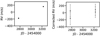 |
Fig. 3 HD 186704 RV long term trend. Left: RV time variations, right: RV corrected from the RV-BVS correlation time variations. |
3.1.4 HD 177171
HD 177 171 (ρ Tel) was reported as a spectroscopic binary by Nordström et al. (2004) and as an astrometric binary by Frankowski & Jorissen (2007) from the HIPPARCOS data. This is confirmed by Lagrange et al. (2013) in the feasibility study of this survey. We measure an amplitude of at least 20 km s−1 in the RV. Our time sampling does not allow for the estimation the period of this stellar companion.
3.1.5 HD 186704A
HD 186704 is a known binary system with a companion at 10 as (Zuckerman et al. 2013). Nidever et al. (2002) report a trend in the RV of 88 ± 8 ms−1 d−1 with a negative curvature based on 4 observationsspaced on 70 days for HD 186704AB. Tremko et al. (2010) observe a change in the RV of 4200 ms−1 in 8682 days on HD 186704A. Finally, Tokovinin (2014) reporte HD 186704A as hosting a spectroscopic binary (SB) companion with a 3990 days period. We observe a trend of 340 ms−1 over a duration of 450 days in the RV of HD 186704A based on 4 spectra. This corresponds to a slope of 0.75 ms−1 d−1. The star present signs of activity, we therefore corrected the RV using the RV-BVS correlation using Melo et al. (2007) method (see Appendix B). The trend is still visible with a lower slope 0.23 ms−1 d−1. We present the RV and corrected RV of HD 186704A in Fig. 3. The difference of one order of magnitude on the slope of the trend between Nidever et al. (2002) observations and ours can be explained by the fact that our observations were made when the SB was closer to the periastron or apoastron of its orbit.
3.1.6 HD 181321
We confirm that HD 181321 is an SB. Nordström et al. (2004) report a variation of 2.3 km s−1 over 9 yr, Guenther & Esposito (2007) report a trend with a slope of 1.4 km s−1 yr−1. Our observations spread on 3757 days (10.3 yr) cover at least two orbital periods. The star is active and show BVS variations with a period of 2−2.5 days that should correspond to the rotational period of the star. We use yorbit to fit the RV with two Keplerian models, one to fit the stellar activity variation and an another to fit the binary variations. We find two possible solutions for the companion, one with a period of 1600 days (2.7 au) and a minimum mass of 0.1 M⊙, and a second with a period of 3200 days (4.4 au) and a minimum mass of 0.18 M⊙. In both cases, the eccentricity is ~0.5. We present those two solutions in Fig. 4. More data are needed in order to distinguish between those two solutions.
 |
Fig. 4 Solutions of HD 181321 RV fit by the sum of two Keplerian (top) and their residuals (bottom). Left: 1600 days solution. Right: 3200 days solution. |
3.1.7 HD 206893
HD 206893 is a F5V star that hosts a directly imaged BD companion at a separation of 270 mas (Milli et al. 2017; Delorme et al. 2017). We recently reported in Grandjean et al. (2019) a long-term trend in the star RV coupled with pulsations with periods slightly less than one day. We performed an MCMC on both the RV trend, imaging data, and HIPPARCOS-Gaia proper motion measurements to constrain the orbit and dynamical mass of the BD. We concluded that the trend can not be attributed to the BD as it leads to dynamical masses incompatible with the object’s spectra. The presence of an inner companion that contributes significantly to the RV trend is suggested with a mass of 15 MJup, and a period between 1.6 and 4 yr.
3.1.8 HD 217987
HD 217987 is a M 2V, high proper motion star and exhibits a long-term RV trend induced by its secular acceleration. We therefore corrected the RV from the star secular acceleration in its proper motion we deduced from its paralax and proper motion reported in Gaia Collaboration (2018) (see Fig. 5). The corrected RV presents short period variations. The RV and BVS are correlated which indicate that the signal might be dominated by spots or plages (see Fig. 5). We observe a long-term variation in log  , FWHM, and RV which are better fitted by a second degree polynomial model than with a linear model (see Fig. 5). This variation could be then attributed to a magnetic cycle of the star with a period greater than 5000 days. An analysis on a large number of M dwarf was made by Mignon et al. (in prep.), including this star and we should expect an offset of approximately −10 ms−1 in the RV due to the HARPS fiber change of the 15th of June 2015 for this star. We observe an offset in the star’s BVS at this date date (see Fig. 5), but no significant offset in the RV. We use one template on all the data (see Sect. 2.3), the impact of the HARPS fiber change is then averaged. This can explain why we do not see a significant RV offset for this star.
3.1.9 HIP 36985
HIP 36985 is a M 2V-type star reported as a wide binary with the system GJ 282AB at a separation of 1. °09 (Poveda et al. 2009). We observe an RV long-term variation with an amplitude of 700 ms−1 on a time baseline of 1400 days in addition to a short-term variation with an amplitude of 50 ms−1. No correlation between RV and BVS is seen, which excludes stellar activity or pulsations as the origin of the long-term variations. The mean log  of our spectra of − 4.3 indicates that the short-term variations come from magnetic activity (spots). We fit the RV with yorbit using two Keplerian models, one to fit the long-term variations and an another to fit the companion variations. We present our best solution in Fig. 6 and the corresponding companion parameters in Table 1. The companion minimum mass deduced from the present data is 29 MJup and the period is 8400 days (23 yr), corresponding to a semi-major axis of 7 au and a projected separation of 497 mas. We observed HIP 36985 with SPHERE in 2018 and confirm the presence of a however low-mass star companion (Biller et al., in prep.). We find a period of 22 days for the short-term variations, while the rotation period is of 12 ± 0.1 days (Díez Alonso et al. 2019). The poor sampling of those short-term variations probably explains the strong difference with the rotation period.
3.2 Giant planets
No giant planet companion of period less than 1000 days is detected. In addition to the stars presented in Sect. 3, some stars presented RV variations without a significant correlation between RV and BVS. For these stars we compared the RV periodogram with the BVS periodogram and the time window periodogram. In all cases, putative periods associated with the RV were also present in the BVS or time window periodograms, or in both. This implies thatthese RV variations are most likely due to stellar activity or pulsations. We present as an example BD+20 2465 in Fig. 7. This star shows RV variations with periods near 2 days which are both present in the time window periodogram and BVS periodogram.
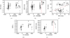 |
Fig. 5 HD 217987 summary. (a) RV time variations corrected from the secular acceleration drift. (b) BVS time variations, HARPS fiber change is shown with a vertical red line. (c) RV corrected from the secular acceleration drift vs BVS. The best linear fit is presentend in red dashed line. (d) log |

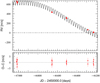 |
Fig. 6 Solution of HIP 36985 RV’s fit by a sum of two keplerians and its residuals |
4 Analysis
4.1 Stellar intrinsic variability
Figure 8 displays the mean RV uncertainty vs. B− V, v sin i and M*. We also display the RV rms vs. B−V, and age in Fig. 9. We observe that the mean RV uncertainty is correlated to the v sin i (Pearson = −0.65, pvalue ≪ 1%). This is consistent with what is observed on older, AF main sequence stars by Borgniet et al. (2017, 2019). We observe a strong jitter for most of the stars. The ratio between RV rms and the mean RV uncertainty is between 390 and 1 with a median at 16.
The median RV rms is 49 ms−1 (300 ms−1 on average). This jitter is mainly caused by pulsations for early type stars (from A to F5V), and by spots and faculae for late type stars (>F5V). Those two regimes can be distinguished, as stars with pulsations shows a vertical spread of BVS(RV) diagram, whereas stars with spots present a correlation between RV and BVS (Lagrange et al. 2009a). The main origin of RV jitter is reported in Table A.2 for each target.
78 stars out of 89 of our sample present variations in their Ca lines. The median log  of our sample is − 4.3 with a standard deviation of 0.2. 4 stars present signs of low activity (log
  < − 4.75), 59 are active (− 4.75 < log
  < −4.2) and 15 stars present signs of high activity (log
  > − 4.2). We present in Fig. 10 log
  vs. B−V. Some early F-type pulsating stars also present signs of actity when all late type stars present signs of activity.
HIP 36985B’s orbital parameters.
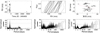 |
Fig. 7 BD+20 2465 summary. Top row: RV time variations, left: bisectors, middle: RV vs BVS (right). Bottom row: RV periodogram (left), BVS periodogram (middle), time window peridogram (right). The FAP at 1 and 10% are presented respectively in dashed lines and in dotted lines. |
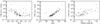 |
Fig. 8 Summary of the survey RV uncertainties. Mean RV uncertainty (accounting for the photon noise only) vs. B− V (left), vs. v sin i (middle) and vs. M⋆ (in M⊙, right). |
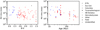 |
Fig. 9 Survey RV rms summary. Left: RV rms vs. B−V, right: RV rms and vs. age. Pulsating stars are plotted in blue, stars with RV dominated magnetic activity (spots) are plotted in red and stars with undetermined main source of RV are plotted in black. Stars with SB signature are not displayed (HD 106906, HD 131399, HD 177171). HD 197890 is not considered due to a too small set of data available. |
4.2 HARPS fiber change
In June 2015, the fiber of the HARPS instrument was changed in order to increase its stability (Lo Curto et al. 2015). Lo Curto et al. (2015) show that it leads to a change in the instrument profile which impacts the CCF computation and therefore the RV and BVS computation. They observed an offset in the RV between the datasets taken before and after this change of the order of 15 ms−1 for old F to K-type stars, based on 19 stars (Lo Curto et al. 2015). A more detailed analysis is currently underway for a large sample of close M-type main sequence stars (Mignon et al., in prep.). In this analysis, two reference spectra are computed, one before the change and one after. Our current set of spectra for each star is not big enough to build reference spectra as done in Mignon et al. (in prep.). The offset is different from one star to the other and its correlation with stellar parameters is not yet determined (spectral type, v sin i etc.). This offset has not been estimated on young stars before and the impact of high v sin i and strong jitter is not known. One should be careful before trying to correct this offset in order to not remove signal.
The difference between the mean of the RV before and after the fiber change can be measured, however, it won’t probe the offset alone, as long-term variations (star magnetic cycle, unseen companions, etc.) or a bad sampling of the jitter can also induce a difference in the mean of the RV.
We then decided to correct the offset only when it is significant enough. We compared the difference between the RV mean before and after the fiber change to the maximum of the rms before and after the fiber change to determine it. First, we selected the stars for which computing rms before and after the fiber change is relevant: we excluded the stars for which we have less than 10 spectra, less than 6 spectra before the fiber change, and less than 6 spectra after. We excluded the stars identified as SB (marked “B” in Table A.2) or presenting a long-term variation due to a companion (marked “T” in Table A.2). We also excluded the stars for which the RV amplitude is more than 900 ms−1 as the offset should be negligible compared to the jitter. We finally excluded HD 169178 that presents a trend due to a magnetic cycle. Finally, 29 stars were not excluded. We present the histogram of the ratio between the difference in mean of RV between before and after the fiber change and the maximum of the rms before and after the fiber change in Fig. 11. We chose to correct the RV offset for the stars that present a ratio larger than 1.3 a threshold that ensure a significant offset. Two stars correspond to this criterion. We present the characteristics of their offset in Table 2, and we present the correction of the offset for one of them in Fig. B.2. They have G to K-types and present an offset of the order of 50 ms−1. Such offsets are three times larger than those founds on old stars (Lo Curto et al. 2015).
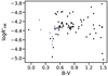 |
Fig. 10 Survey log |

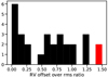 |
Fig. 11 Histogram of the ratio between the difference in the RV mean between before and after HARPS’ fiber change, andthe maximum of the rms before and after the fiber change. The stars that present a ratio greater than 1.3 are plotted in red. |
4.3 Exclusion of peculiar stars and RV correction for further analysis
In order to better estimate the number of potentially missed planets in our survey, we excluded some stars from our analyze and made some corrections on others before computing the detection limits. We excluded SB stars (HD 106906,HD 131399, HD 177171, HD 181321). Further, we excluded HD 116434 since its high value of v sin i (> 200 km s−1) prevents the measurements of BVS. We also excluded HD 197890 for which our data are too sparse to reliably quantify the detection limits (3 spectra). Thus leads to 83 stars, 23 A-F stars, 52 F-K stars, and 8 K-M stars.
For stars with RV dominated by spots (marked A in the Table A.2) we corrected their RV from the RV-BVS correlation using Melo et al. (2007) method (see Appendix B). We corrected HD 217987 RV from its proper motion and HD 186704 RV from its long-term trend with a linear regression. For β Pic, we considered the RV corrected from its pulsations as well as β Pic b and c contributions (Lagrange et al. 2019b).
For the stars for which we identified a non ambiguous offset in the RV, we corrected their RV from this offset (see Table 2).
Parameters of the stars that present a significant offset.
4.4 Detection limits
We compute mp sin i detection limits for periods between 1 and 1000 days in the GP domain (between 1 and 13MJup), and in the BD domain (between 13 and 80 MJup). We use the Local Power Analysis (LPA; Meunier et al. 2012; Borgniet et al. 2017) which determines, for all periods P, the minimum mp sin i for which a companion on a circular orbit with a period P would lead to a signal consistent with the data, by comparing the synthetic companion maximum power of its periodogram to the maximum power of the data periodogram within a small period range around the period P.
We then compute the completeness function C(mp sin i, P) which corresponds for a given couple (mp sin i, P) to the fraction of stars for which the companion is excluded by the detection limits (Borgniet et al. 2017). We present the 40–80% search completeness in Fig. 12.
4.5 Companion occurrence rates
We compute the upper limits of companions occurrence rates for our 83 stars in the GP (1–13 MJup) and BD (13–80 MJup) domains for AF (B−V ∈ [−0.05: 0.52]), FK (B−V ∈ [0.52: 1.33]), KM (B−V ≥ 1.33) type stars for different ranges of periods: 1–10, 10–100, 100–1000, and 1–1000 days. We use the method described in Borgniet et al. (2017) to compute the occurrence rates and to correct them from the estimated number of missed companions nmiss derived from the search completeness.
We present the upper limits of the occurrence rates for all stars in Fig. 13 and for AF, FK, M, and all stars in Table 3. The GP occurrence rate is below  (1σ) and the BD occurrence rate is below
  (1σ) for periods under 1000 days.
GP (mp sin i ∈ [1, 13] MJup) and BD (mp sin i ∈ [13, 80] MJup) occurrence rates around young nearby stars.
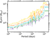 |
Fig. 12 Search completeness of our survey, corresponding to the lower mp sin i for which X% of the star of the survey have detection limits below this mp sin i at a given period P. From bottom to top 40–80%. |
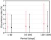 |
Fig. 13 Upper limits (1σ) on the occurrence rates for our survey for period ranges of 1–10, 10–100, and 100–1000 days in the GP domain (1−13 MJup, red) and BD domain (13−80 MJup, black). |
4.6 Comparaison to surveys on main sequence stars
No GP companion with periods lower than 1000 days was detected in the present survey. This non-detection is robust for HJ as 70% of the star of the survey have detection limits lower than 1 MJup for period lower than 10 days. The completeness of the survey is over 71% for AF and FK stars and nmiss < 0.4 for AF and FK stars in the 1–1000 days domain (cf. Table 3). However, we may have missed some planets with low masses and long period as only 40% of the stars of the survey have detection limits lower than 5 MJup between 100 and 1000 days.
We statistically tested if our GP non-detection implies GP occurrence rates around young stars significantly lower than around older main sequence (MS) stars, using the p-value formalism. The p-value is the probability to get the observed results given a null hypothesis, if it is lower than 10% then the null hypothesis can be rejected. We tested the following null hypothesis: GP occurrence rates are identical around young and main sequence stars in the same mass and period range.
We first applied this formalism in the 1–1000 days domain with a survey that have a completeness similar to ours. For AF MS stars the GP occurrence rate in this domain was estimated at  (Borgniet et al. 2019). We detected0 companion out of 23 stars, the corresponding p-value is
  . The null hypothesis can not be rejected.
Then, we applied this formalism in the HJ (P < 10 days) domain. For FK MS stars, the occurrence rate for HJ in this domain was estimated at:  by Cumming et al. (2008) and at 1.2 ± 0.38% by Wright et al. (2012). We detected 0 companion out of 52 stars, the corresponding p-value are respectively
  and
and  . The null hypothesis can not be rejected.
There is no evidence for a difference in occurrence rates of HJ between young and MS stars.
BD companions occurrence rates around MS stars is low:  for periods less than 1000 days (Borgniet et al. 2017), our non detection is not surprising. A bigger sample is needed to determine if BD occurrence rates around young and MS stars are different or not.
5 Conclusions
We observed 89 young A- to M-type stars over 3 yr or more with HARPS to search for GP and BD with periods less than 1000 days. This survey allowed to detect close binaries around HD 106906 and around HD 131399 (Lagrange et al. 2015, 2017). We constrained the period of HD 181321B and confirmed the RV trend in HD 186704’s RV. We also discovered a low-mass star companion to HIP 36985. No GP companion was detected in this survey. We obtain upper limits on the GP and BD occurrence rates, they are respectively  and
and  for periods of less than 1000 days. Our comparison of these occurrence rates to those derived for MS stars (Borgniet et al. 2019; Cumming et al. 2008; Wright et al. 2012) indicates that there is no evidence for a difference in occurrence rates of HJ between young and MS stars.
The forthcoming analysis of our SOPHIE survey around young stars and of our on-going HARPS survey on Sco-Cen stars will add 60 and 80 stars, respectively, in our analysis. This will allow for the derivation of more accurate occurrence rates and it will help in the search for the possible impact of system ages on occurrence rates.
Acknowledgements
We acknowledge support from the French CNRS and from the Agence Nationale de la Recherche (ANR grant GIPSE ANR-14-CE33-0018). This work has been supported by a grant from Labex OSUG@2020 (Investissements d’avenir – ANR10 LABX56). These results have made use of the SIMBAD database, operated at the CDS, Strasbourg, France. ESO SD acknowledges the support by INAF/Frontiera through the “Progetti Premiali” funding scheme of the Italian Ministry of Education, University, and Research.
Appendix A Sample
Stars characteristics for the 89 stars of our HARPS RV survey.
Results for the 89 stars of our HARPS RV survey.
Appendix B RV correction from the RV-BVS correlation
Solar to late-type stars present spots on their surfaces. These spots induce a quasi-periodic variations in the line profiles, which cause a signal in the RV and in the BVS. When the lines are resolved, there is at first order a correlation between the RV and the BVS (see Desort et al. 2007 for a detailed analysis).
To correct the RV signal induced by spots, we use Melo et al. (2007) method. It consists in correcting the RV from the linear regression of the RV vs. BVS dataset. The new RV at a given date t is:

where a and b are the slope and the intercept of the best linear fit of the RV vs. BVS dataset.
We present in Fig. B.1 an example of such correction for a star with v sin i = 31 km s−1. The mean RV rms of 300 ms−1 are reduced to 60 ms−1 after correction. This method was used in precedent works that use SAFIR (Lagrange et al. 2013; Borgniet et al. 2017, 2019).
We present a star for which a significant offset due to the HARPS fiber change is present in the corrected RV in Fig. B.2. The initial mean RV rms are 36 ms−1. After correction of the offset and of the RV-BVS correlation, the mean RV rms are 10 ms−1.
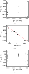 |
Fig. B.1 HD 102458 RV jitter correction. (a) RV time variations. (b) RV vs. BVS. The best linear fit is presentend in red dashed line. (c) RV corrected from the RV-BVS correlation. HARPS fiber change is shown with a vertical red line. |
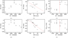 |
Fig. B.2 HD 218860 jitter and offset correction. (a) RV time variations. (b) RV vs. BVS. The best linear fit is presented in red dashed line. (c) RV corrected from the RV-BVS correlation. HARPS fiber change is shown with a vertical red line. (d) RVtime variations corrected from the offset due to the HARPS fiber change. (e) RV corrected from offset vs. BVS. The best linear fit is presented in red dashed line. (f) RV corrected from offset, corrected from their correlation to the BVS. HARPS fiber change is shown with a vertical red line. |
References
- Ammler-von Eiff, M., & Guenther, E. W. 2009, A&A, 508, 677 [NASA ADS] [CrossRef] [EDP Sciences] [Google Scholar]
- Aumann, H. H. 1985, PASP, 97, 885 [NASA ADS] [CrossRef] [Google Scholar]
- Backman, D. E., & Gillett, F. C. 1987, in Cool Stars, Stellar Systems and the Sun, Lecture Notes in Physics, eds. J. L. Linsky, & R. E. Stencel (Berlin: Springer Verlag), 291, 340 [NASA ADS] [CrossRef] [Google Scholar]
- Bailey, V., Meshkat, T., Reiter, M., et al. 2014, ApJ, 780, L4 [Google Scholar]
- Beichman, C. A., Bryden, G., Stapelfeldt, K. R., et al. 2006, ApJ, 652, 1674 [NASA ADS] [CrossRef] [Google Scholar]
- Beust, H., Lagrange-Henri, A. M., Vidal-Madjar, A., & Ferlet, R. 1989, A&A, 223, 304 [NASA ADS] [Google Scholar]
- Bonavita, M., Desidera, S., Thalmann, C., et al. 2016, A&A, 593, A38 [NASA ADS] [CrossRef] [EDP Sciences] [Google Scholar]
- Borgniet, S., Lagrange, A. M., Meunier, N., & Galland, F. 2017, A&A, 599, A57 [NASA ADS] [CrossRef] [EDP Sciences] [Google Scholar]
- Borgniet, S., Lagrange, A.-M., Meunier, N., et al. 2019, A&A, 621, A87 [NASA ADS] [CrossRef] [EDP Sciences] [Google Scholar]
- Bouchy, F., & Sophie Team. 2006, in Tenth Anniversary of 51 Peg-b: Status of and Prospects for Hot Jupiter Studies, eds. L. Arnold, F. Bouchy, & C. Moutou (Paris: Frontier Group), 319 [Google Scholar]
- Brandt, T. D., Kuzuhara, M., McElwain, M. W., et al. 2014, ApJ, 786, 1 [NASA ADS] [CrossRef] [Google Scholar]
- Carpenter, J. M., Bouwman, J., Mamajek, E. E., et al. 2009, ApJS, 181, 197 [NASA ADS] [CrossRef] [Google Scholar]
- Chauvin, G., Desidera, S., Lagrange, A.-M., et al. 2017a, in SF2A-2017: Proceedings of the Annual meeting of the French Society of Astronomy and Astrophysics, ed. C. Reylé, P. Di Matteo, F. Herpin, E. Lagadec, A. Lançon, Z. Meliani, & F. Royer, 331 [Google Scholar]
- Chauvin, G., Desidera, S., Lagrange, A.-M., et al. 2017b, A&A, 605, L9 [Google Scholar]
- Chen, C. H., Patten, B. M., Werner, M. W., et al. 2005, ApJ, 634, 1372 [NASA ADS] [CrossRef] [Google Scholar]
- Chen, C. H., Mittal, T., Kuchner, M., et al. 2014, ApJS, 211, 25 [NASA ADS] [CrossRef] [Google Scholar]
- Choquet, E., Perrin, M. D., Chen, C. H., et al. 2016, ApJ, 817, L2 [NASA ADS] [CrossRef] [Google Scholar]
- Churcher, L., Wyatt, M., & Smith, R. 2011, MNRAS, 410, 2 [NASA ADS] [CrossRef] [Google Scholar]
- Cumming, A., Butler, R. P., Marcy, G. W., et al. 2008, PASP, 120, 531 [CrossRef] [Google Scholar]
- de la Reza, R., & Pinzón, G. 2004, ApJ, 128, 1812 [NASA ADS] [CrossRef] [Google Scholar]
- Delorme, P., Lagrange, A. M., Chauvin, G., et al. 2012, A&A, 539, A72 [NASA ADS] [CrossRef] [EDP Sciences] [Google Scholar]
- Delorme, P., Schmidt, T., Bonnefoy, M., et al. 2017, A&A, 608, A79 [NASA ADS] [CrossRef] [EDP Sciences] [Google Scholar]
- Desidera, S., Covino, E., Messina, S., et al. 2015, A&A, 573, A126 [NASA ADS] [CrossRef] [EDP Sciences] [Google Scholar]
- Desort, M., Lagrange, A. M., Galland, F., Udry, S., & Mayor, M. 2007, A&A, 473, 983 [NASA ADS] [CrossRef] [EDP Sciences] [Google Scholar]
- Díez Alonso, E., Caballero, J. A., Montes, D., et al. 2019, A&A, 621, A126 [NASA ADS] [CrossRef] [EDP Sciences] [Google Scholar]
- Donaldson, J. K., Roberge, A., Chen, C. H., et al. 2012, ApJ, 753, 147 [NASA ADS] [CrossRef] [Google Scholar]
- Donati, J. F., Moutou, C., Malo, L., et al. 2016, Nature, 534, 662 [NASA ADS] [CrossRef] [Google Scholar]
- Esposito, M., Guenther, E., Hatzes, A. P., & Hartmann, M. 2006, in Tenth Anniversary of 51 Peg-b: Status of and Prospects for Hot Jupiter Studies, eds. L. Arnold, F. Bouchy, & C. Moutou (Paris: Frontier Group), 127 [Google Scholar]
- Figueira, P., Marmier, M., Bonfils, X., et al. 2010, A&A, 513, L8 [NASA ADS] [CrossRef] [EDP Sciences] [Google Scholar]
- Folsom, C. P., Bouvier, J., Petit, P., et al. 2018, MNRAS, 474, 4956 [NASA ADS] [CrossRef] [Google Scholar]
- Frankowski, A., & Jorissen, A. 2007, Balt. Astron., 16, 104 [NASA ADS] [Google Scholar]
- Fuhrmann, K., Chini, R., Kaderhandt, L., & Chen, Z. 2017, ApJ, 836, 139 [NASA ADS] [CrossRef] [Google Scholar]
- Gaia Collaboration (Brown, A. G. A., et al.) 2018, A&A, 616, A1 [NASA ADS] [CrossRef] [EDP Sciences] [Google Scholar]
- Galland, F., Lagrange, A. M., Udry, S., et al. 2005a, A&A, 443, 337 [NASA ADS] [CrossRef] [EDP Sciences] [Google Scholar]
- Galland, F., Lagrange, A. M., Udry, S., et al. 2005b, A&A, 444, L21 [NASA ADS] [CrossRef] [EDP Sciences] [Google Scholar]
- Gallet, F., & Bouvier, J. 2015, A&A, 577, A98 [NASA ADS] [CrossRef] [EDP Sciences] [Google Scholar]
- Golimowski, D. A., Krist, J. E., Stapelfeldt, K. R., et al. 2011, AJ, 142, 30 [NASA ADS] [CrossRef] [Google Scholar]
- Grandjean, A., Lagrange, A. M., Beust, H., et al. 2019, A&A, 627, L9 [NASA ADS] [CrossRef] [EDP Sciences] [Google Scholar]
- Guenther, E. W., & Esposito, E. 2007, ArXiv e-prints [arXiv:astro-ph/0701293] [Google Scholar]
- Hillenbrand, L. A., Carpenter, J. M., Kim, J. S., et al. 2008, ApJ, 677, 630 [Google Scholar]
- Hobbs, L. M., Vidal-Madjar, A., Ferlet, R., Albert, C. E., & Gry, C. 1985, ApJ, 293, L29 [NASA ADS] [CrossRef] [Google Scholar]
- Holland, W. S., Greaves, J. S., Zuckerman, B., et al. 1998, Nature, 392, 788 [Google Scholar]
- Huélamo, N., Figueira, P., Bonfils, X., et al. 2008, A&A, 489, L9 [NASA ADS] [CrossRef] [EDP Sciences] [Google Scholar]
- Kalas, P., Liu,M. C., & Matthews, B. C. 2004, Science, 303, 1990 [NASA ADS] [CrossRef] [PubMed] [Google Scholar]
- Kiefer, F., Lecavelier des Etangs, A., Boissier, J., et al. 2014, Nature, 514, 462 [NASA ADS] [CrossRef] [EDP Sciences] [Google Scholar]
- Kiraga, M. 2012, Acta Astron., 62, 67 [NASA ADS] [Google Scholar]
- Kley, W., & Nelson, R. P. 2012, ARA&A, 50, 211 [NASA ADS] [CrossRef] [Google Scholar]
- Koen, C., & Eyer, L. 2002, MNRAS, 331, 45 [NASA ADS] [CrossRef] [Google Scholar]
- Kovári, Z., Strassmeier, K., Granzer, T., et al. 2004, A&A, 417, 1047 [NASA ADS] [CrossRef] [EDP Sciences] [Google Scholar]
- Lagrange-Henri, A. M., Vidal-Madjar, A., & Ferlet, R. 1988, A&A, 190, 275 [NASA ADS] [Google Scholar]
- Lagrange, A. M., Desort, M., Galland, F., Udry, S., & Mayor, M. 2009a, A&A, 495, 335 [NASA ADS] [CrossRef] [EDP Sciences] [Google Scholar]
- Lagrange, A. M., Gratadour, D., Chauvin, G., et al. 2009b, A&A, 493, L21 [NASA ADS] [CrossRef] [EDP Sciences] [Google Scholar]
- Lagrange, A. M., De Bondt, K., Meunier, N., et al. 2012, A&A, 542, A18 [NASA ADS] [CrossRef] [EDP Sciences] [Google Scholar]
- Lagrange, A.-M., Meunier, N., Chauvin, G., et al. 2013, A&A, 559, A83 [NASA ADS] [CrossRef] [EDP Sciences] [Google Scholar]
- Lagrange, A.-M., Mathias, P., & Absil, O. 2015, A&A, submitted [Google Scholar]
- Lagrange, A.-M., Keppler, M., Beust, H., et al. 2017, A&A, 608, L9 [NASA ADS] [CrossRef] [EDP Sciences] [Google Scholar]
- Lagrange, A. M., Boccaletti, A., Langlois, M., et al. 2019a, A&A, 621, L8 [NASA ADS] [CrossRef] [EDP Sciences] [Google Scholar]
- Lagrange, A. M., Meunier, N., Rubini, P., et al. 2019b, Nat. Astron., 421 [Google Scholar]
- Lawler, S. M., Beichman, C. A., Bryden, G., et al. 2009, ApJ, 705, 89 [NASA ADS] [CrossRef] [Google Scholar]
- Lindgren, S., & Heiter, U. 2017, A&A, 604, A97 [NASA ADS] [CrossRef] [EDP Sciences] [Google Scholar]
- Lo Curto, G., Pepe, F., Avila, G., et al. 2015, The Messenger, 162, 9 [NASA ADS] [Google Scholar]
- Mamajek, E. E. 2012, ApJ, 754, L20 [NASA ADS] [CrossRef] [Google Scholar]
- Mamajek, E. E., Meyer, M. R., Hinz, P. M., et al. 2004, ApJ, 612, 496 [NASA ADS] [CrossRef] [Google Scholar]
- Mannings, V., & Barlow, M. J. 1998, ApJ, 497, 330 [NASA ADS] [CrossRef] [Google Scholar]
- Mayor, M., Pepe, F., Queloz, D., et al. 2003, The Messenger, 114, 2 [Google Scholar]
- McDonald, I., Zijlstra, A. A., & Boyer, M. L. 2012, MNRAS, 427, 343 [NASA ADS] [CrossRef] [Google Scholar]
- Melo, C., Santos, N. C., Gieren, W., et al. 2007, A&A, 467, 721 [NASA ADS] [CrossRef] [EDP Sciences] [Google Scholar]
- Meshkat, T., Bailey, V., Rameau, J., et al. 2013, ApJ, 775, L40 [NASA ADS] [CrossRef] [Google Scholar]
- Messina, S., Desidera, S., Turatto, M., Lanzafame, A. C., & Guinan, E. F. 2010, A&A, 520, A15 [NASA ADS] [CrossRef] [EDP Sciences] [Google Scholar]
- Messina, S., Millward, M., Buccino, A., et al. 2017, A&A, 600, A83 [NASA ADS] [CrossRef] [EDP Sciences] [Google Scholar]
- Meunier, N., Lagrange, A. M., & De Bondt, K. 2012, A&A, 545, A87 [NASA ADS] [CrossRef] [EDP Sciences] [Google Scholar]
- Meyer, M. R., Hillenbrand, L. A., Backman, D. E., et al. 2004, ApJS, 154, 422 [NASA ADS] [CrossRef] [Google Scholar]
- Meyer, M. R., Hillenbrand, L. A., Backman, D., et al. 2006, PASP, 118, 1690 [NASA ADS] [CrossRef] [Google Scholar]
- Meyer, M. R., Carpenter, J. M., Mamajek, E. E., et al. 2008, ApJ, 673, L181 [NASA ADS] [CrossRef] [Google Scholar]
- Milli, J., Hibon, P., Christiaens, V., et al. 2017, A&A, 597, L2 [NASA ADS] [CrossRef] [EDP Sciences] [Google Scholar]
- Montesinos, B., Eiroa, C., Mora, A., & Merín, B. 2009, A&A, 495, 901 [NASA ADS] [CrossRef] [EDP Sciences] [Google Scholar]
- Montet, B. T., Crepp, J. R., Johnson, J. A., Howard, A. W., & Marcy, G. W. 2014, ApJ, 781, 28 [NASA ADS] [CrossRef] [Google Scholar]
- Moór, A., Ábrahám, P., Kóspál, A., et al. 2013, ApJ, 775, L51 [NASA ADS] [CrossRef] [Google Scholar]
- Morales, F. Y., Bryden, G., Werner, M. W., & Stapelfeldt, K. R. 2016, ApJ, 831, 97 [NASA ADS] [CrossRef] [Google Scholar]
- Morin, J., Donati, J. F., Petit, P., et al. 2008, MNRAS, 390, 567 [NASA ADS] [CrossRef] [MathSciNet] [Google Scholar]
- Moro-Martín, A., Marshall, J. P., Kennedy, G., et al. 2015, ApJ, 801, 143 [NASA ADS] [CrossRef] [Google Scholar]
- Nidever, D. L., Marcy, G. W., Butler, R. P., Fischer, D. A., & Vogt, S. S. 2002, ApJS, 141, 503 [NASA ADS] [CrossRef] [Google Scholar]
- Nielsen, E. L., De Rosa, R. J., Rameau, J., et al. 2017, AJ, 154, 218 [Google Scholar]
- Nordström, B., Mayor, M., Andersen, J., et al. 2004, A&A, 418, 989 [NASA ADS] [CrossRef] [EDP Sciences] [Google Scholar]
- Olmedo, M., Chávez, M., Bertone, E., & De la Luz, V. 2013, PASP, 125, 1436 [NASA ADS] [CrossRef] [Google Scholar]
- Passegger, V. M., Reiners, A., Jeffers, S. V., et al. 2018, A&A, 615, A6 [NASA ADS] [CrossRef] [EDP Sciences] [Google Scholar]
- Patel, R. I., Metchev, S. A., & Heinze, A. 2014, ApJS, 212, 10 [NASA ADS] [CrossRef] [Google Scholar]
- Paulson, D. B., & Yelda, S. 2006, PASP, 118, 706 [NASA ADS] [CrossRef] [Google Scholar]
- Pecaut, M. J., Mamajek, E. E., & Bubar, E. J. 2012, ApJ, 746, 154 [NASA ADS] [CrossRef] [Google Scholar]
- Plavchan, P., Werner, M. W., Chen, C. H., et al. 2009, ApJ, 698, 1068 [NASA ADS] [CrossRef] [Google Scholar]
- Pollack, J. B., Hubickyj, O., Bodenheimer, P., et al. 1996, Icarus, 124, 62 [NASA ADS] [CrossRef] [Google Scholar]
- Poveda, A., Allen, C., Costero, R., Echevarría, J., & Hernández-Alcántara, A. 2009, ApJ, 706, 343 [NASA ADS] [CrossRef] [Google Scholar]
- Rameau, J., Chauvin, G., Lagrange, A.-M., et al. 2013a, ApJ, 772, L15 [NASA ADS] [CrossRef] [Google Scholar]
- Rameau, J., Chauvin, G., Lagrange, A. M., et al. 2013b, A&A, 553, A60 [NASA ADS] [CrossRef] [EDP Sciences] [Google Scholar]
- Rebull, L. M., Stapelfeldt, K. R., Werner, M. W., et al. 2008, ApJ, 681, 1484 [NASA ADS] [CrossRef] [Google Scholar]
- Rebull, L. M., Stauffer, J. R., Bouvier, J., et al. 2016, AJ, 152, 114 [NASA ADS] [CrossRef] [Google Scholar]
- Rhee, J. H., Song, I., Zuckerman, B., & McElwain, M. 2007, ApJ, 660, 1556 [NASA ADS] [CrossRef] [MathSciNet] [Google Scholar]
- Rodet, L., Beust, H., Bonnefoy, M., et al. 2017, A&A, 602, A12 [NASA ADS] [CrossRef] [EDP Sciences] [Google Scholar]
- Schneider, G., Silverstone, M. D., Hines, D. C., et al. 2006, ApJ, 650, 414 [NASA ADS] [CrossRef] [Google Scholar]
- Ségransan, D., Mayor, M., Udry, S., et al. 2011, A&A, 535, A54 [NASA ADS] [CrossRef] [EDP Sciences] [Google Scholar]
- Sierchio, J. M., Rieke, G. H., Su, K. Y. L., & Gáspár, A. 2014, ApJ, 785, 33 [NASA ADS] [CrossRef] [Google Scholar]
- Simon, M., & Schaefer, G. H. 2011, ApJ, 743, 158 [NASA ADS] [CrossRef] [Google Scholar]
- Smith, B. A., & Terrile, R. J. 1984, Science, 226, 1421 [NASA ADS] [CrossRef] [PubMed] [Google Scholar]
- Soto, M. G., Jenkins, J. S., & Jones, M. I. 2015, MNRAS, 451, 3131 [NASA ADS] [CrossRef] [Google Scholar]
- Soummer, R., Perrin, M. D., Pueyo, L., et al. 2014, ApJ, 786, L23 [NASA ADS] [CrossRef] [Google Scholar]
- Stauffer, J., Rebull, L., Bouvier, J., et al. 2016, AJ, 152, 115 [NASA ADS] [CrossRef] [Google Scholar]
- Strassmeier, K. G., Pichler, T., Weber, M., & Granzer, T. 2003, A&A, 411, 595 [NASA ADS] [CrossRef] [EDP Sciences] [Google Scholar]
- Teyssandier, J., Lai, D., & Vick, M. 2019, MNRAS, 486, 2265 [NASA ADS] [CrossRef] [Google Scholar]
- Tokovinin, A. 2014, AJ, 147, 87 [NASA ADS] [CrossRef] [Google Scholar]
- Tremko, J., Bakos, G. A., Žižňovský, J., & Pribulla, T. 2010, Contrib. Astron. Observ. Skalnate Pleso, 40, 83 [NASA ADS] [Google Scholar]
- van Leeuwen, F. 2007, A&A, 474, 653 [NASA ADS] [CrossRef] [EDP Sciences] [Google Scholar]
- Vigan, A., Bonavita, M., Biller, B., et al. 2017, A&A, 603, A3 [NASA ADS] [CrossRef] [EDP Sciences] [Google Scholar]
- Wagner, K., Apai, D., Kasper, M., et al. 2016, Science, 353, 673 [NASA ADS] [CrossRef] [Google Scholar]
- Weise, P., Launhardt, R., Setiawan, J., & Henning, T. 2010, A&A, 517, A88 [NASA ADS] [CrossRef] [EDP Sciences] [Google Scholar]
- Wright, N. J., Drake, J. J., Mamajek, E. E., & Henry, G. W. 2011, ApJ, 743, 48 [NASA ADS] [CrossRef] [Google Scholar]
- Wright, J. T., Marcy, G. W., Howard, A. W., et al. 2012, ApJ, 753, 160 [NASA ADS] [CrossRef] [Google Scholar]
- Yu, L., Donati, J.-F., Hébrard, E. M., et al. 2017, MNRAS, 467, 1342 [NASA ADS] [Google Scholar]
- Zuckerman, B., & Song, I. 2004, ApJ, 603, 738 [NASA ADS] [CrossRef] [Google Scholar]
- Zuckerman, B., Rhee, J. H., Song, I., & Bessell, M. S. 2011, ApJ, 732, 61 [NASA ADS] [CrossRef] [Google Scholar]
- Zuckerman, B., Vican, L., Song, I., & Schneider, A. 2013, ApJ, 778, 5 [NASA ADS] [CrossRef] [Google Scholar]
All Tables
GP (mp sin i ∈ [1, 13] MJup) and BD (mp sin i ∈ [13, 80] MJup) occurrence rates around young nearby stars.
All Figures
|
Fig. 1 Main physical properties of our sample. (a) Absolute V -magnitude vs. B− V. Each black dot corresponds to one target. The Sun is displayed (red star) for comparison. (b) v sin i vs B− V distribution. (c) Mass histogram (in M⊙). (d) Age histogram. |
| In the text | |
|
Fig. 2 Observation summary. (a) Histogram of the number of spectra per target, excluding HD 216956 (Fomalhaut, 834 spectra) and HD 039060 (β Pic, 5108 spectra). (b) Histogram of the number of nights per target. (c) Histogram of the time baselines. |
| In the text | |
|
Fig. 3 HD 186704 RV long term trend. Left: RV time variations, right: RV corrected from the RV-BVS correlation time variations. |
| In the text | |
|
Fig. 4 Solutions of HD 181321 RV fit by the sum of two Keplerian (top) and their residuals (bottom). Left: 1600 days solution. Right: 3200 days solution. |
| In the text | |
|
Fig. 5 HD 217987 summary. (a) RV time variations corrected from the secular acceleration drift. (b) BVS time variations, HARPS fiber change is shown with a vertical red line. (c) RV corrected from the secular acceleration drift vs BVS. The best linear fit is presentend in red dashed line. (d) log |
| In the text | |
|
Fig. 6 Solution of HIP 36985 RV’s fit by a sum of two keplerians and its residuals |
| In the text | |
|
Fig. 7 BD+20 2465 summary. Top row: RV time variations, left: bisectors, middle: RV vs BVS (right). Bottom row: RV periodogram (left), BVS periodogram (middle), time window peridogram (right). The FAP at 1 and 10% are presented respectively in dashed lines and in dotted lines. |
| In the text | |
|
Fig. 8 Summary of the survey RV uncertainties. Mean RV uncertainty (accounting for the photon noise only) vs. B− V (left), vs. v sin i (middle) and vs. M⋆ (in M⊙, right). |
| In the text | |
|
Fig. 9 Survey RV rms summary. Left: RV rms vs. B−V, right: RV rms and vs. age. Pulsating stars are plotted in blue, stars with RV dominated magnetic activity (spots) are plotted in red and stars with undetermined main source of RV are plotted in black. Stars with SB signature are not displayed (HD 106906, HD 131399, HD 177171). HD 197890 is not considered due to a too small set of data available. |
| In the text | |
|
Fig. 10 Survey log |
| In the text | |
|
Fig. 11 Histogram of the ratio between the difference in the RV mean between before and after HARPS’ fiber change, andthe maximum of the rms before and after the fiber change. The stars that present a ratio greater than 1.3 are plotted in red. |
| In the text | |
|
Fig. 12 Search completeness of our survey, corresponding to the lower mp sin i for which X% of the star of the survey have detection limits below this mp sin i at a given period P. From bottom to top 40–80%. |
| In the text | |
|
Fig. 13 Upper limits (1σ) on the occurrence rates for our survey for period ranges of 1–10, 10–100, and 100–1000 days in the GP domain (1−13 MJup, red) and BD domain (13−80 MJup, black). |
| In the text | |
|
Fig. B.1 HD 102458 RV jitter correction. (a) RV time variations. (b) RV vs. BVS. The best linear fit is presentend in red dashed line. (c) RV corrected from the RV-BVS correlation. HARPS fiber change is shown with a vertical red line. |
| In the text | |
|
Fig. B.2 HD 218860 jitter and offset correction. (a) RV time variations. (b) RV vs. BVS. The best linear fit is presented in red dashed line. (c) RV corrected from the RV-BVS correlation. HARPS fiber change is shown with a vertical red line. (d) RVtime variations corrected from the offset due to the HARPS fiber change. (e) RV corrected from offset vs. BVS. The best linear fit is presented in red dashed line. (f) RV corrected from offset, corrected from their correlation to the BVS. HARPS fiber change is shown with a vertical red line. |
| In the text | |
Current usage metrics show cumulative count of Article Views (full-text article views including HTML views, PDF and ePub downloads, according to the available data) and Abstracts Views on Vision4Press platform.
Data correspond to usage on the plateform after 2015. The current usage metrics is available 48-96 hours after online publication and is updated daily on week days.
Initial download of the metrics may take a while.