© ESO 2020

1. Introduction

There is growing evidence that a warm optically thick corona exists in accreting black holes when an accretion disk is present. It is observed in different types of accreting black holes across various masses: active galactic nuclei (AGN; Pounds et al. 1987; Magdziarz et al. 1998; Mehdipour et al. 2011; Done et al. 2012; Petrucci et al. 2013, 2018; Keek & Ballantyne 2016) including quasars (Madau 1988; Laor et al. 1994, 1997; Gierliński & Done 2004; Piconcelli et al. 2005), ultraluminous X-ray sources (ULXs; Goad et al. 2006; Stobbart et al. 2006; Gladstone et al. 2009), and galactic black hole binaries (GBHBs; Gierliński et al. 1999; Zhang et al. 2000; Di Salvo et al. 2001). A warm corona is visible as a soft component (below 2 keV) in the X-ray spectra of these objects. It is generally characterized by an excess with respect to the extrapolation of a hard X-ray power law. This power law typically originates from a region called hot corona.

The observed spectral shape of the soft X-ray excess provides us some insight into the radiative cooling mechanism that operates in the warm corona. Assuming that the thermal Comptonization is the dominant cooling process, we can model the observed spectra with so-called slab model, where soft photons from the disk enter the warm corona that is located above the disk and undergo Compton scattering with amplification factor y. During the fitting procedure, the temperature and optical depth of a warm corona can be determined. Observations of many sources indicate that a corona like this has an optical depth ranging from 4 up to 40 in different objects (Zhang et al. 2000; Jin et al. 2012; Petrucci et al. 2013, 2018, and references therein).

Furthermore, observations constrain the amount of energy that is dissipated in corona, f, in comparison to the total energy released in the whole disk or corona system. Observations of GBHBs and AGNs show that f ≈ 1 is required to explained the observed spectral index α = 0.9 in some sources (Haardt & Maraschi 1991; Życki et al. 2001; Petrucci et al. 2013). Petrucci et al. (2018) set a lower limit of f = 0.8. This behavior is not universal because it depends on the object and its spectral state, but it shows that in some circumstances, much energy is released outside of an accretion disk.

The more fundamental question is how this warm optically thick slab of gas can be created above an accretion disk that has a lower temperature. The additional process that heats the warm corona and maintains it in steady state with disk is also unclear.

Many attempts have been made to determine the universal mechanism of energy dissipation in the warm corona, but the problem is still not fully solved. A strong corona, which is responsible for most of the thermal energy that is released increases the disk stability (Svensson & Zdziarski 1994; Kusunose & Mineshige 1994; Begelman & Pringle 2007). However, detailed computations of radiative transfer in illuminated accretion disk atmospheres show that the outer warm or hot skin cannot be optically thick and stable at the same time (Ballantyne et al. 2001; Nayakshin & Kallman 2001; Różańska et al. 2002, 2015; Madej & Różańska 2004). When the irradiation increases, the ionized skin becomes unstable and the gas most probably flows out in the form of wind (Proga & Waters 2015). Computations show that the warm or hot skin with an optical depth higher than 3 cannot be thermally stable (in pressure equillibrium) with a cold accretion disk when the skin is heated only radiatively (Krolik & Kriss 1995; Nayakshin et al. 2000; Różańska et al. 2002, 2015, and references therein).

Additional heating of the warm corona layer by an accretion process has also been considered. However, Shakura & Sunyaev (1973) introduced the geometrically thin-disk model in their seminal paper, where the kinetic energy of accreting gas is locally converted into thermal energy. According to this, within the standard disk model all energy is dissipated deep inside the disk at the equatorial plane. Vertical profiles of energy dissipation clearly show the exponential decrease toward the disk surface.

The development of numerical simulations has shown the role of the magnetic field in the structure of the accretion disk (Hawley & Balbus 1991; Balbus & Hawley 1991; Tout & Pringle 1992; Hawley 2001; Stone et al. 2008). Many magnetohydrodynamic (MHD) simulations are available, but none of them specifies the optical depth of the warm corona because most of them do not take radiative cooling into account (e.g., Bai & Stone 2013; Penna et al. 2013). The simulations that contain simplified radiative cooling (e.g., Turner 2004; Hirose et al. 2009; Ohsuga & Mineshige 2011; Noble et al. 2011) only discuss a hot corona without constrains on its observational properties (i.e., Jiang et al. 2014; Sądowski et al. 2017). Highly advanced radiative transfer calculations are usually made a posteriori after general relativistic MHD simulations are completed (Schnittman et al. 2016).

Różańska et al. (2015, hereafter RMB15) have developed an analytic model for an optically thick uniformly heated Compton-cooled corona in hydrostatic equilibrium. The heating mechanism was not specified in the model, but it allowed the authors to integrate vertically both disk and warm corona, coupled by mechanical heating and radiative cooling. This allowed them to determine the relations between the optical depth of the warm layer and the disk-corona energy budget. Furthermore, the authors have shown that when some part of the gas pressure is replaced by magnetic pressure, the optical depth of the stable corona increases.

We here assume a geometrically thin and optically thick accretion disk around a black hole (see Fig. 1). We also assume that the accretion disk is magnetized and the magneto-rotational instability (MRI) is the primary source of viscosity and energy dissipation. Based on these assumptions, we develop the model of a slab-like warm corona that covers the accretion disk and adopt realistic heating of the gas by magnetic field reconnection, which in contrast to the standard disk increases toward the disk surface (Hirose et al. 2006). We directly use the analytic formula derived by Begelman et al. (2015, hereafter BAR15), where the vertical profile of the magnetic heating of the accretion flow is determined. In addition to this major assumption, the vertical structure of the disk together with the radiative transfer equation in a gray atmosphere are fully solved with the relaxation method proposed by Henyey et al. (1964). We have developed a new numerical scheme that allows solving nonlinear differential equations in a relatively short time, which keeps the integration error low. Furthermore, with our new method we are able to pass through the thermally unstable regions that may arise when nonuniform heating and cooling mechanisms take place.

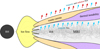Fig. 1. Schematic illustration of a slice through the disk plane (only one side is shown due to symmetry). The black hole is shown as the circle on the left. The gray area represents the optically thick and geometrically thin disk where most of the accreting mass is located. The warm corona that covers the disk, in which the magnetic energy is released as radiation, is marked in orange. Magnetic and radiative energy flux are represented by blue and red arrows, respectively. The part of the corona that might collapse as a result of thermal instability is shown in magenta. The inner optically thin and geometrically thick hot flow that we did not consider is drawn in yellow for completion.

As a result, we show for which range of parameters a warm corona can exist in case of a GBHB. We determine the optical depth of the warm layer, which is the main observable when X-ray data are analyzed. Detailed calculations of the vertical structure allow us to estimate the amount of energy that is dissipated in the corona in comparison to the total energy that is released by accretion at a given radius. We show the radial structure of an optically thick corona and give tight constraints for conditions for which this warm layer can exist. All results are compared with observations.

A warm corona is not the only possible model with which the soft X-ray excess can be explained. Other models assume relativistically smeared absorption (Gierliński & Done 2004) or reflection from an accretion disk that is illuminated by a hard X-ray continuum (García et al. 2019) or bulk Comptonization in a central Compton cloud (Shaposhnikov & Titarchuk 2006; Seifina et al. 2016). All of these models provide good fits to X-ray observations by incorporating an additional Comptonized component, but they do not explain the physical mechanism that feeds energy into the warm gas to compensate for the huge rate of the Compton cooling. Models that do provide the heating mechanism for a central compact corona exist and can successfully explain some observations without the need of involving the magnetic field (Seifina et al. 2018). However, we note that the role of the magnetic field in the accretion and jet formation process has been shown numerous times in the papers cited in this section, and we do not consider it a strong assumption. We show that an accretion disk with an operating magnetic dynamo is able to produce enough energy to heat the extended surface layer, whose physical parameters are consistent with those determined from spectral fitting of observations. Our results give a possible physical explanation for the phenomenon that was in most cases only considered from an observational perspective without analyzing the global energy budget. In order to verify whether our model can correctly reproduce the spectral features seen in X-ray sources, spectral modeling involving the redistribution function of Compton scattering must be performed. This is beyond the scope of this paper, however.

The structure of the paper is as follows: Sect. 2 presents the formalism of a magnetically heated corona and the disk-corona radiative transfer equation. It ends with a full description of the differential equations and the relaxation method we used to solve them. Section 3 presents the results of our numerical computations. We display the vertical structure of the disk-corona system, but we also show the radial limitation within which an optically thick corona can exist. Discussion and conclusions are given in Sect. 4.

2. Model setup

2.1. Magnetically heated corona

Begelman & Pringle (2007) and later BAR15 have proposed a vertical model of magnetically supported disks (MSDs) that are driven by the MRI dynamo. The MRI dynamo operating near the equatorial plane in the presence of an external poloidal magnetic field generates the toroidal magnetic flux, which converts the mechanical energy of the accretion into the electromagnetic energy that is stored as tangled magnetic field lines. The total rate of this energy deposition per unit height is α_BΩP_tot, where α_B is the toroidal magnetic field production parameter, Ω is the Keplerian angular velocity, and P_tot is the total pressure, which is the sum of gas, radiation, and magnetic pressure. Although the toroidal field production parameter α_B does resemble the effective viscosity parameter α = t_rϕ/P (known from the classical thin-disk model) in the sense that it scales the energy release within the disk, its physical meaning is different, even though the expected values of both parameters are similar (Salvesen et al. 2016, hereafter SSAB16, Table 3).

The magnetic flux ropes that form near the midplane rise buoyantly toward the surface, and in the model by BAR15, the velocity is very coarsely approximated by

$$\begin{array}{c}\hfill v_{\mathrm{B}}(z)=\eta \mathrm{\Omega }z,\end{array}$$(1)

where 0 <  η <  1 is a dimensionless parameter. A similar process of a buoyant emergence of magnetic fields toward the surface is observed on the Sun, but the dynamical properties and the origin of the magnetic field are vastly different.

During the upward motion of the ropes, the magnetic field decays by various processes, releasing its accumulated energy into heating the gas. When we assume a purely toroidal flux that rises vertically with speed v_B(z), the energy dissipation rate due to the induced current, ℋ_mag, can be derived from the elemental electrodynamics and yields

$$\begin{array}{c}\hfill {\mathcal{H}}_{\mathrm{mag}}=-v_{\mathrm{B}}\mathrm{d}{P}_{\mathrm{mag}}/\mathrm{d}z.\end{array}$$(2)

This expression is consistent with intuitive reasoning: the energy loss is proportional to the magnetic energy density gradient times velocity.

Another process that may heat the gas is magnetic reconnection due to cyclic reversals of the toroidal field polarity that is observed in simulations of the MRI dynamo. The energy output of this process is proportional to the magnetic pressure P_mag and can be estimated as

$$\begin{array}{c}\hfill {\mathcal{H}}_{\mathrm{rec}}=2\xi \mathrm{\Omega }{P}_{\mathrm{mag}},\end{array}$$(3)

where ξ is a proportionality constant (Appendix A in BAR15). The rate of thermal energy release peaks in the proximity of the disk photosphere (τ = 1), but its exact distribution may change depending on the model parameters. Alongside ξ, we also define, after BAR15, the reconnection efficiency parameter ν, which describes the ratio of reconnection process to the total magnetic viscosity: ν = 2ξ/α_B, and it is very convenient to present our results (see Sect. 3.5).

One consequence of this picture is that the field outflow eventually reaches the point where heating becomes inefficient and some portion of the accretion energy may be carried away by the Poynting flux and is never released to heat the gas. This is contrary to nonmagnetic classical (neglecting advection) α-viscosity models where all accretion power is released as radiation. The magnetic outflow may be associated with the matter outflow, but this association is not trivial: because the outflow speed v_B is lower than the freefall speed v_ff = Ωz, most of the matter will probably slide down the magnetic flux tubes, and only a small amount is carried away by the outflow. In contrast, during the mass ejections in the solar corona, the eruption timescale is much shorter than the dynamical timescale, which results in much more efficient mass transport.

Numerical modeling shows that the process described above can be very complex, but this analytic approximation enables us to build and study the atmospheres of MSDs, which is the purpose of this paper.

Following BAR15, the accretion energy is injected into the Poynting flux and consumed for gas heating, in varying proportion. When we express the Poynting flux as F_mag = 2P_magv_B, the magnetic energy conservation equation can be written as

$$\begin{array}{cc}\hfill {\alpha }_{\mathrm{B}}\mathrm{\Omega }{P}_{\mathrm{tot}}& =\frac{\mathrm{d}{F}_{\mathrm{mag}}}{\mathrm{d}z}+{\mathcal{H}}_{\mathrm{rec}}+{\mathcal{H}}_{\mathrm{mag}}\hfill \\ \hfill & =\frac{\mathrm{d}}{\mathrm{d}z}\left(2P_{\mathrm{mag}}{v}_{\mathrm{B}}\right)+(2\xi \mathrm{\Omega }{P}_{\mathrm{mag}}-v_{\mathrm{B}}\frac{\mathrm{d}{P}_{\mathrm{mag}}}{\mathrm{d}z})·\hfill \end{array}$$(4)

We substitute velocity and different energy rates by Eqs. (1)–(3) to obtain the final expression for the magnetic pressure gradient,

$$\begin{array}{c}\hfill \eta \mathrm{\Omega }z\frac{\mathrm{d}{P}_{\mathrm{mag}}}{\mathrm{d}z}={\alpha }_{\mathrm{B}}\mathrm{\Omega }{P}_{\mathrm{tot}}-(2\eta +{\alpha }_{\mathrm{B}}\nu )\mathrm{\Omega }{P}_{\mathrm{mag}}.\end{array}$$(5)

Finally, we can use this equation to obtain the expression for the heating rate ℋ [erg cm⁻³ s⁻¹] without using gradients,

$$\begin{array}{c}\hfill \mathcal{H}={\mathcal{H}}_{\mathrm{rec}}+{\mathcal{H}}_{\mathrm{mag}}=2(\eta +{\alpha }_{\mathrm{B}}\nu )\mathrm{\Omega }{P}_{\mathrm{mag}}-{\alpha }_{\mathrm{B}}\mathrm{\Omega }{P}_{\mathrm{tot}}.\end{array}$$(6)

This heating rate describes the amount of released magnetic energy that heats the gas and can then be converted into radiation. In this paper we neglect advection and assume that the system is fully cooled by radiation, as specified in the next section.

2.2. Radiative transfer in the disk-corona system

We consider a gray plane-parallel optically thick atmosphere, which is additionally heated by dissipation of the magnetic field. We include free-free process and Compton scattering in our model and neglect synchrotron radiation, which is not important in this regime of magnetic pressure (see Sect. 3.1 for exact numbers). To determine the temperature structure, we consider three equations: a radiative equilibrium equation, a transfer equation, and an Eddington approximation.

The radiative equilibrium equation for a small-matter volume heated by various dissipation processes at rate ℋ and by the local radiation field of mean intensity J_ν and cooled by the radiation emissivity j_ν reads

$$\begin{array}{c}\hfill 4\pi {\displaystyle {\int }_{\nu }{\kappa }_{\nu }\rho J_{\nu }\mathrm{d}\nu +\mathcal{H}=4\pi j_{\mathrm{bol}},}\end{array}$$(7)

where j_bol ≡ ∫_νj_νdν, and ρ is gas density in g cm⁻³. Here, we assumed that the entire dissipated thermal energy is locally converted into radiation (neglecting advection).

In an optically thick regime, when true absorption processes dominate scattering, the radiation field is fully thermalized and strictly local, therefore for matter at temperature T, we have J_ν = B_ν(T), where B_ν(T) is the Planck function for temperature T. However, because a corona is a strongly scattering medium, this is not the case (particularly near the surface), and the actual radiation field intensity may deviate from a Planck distribution toward a Wien distribution. The further deviation from the Planck law is caused by non-coherent inverse Compton scattering. We still assume that the spectrum of mean radiation intensity J_ν within the disk can be approximately described by the Planck function with temperature T_rad, that is, J_ν ≈ B_ν(T_rad). With these assumptions, we can define our frequency-averaged quantities

$$B={\displaystyle {\int }_0^{\infty }{B}_{\nu }}\text{d}\nu ={\displaystyle {\int }_0^{\infty }{B}_{\nu }}(T)\text{d}\nu =\sigma T^4/\pi ,$$(8)

$$J={\displaystyle {\int }_0^{\infty }{J}_{\nu }}\text{d}\nu ={\displaystyle {\int }_0^{\infty }{B}_{\nu }}(T_{\text{rad}})\text{d}\nu =\sigma T_{\text{rad}}^4/\pi .$$(9)

Even when we assume that the radiation field has a Planck distribution, we do not equal gas and radiation temperatures because the corona is strongly dominated by scattering.

For the gray atmosphere we considered in this paper, we used both Rosseland and Planck averages, the latter denoted with a “P” superscript. The following values for electron scattering and free-free opacities were assumed:

$${\kappa }_{\text{es}}=0.34{\text{g}}^{-1}{\text{cm}}^2,$$(10)

$${\kappa }_{\text{ff}}^{\text{P}}=37\cdot {\kappa }_{\text{ff}}={\kappa }_{\text{ff},\text{0}}^{\text{P}}\cdot \rho T^{-7/2}{\text{g}}^{-1}{\text{cm}}^2,$$(11)

where ${\kappa }_{\mathrm{ff},0}^{\mathrm{P}}=37\times 6.21\times {10}^{22}$ is a constant from Kramers opacity approximation in cgs units. Through this paper, we denote the total Rosseland mean opacity as κ = κ_es + κ_ff, while ${\kappa }^{\mathrm{P}}={\kappa }_{\mathrm{es}}+{\kappa }_{\mathrm{ff}}^{\mathrm{P}}$ is the total Planck opacity.

Using the gray approximation, we can rewrite the radiative equilibrium Eq. (7) as

$$\begin{array}{c}\hfill \mathcal{H}=4\pi (j_{\mathrm{bol}}-{\kappa }^{\mathrm{P}}\rho J)\equiv {\mathrm{\Lambda }}_{\mathrm{rad}}(\rho ,T,T_{\mathrm{rad}}).\end{array}$$(12)

We refer to the function Λ_rad(ρ, T, T_rad) as the net radiative cooling rate.

To estimate the effect of inverse Compton scattering, we used the standard formula given by Rybicki & Lightman (2008), where by J_C we mean all incident photons that were scattered with thermalized electrons of the gas temperature T:

$$\begin{array}{c}\hfill J_{\mathrm{C}}^{\prime }-J_{\mathrm{C}}=J_{\mathrm{C}}\frac{4kT⟨\epsilon ⟩-⟨{\epsilon }^2⟩}{⟨\epsilon ⟩m_e{c}^2}·\end{array}$$(13)

In this formula $J_{\text{C}}^{\prime }-J_{\text{C}}$ is the energy passed to the radiation from electrons by the inverse Compton scattering. The mean photon energy ⟨ε⟩ and mean squared energy ⟨ε²⟩ depend on the photon energy distribution, and their ratio has the following values:

$$\begin{array}{c}\hfill ⟨{\epsilon }^2⟩=\{\begin{array}{cc}3.83k{T}_{\mathrm{rad}}·⟨\epsilon ⟩\hfill & \text{for a Planck spectrum}\hfill \\ 4k{T}_{\mathrm{rad}}·⟨\epsilon ⟩\hfill & \text{for a Wien spectrum}.\hfill \end{array}\end{array}$$(14)

Although we assumed that the radiation has a Planck spectrum everywhere in the atmosphere, for a strongly scattering medium with a Compton-cooled corona, the radiation spectrum is shifted toward slightly higher energies, and we find the approximation ⟨ε²⟩ = 4kT_rad ⋅ ⟨ε⟩ satisfactory for our model. When the temperatures are low, density is high, and free-free absorption dominates, this term is negligible and does not change the result. Therefore we replace J_C = κ_esJ to obtain the Compton term for the emission function,

$$\begin{array}{c}\hfill j_{\mathrm{IC}}={\kappa }_{\mathrm{es}}J\frac{4k(T-T_{\mathrm{rad}})}{m_e{c}^2}·\end{array}$$(15)

Finally, by taking into account all relevant opacities, we obtain the emission function j_bol of the following form:

$$\begin{array}{c}\hfill j_{\mathrm{bol}}={\kappa }_{\mathrm{ff}}^{\mathrm{P}}B+{\kappa }_{\mathrm{es}}J+j_{\mathrm{IC}}={\kappa }_{\mathrm{ff}}^{\mathrm{P}}B+{\kappa }_{\mathrm{es}}J[1+\frac{4k(T-T_{\mathrm{rad}})}{m_e{c}^2}]·\end{array}$$(16)

We can now substitute the expressions for B, J, and j_bol into the cooling function Λ_rad to obtain its final form,

$$\begin{array}{cc}& {\mathrm{\Lambda }}_{\mathrm{rad}}(\rho ,T,T_{\mathrm{rad}})\equiv 4\sigma \rho [{\kappa }_{\mathrm{ff}}^{\mathrm{P}}(T^4-T_{\mathrm{rad}}^4)+{\kappa }_{\mathrm{es}}{T}_{\mathrm{rad}}^4\frac{4k(T-T_{\mathrm{rad}})}{m_e{c}^2}]\hfill \\ \hfill & =4\sigma \rho (T-T_{\mathrm{rad}})[{\kappa }_{\mathrm{ff}}^{\mathrm{P}}(T+T_{\mathrm{rad}})(T^2+T_{\mathrm{rad}}^2)+{\kappa }_{\mathrm{es}}\frac{4k{T}_{\mathrm{rad}}^4}{m_e{c}^2}]·\hfill \end{array}$$(17)

The net cooling rate can be split into two terms: Λ_rad = Λ_B + Λ_C, describing the contributions of bremsstrahlung and Compton scattering,

$${\mathrm{\Lambda }}_{\text{B}}=4\sigma \rho {\kappa }_{\text{ff}}^{\text{P}}\left(T^4-T_{\text{rad}}^4\right),$$(18)

$${\mathrm{\Lambda }}_{\text{C}}=4\sigma \rho {\kappa }_{\text{es}}{T}_{\text{rad}}^4\frac{4k\left(T-T_{\text{rad}}\right)}{m_e{c}^2}\cdot$$(19)

We solve here the frequency-integrated radiative transfer equation (Eq. (4) in RMB15), where the zeroth moment of this equation reads

$$\begin{array}{c}\hfill \frac{\mathrm{d}H}{\mathrm{d}z}=j_{\mathrm{bol}}-{\kappa }^P\rho J.\end{array}$$(20)

When we average this over the frequencies and replace the Eddington flux with a physical flux 4πH_Edd = F_rad, we obtain the expected result that the energy gained by the radiative flux is equal to the rate of radiative gas cooling,

$$\begin{array}{c}\hfill \frac{\mathrm{d}{F}_{\mathrm{rad}}}{\mathrm{d}z}={\mathrm{\Lambda }}_{\mathrm{rad}}(\rho ,T,T_{\mathrm{rad}}).\end{array}$$(21)

Because we are interested in the optically thick regime, we assume the Eddington approximation, that is, J = 3 K, where K is the second moment of specific intensity. We therefore solve the first moment of the radiative transfer equation as

$$\begin{array}{c}\hfill \frac{1}{3}\frac{\mathrm{d}J}{\mathrm{d}z}=\frac{\mathrm{d}K}{\mathrm{d}z}=-\kappa \rho H_{\mathrm{Edd}}.\end{array}$$(22)

Taking into account Eq. (9) and the connection of the Eddington flux with the physical flux, this equation yields

$$\begin{array}{c}\hfill 16\sigma T_{\mathrm{rad}}^3\frac{\mathrm{d}{T}_{\mathrm{rad}}}{\mathrm{d}z}=-3\kappa \rho F_{\mathrm{rad}}.\end{array}$$(23)

Radiative transfer should be always coupled with the gas structure. We assume that the whole disk-corona system is in hydrostatic equilibrium, that is,

$$\begin{array}{c}\hfill \frac{\mathrm{d}{P}_{\mathrm{gas}}}{\mathrm{d}z}+\frac{\mathrm{d}{P}_{\mathrm{mag}}}{\mathrm{d}z}=\frac{\kappa \rho }{c}{F}_{\mathrm{rad}}-{\mathrm{\Omega }}^2\rho z,\end{array}$$(24)

where the gas pressure typically is P_gas = k/μm_HTρ, and the first part on the right side denotes the radiation pressure P_rad. This equation is consistently implemented into a full set of equations that is solved simultaneously from the midplane to the surface of the corona. This treatment proves that we do not treat the disk-corona system as a two-slab model, but solve the full gas structure together with proper heating processes and radiative cooling taken into account.

2.3. Equation set and boundary conditions

We solved the following set of five equations: (5), (12), (21), (23), and (24), using the expression for the heating rate given by Eq. (6) and that for the cooling function given by Eq. (17). The full numerical procedure of our numerical code is presented in Appendix A. We integrated them from the disk equatorial plane (z = 0) to the upper bound of the computational range (z = z_max). We estimated z_max by solving Eq. (38) in BAR15 for the height at which the magnetic pressure reaches p = 10⁻⁵ of the magnetic pressure at the midplane,

$$\begin{array}{c}\hfill z_{\max }=H_{\mathrm{SS}73}\sqrt{(4+\frac{{\alpha }_{\mathrm{B}}\nu }{\eta })(p^{-2/\stackrel{\sim }{q}}-1)},\end{array}$$(25)

where H_SS73 is the disk height derived from the α-disk model (Shakura & Sunyaev 1973) and

$$\begin{array}{c}\hfill \stackrel{\sim }{q}\equiv 2+\frac{{\alpha }_{\mathrm{B}}(\nu -1)}{\eta }·\end{array}$$(26)

The requirement of hydrostatic equilibrium gives the balance between all pressures: magnetic, radiation, and gas pressure, and the gravity force in vertical direction. We determined the gas temperature by solving the balance equation between magnetic heating and Compton cooling in order to determine whether and in which circumstances the corona can form.

We show that the problem is better solved when other radiative processes, such as free-free emission, are taken into account. We analyzed two cases: case A, when Λ_rad ≡ Λ_B + Λ_C is given by the full Eq. (17) above, and case B, when Λ_rad ≡ Λ_C and thus the free-free term is set to zero, and the atmosphere is only cooled by Compton scattering.

In the case B, Eq. (17) is linear and we obtain exactly one temperature solution in each point of the vertical structure, as opposed to case A, for which multiple solution can exist. However, in case B, the cooling rate is decreased, therefore the gas temperature in the transition region between the disk and corona is overestimated. Despite this, because the density in the corona depends mostly on magnetic pressure gradient and becomes bounded to the gas pressure only in extremely weakly magnetized cases, case B allows us to obtain almost the exact density value compared to case A.

We adopted the following procedure: We solved the entire model using case B. Now to correct the temperature in the transition region where case B performs worst, we solved the Eq. (21) again, but kept the density fixed, which guarantees a unique solution. Because we corrected the temperature but did not update the density or gas pressure, we deviate slightly from hydrostatic equilibrium. However, the corona is dominated by the magnetic field pressure gradient, and this deviation is negligible and does not change the overall structure of the atmosphere. At this little cost, we are able to overcome the instability and investigate the influence of disk magnetization on its presence and strength.

We adopted boundary conditions appropriate for a cylindrical geometry of the accretion disk. The radiative flux carried through the midplane (z = 0) must vanish due to symmetry,

$$\begin{array}{c}\hfill F_{\mathrm{rad}}=0.\end{array}$$(27)

Following BAR15, we also assumed that the magnetic pressure gradient at the equatorial plane must be zero. Therefore, from Eq. (5) we obtain

$$\begin{array}{c}\hfill P_{\mathrm{tot}}=(\frac{2\eta }{{\alpha }_{\mathrm{B}}}+\nu )P_{\mathrm{mag}}.\end{array}$$(28)

If the radiation pressure is neglected, the relation derived by BAR15 between the parameters α_B, η, ν, and the magnetic parameter (β = P_gas/P_mag) at the equatorial plane β₀ is

$$\begin{array}{c}\hfill {\beta }_0=\frac{2\eta }{{\alpha }_{\mathrm{B}}}+\nu -1.\end{array}$$(29)

At the top of the atmosphere (z → ∞), we assumed that the sum of the flux carried away by radiation and of the magnetic field is equal to the flux obtained by Keplerian disk theory,

$$\begin{array}{c}\hfill F_{\mathrm{rad}}+F_{\mathrm{mag}}=F_{\mathrm{acc}}=\frac{3}{8\pi }\frac{GM\dot{M}}{R^3}(1-\sqrt{\frac{3R_{\mathrm{Schw}}}{R}}),\end{array}$$(30)

where G is the gravitational constant, M is the black hole mass, Ṁ is the accretion rate, and R is the radial distance from black hole. Typically, R_Schw denotes the Schwarzschild radius, which is given as 2GM/c². We also used the standard boundary condition for radiative transfer, J = 2H, which guarantees that the disk is not externally illuminated. Expressed in our convention, the boundary condition at z_max takes the form

$$\begin{array}{c}\hfill F_{\mathrm{rad}}-2\sigma T_{\mathrm{rad}}^4=0.\end{array}$$(31)

This gives a total of four boundary conditions, which complete our set of five equations because Eq. (12) is not a differential equation, and Eqs. (5), (21), (23), and (24) are first-order nonlinear ordinary differential equations.

Our numerical computations are parameterized by six input quantities: three magnetic, α_B, η and ν, and three disk parameters: black hole mass, radial distance, and the accretion rate. For better convenience, we used the accretion rate ṁ = Ṁκ_esc/48πGM, given in units of the Eddington rate with an accretion efficiency for a Newtonian potential.

3. Vertical structure of the disk with corona

3.1. Parameter regime

Throughout this paper we consider the case of GBHB with M = 10 M_⊙. The results are presented for a wide range of accretion rates from ṁ = 10⁻³ up to 1 and for radial distances from a marginally stable orbit up to R/R_Schw = 400. The value of the disk outer radius we adopted was taken from the fact that for larger distances corona does not exist at all or it is very weak.

The parameters α_B, η, and ν used in our computations have been determined by SSAB16 from numerical simulations for several runs of a varying net poloidal magnetic flux value, which resulted in different degrees of disk magnetization. Their results are plotted in Fig. 2 by points.

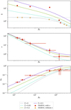Fig. 2. Dependence of model parameters: toroidal field production efficiency, αB (lower panel), reconnection efficiency, ν (middle panel), and the magnetic field gradient parameter, $\stackrel{\sim }{q}$ (upper panel) on the magnetic parameter in the disk midplane β0. Points denote values obtained from numerical simulations in SSAB16 and lines are our results from the power-law relation between αB and η (Eq. (33)) for four values of ξ.

For strongly magnetized case, simulations show that α_B ≈ η ≃ 0.3, β₀ ≃ 1 and ξ ≃ 0, which gives the reconnection efficiency parameter ν = 0. This means that the field production is efficient, the outflow is at a high rate, and dissipation by reconnection is low. On the other hand, for the weakly magnetized case, simulations result in α_B ≃ 0.02, η ≃ 0.04, β₀ ≃ 50, and due to frequent dynamo reversals, ξ ≃ 0.5. For this case, the reconnection efficiency parameter ν ≃ 50. On the other hand, SSAB16 concluded that models with ν higher than a few tend to overestimate the magnetic field gradient for weakly magnetized models and that ν = 0 describes the magnetic pressure descent more accurately for these cases (see Fig. 13 from SSAB16). This means that it would be more consistent to assume the ν parameter to have relatively low values, on the order of a few, to be in agreement with the vertical shape of the magnetic pressure.

To reduce the number of magnetic parameters to consider, we assumed a constant value of ξ and made the simplification that α_B and η are tied by a power law relation. Using Eq. (29), we recomputed α_B, which is consistent with an assumed value of ξ and η^sim and ${\beta }_0^{\text{sim}}$ taken from Tables 2 and 3 of the SSAB16 paper,

$$\begin{array}{c}\hfill {\alpha }_{\mathrm{B}}=\frac{{\eta }^{\mathrm{sim}}+\xi }{{\beta }_0^{\mathrm{sim}}+1}\end{array}$$(32)

We then performed a power-law fit and found that for ξ = 0.05 the relation that best fits the six data points is

$$\begin{array}{c}\hfill \eta =1/3{\alpha }_{\mathrm{B}}^{7/18}.\end{array}$$(33)

The dependence of the magnetic parameters on the use of these analytical formulae is plotted by lines in Fig. 2 for comparison with simulations. The figure shows that we can adopt the values of magnetic parameters, which are consistent with simulations.

The upper panel of Fig. 2 shows the magnetic pressure gradient, which is an important quantity influencing the magnetic energy release. The magnetic pressure gradient can be derived from Eq. (5) and yields

$$\begin{array}{c}\hfill q=-\frac{\mathrm{d}ln{P}_{\mathrm{mag}}}{dlnz}=2+\frac{{\alpha }_{\mathrm{B}}}{\eta }(\nu -\frac{P_{\mathrm{tot}}}{P_{\mathrm{mag}}})·\end{array}$$(34)

In the corona, when P_gas + P_rad ≪ P_mag, we can substitute P_tot/P_mag ≃ 1. The value of q is then constant, and when we express it in terms of model parameters only, we obtain a result that is compatible with Eq. (37) in BAR15:

$$\begin{array}{c}\hfill q\approx \stackrel{\sim }{q}=2+\frac{{\alpha }_{\mathrm{B}}(\nu -1)}{\eta }=\frac{2{\beta }_0}{1+{\beta }_0-\nu }·\end{array}$$(35)

With α_B remaining the only free magnetic parameter in our model, the value that we find most suitable for potentially interesting disks is α_B = 0.1. For this parameter, the radial distribution of the toroidal magnetic field at the equatorial plane B₀ and at the base of the corona B_cor (where the gas temperature achieves minimum), depending on the accretion rate and the distance from black hole, is given in Fig. 3. The magnetic field in our computations never approached values of 10⁸ G.

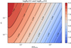Fig. 3. Toroidal magnetic field at the equatorial plane B0 and in the corona Bcor at optical depth τcor (see text for definition) in Gauss units. Logarithmic values of the magnetic field are plotted in the radius (R/Rschw) – accretion rate (ṁ) parameter plane.

3.2. Characteristics of the vertical profile

The typical structure of the disk-corona system for ṁ = 0.05 and R/R_Schw = 10 is shown in Fig. 4. The results are presented with respect to the height above the disk midplane z/H, where half of the disk thickness is given by

$$\begin{array}{c}\hfill H=\sqrt{\frac{{\int }_0^{\infty }\rho z^2\mathrm{d}z}{{\int }_0^{\infty }\rho \mathrm{d}z}}·\end{array}$$(36)

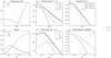Fig. 4. Vertical structure of the disk-corona system computed at the single radius R = 10 RSchw for ṁ = 0.05. The horizontal axis is the height above the disk midplane given in scale height H defined by Eq. (36). Three significant locations are marked with vertical dotted lines: the photosphere (green), the temperature minimum (dark yellow), and the thermalization depth (red). The following panels display (a) radiation and gas temperature; (b) gas, radiation, magnetic, and total pressure; (c) gas density and pressure gradients; (d) radiative energy flux, magnetic (Poynting) flux, and gas heating rate all normalized to the total accretion flux Facc; (e) net radiative cooling terms (ΛB and ΛC) and gas magnetic heating rates; and (f) electron scattering and total and effective optical depths.

Furthermore, to better present the results, we defined the total optical depth of the system according to the standard formula dτ = −κ^Pρ dz, where the electron scattering optical depth is denoted as dτ_es = −κ_esρ dz, and the density number per unit of volume is n_H = ρ/m_H.

In our model the transition in vertical structure between the disk and warm corona occurs naturally, therefore we show the location of the photosphere τ  =  2/3 and thermalization depth τ^⋆  =  1, where the seed photons originate (see Rybicki & Lightman 2008, Sect. 1.7), by the vertical lines in Fig. 4. The thermalization depth is equivalent to the effective optical depth, which in our case was computed using Planck opacities (see Sect. 2.2). We took the temperature minimum as the inner boundary of the corona, and we refer to electron scattering optical depth of the temperature minimum as τ_cor, which is also marked by a vertical line in all panels of Fig. 4.

Although the geometrical proportions and physical parameters can vary when the model input changes, we almost universally obtain a structure in which three distinct regions can be observed that directly correspond to the gas pressure structure: (i) the accretion disk, where most of the matter is located, characterized by high density near the midplane, the gas temperature that exactly follows the radiation temperature, and domination of the gas and radiation pressure over the magnetic pressure; panels a and b. (ii) The transition region, where bremsstrahlung is still an important cooling mechanism and the gas temperature is coupled to the radiation field temperature, but the magnetic pressure takes over in supporting the structure and slows the density decrease with height; panel c. (iii) The corona, where the density is low and therefore the temperature must increase with height so that the disk remains in energy equilibrium; matter is cooled mainly by the inverse Compton scattering, while the density structure is fully supported by the magnetic pressure; panels b and c. In the case presented in Fig. 4, the following regions extend within 0 ≤ z/H ≲ 3, 3 ≲ z/H ≲ 7, and 7 ≲ z/H, respectively. A noticeable increase in temperature appears in the transition region, when the warm corona starts to form due to the magnetic heating.

The overall magnetic pressure profile (see panel b) is in agreement with that obtained by BAR15, which confirms the correctness of our calculations. The density profile of the outermost coronal layers is fully shaped by pressure gradients, of which the magnetic pressure gradient is the largest (see panel c).

When we solve the vertical structure of the MSD, the magnetic energy flux F_mag needs to be considered in addition to the radiative energy flux F_rad, the latter being the only energy transport channel in a classical α-disk. Both fluxes normalized to F_acc are shown in Fig. 4d and are equal to zero in the disk midplane. In contrast to the α-disk, where the heating is mostly located near the disk midplane, we obtained a heating distribution that peaks at a few scale heights, although still below the temperature inversion point; see Fig. 4e. This behavior is mostly the effect of purely magnetic heating ℋ_mag, which depends on the magnetic pressure gradient. Heating by reconnection ℋ_rec is proportional to the magnetic pressure (rather than its gradient) and peaks around the midplane.

The total optical depth of the disk-corona system is about 10⁴. The differences between various optical depth profiles are visible in panel f of Fig. 4. For the above example, the whole corona is dominated by electron scattering, that is, τ_es = τ. The corona starts at τ_cor ∼ 10, and the total optical depth τ ∼ 20 where full thermalization occurs, for instance, τ^⋆ = 1. The corona is optically thick, which agrees with recent observations.

3.3. Thermal instability of the intermediate layer

Thermal instability in the medium can occur if under given conditions the cooling rate does not increase with temperature. The thermal balance equation then has three solutions, and if the matter is on the unstable branch, a thermal runaway or collapse occurs, following a small deviation from equilibrium. The coronal thermal instability in accretion disks has been investigated for many years (Krolik et al. 1981; Kusunose & Mineshige 1994; Nakamura & Osaki 1993; Różańska & Czerny 1996; Różańska et al. 1999), but it has never been treated in the presence of magnetic field.

Considering the static vertical structure of the accretion disk, it is reasonable to assume that any thermal collapse is an isobaric process. The condition for thermal instability reads

$$\begin{array}{c}\hfill {\mathcal{L}}_{\mathrm{rad}}\equiv {\frac{\mathrm{d}ln{\mathrm{\Lambda }}_{\mathrm{rad}}}{\mathrm{d}lnT}|}_{\delta P_{\mathrm{gas}}=0}<0.\end{array}$$(37)

When we split the cooling into Λ_B and Λ_C contributions and substitute the opacities given by Eqs. (10) and (11), we obtain

$${\frac{\text{d}{\Lambda }_{\text{B}}}{dT}|}_{\delta P_{\text{gas}}=0}=2\sigma \frac{{\kappa }_{\text{ff}}^{\text{P}}}{T}\left(11T_{\text{rad}}^4-3T^4\right),$$(38)

$${\frac{\text{d}{\Lambda }_{\text{C}}}{dT}|}_{\delta P_{\text{gas}}=0}=16\sigma \frac{{\kappa }_{\text{es}}\rho }{T}\frac{k{T}_{\text{rad}}^5}{m_e{c}^2}\cdot$$(39)

Depending on the contributions from these two terms, we distinguish tree cases: i when Λ_B ≪ Λ_C, the solution is always thermally stable because Eq. (39) has positive sign, ii when Λ_B ≫ Λ_C, instability occurs for

$$\begin{array}{c}\hfill T\ge \sqrt[4]{\frac{11}{3}}{T}_{\mathrm{rad}}\approx 1.38T_{\mathrm{rad}},\end{array}$$(40)

and finally, iii when Λ_B ≈ Λ_C and T >  T_rad, radiative heating by bremsstrahlung is negligible, and the criterion for instability reads

$$\begin{array}{c}\hfill {\rho }^{2}T\ge {\left[\frac{8}{3}\frac{{\kappa }_{\mathrm{es}}}{{\kappa }_{\mathrm{ff},0}^{\mathrm{P}}}\frac{k{T}_{\mathrm{rad}}^5}{m_e{c}^2}\right]}^2\approx 4.30\times {10}^{-9}{\left(\frac{T_{\mathrm{rad}}}{{10}^6\mathrm{K}}\right)}^{10}·\end{array}$$(41)

In the isobaric regime, when δP_gas = 0 or ρT = const., this defines the upper limit for the temperature for which thermal instability occurs. The transition between these regimes ii and iii occurs for the density

$$\begin{array}{c}\hfill \rho =\frac{8}{3}\sqrt[8]{\frac{3}{11}}\frac{{\kappa }_{\mathrm{es}}}{{\kappa }_{\mathrm{ff},0}^{\mathrm{P}}}\frac{k{T}_{\mathrm{rad}}^{9/2}}{m_e{c}^2}\approx 5.58\times {10}^{-35}{T}_{\mathrm{rad}}^{9/2}.\end{array}$$(42)

In order to show the transition between stable and unstable corona, the net cooling function in MSD for three slightly varying accretion rates 0.35, 0.50, and 0.72 is presented in Fig. 5 for the radiation temperature T_rad = 10⁶K. The three models vary mainly by the shift in density; the highest density corresponds to the lowest accretion rate.

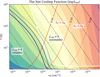Fig. 5. Logarithm of the net cooling rate Λrad (Eq. (17)), plotted in the nH – T parameter plane ranging from blue (low rate) to red (high rate). The points of constant pressure are connected with black dash-dotted lines. The red dotted contours show the contribution of the Compton cooling to the total cooling. The solid white line shows where the cooling function is constant in isobaric perturbation, and separates the area of unstable solutions where the gradient of the cooling function ℒrad <  0. Dark blue lines of increasing width represent the vertical structure for three accretion rates 0.035, 0.050, and 0.072.

Each model starts at the disk midplane where T ≈ T_rad, and only when the transition to the corona starts does the gas temperature diverge from the radiation temperature. When the density is higher than that given by Eq. (42), the model will inevitably enter the zone defined by Eq. (40). Otherwise, for hotter disks, the contribution of Compton cooling will yield at least half of the total cooling, and the model might graze the instability boundary defined by Eq. (41) but never exceed it. This means that all but the Compton-dominated disks will be affected by thermal instability of the transition region. The only stable solution is possible for relatively rare disks for the low cooling rate, that is, the left-hand side of the white thick solid line.

The same three models are shown Fig. 6. In order to identify all thermal equilibrium solutions for each height above the disk midplane, the fraction of Compton cooling, the energy balance, and the cooling function gradient ℒ_rad are shown depending on the gas temperature T while maintaining constant gas pressure. For the hottest model (highest accretion rate), there is an unambiguous solution in each point. This changes when the temperature decreases: although the main continuous solution is still stable (compared to Fig. 5), two cooler solutions appear. The middle solution lies within the unstable zone (pink area in the third column), but the coldest solution is stable. This means that because this area is dominated by magnetic pressure, an abrupt density change would not greatly affect the hydrostatic equilibrium and the existence of two-phase matter is possible. Finally, for the lowest accretion rate (upper panels of Fig. 6), no numerically consistent stable solution exists. We expect that matter in this region would remain cold, but above the unstable region, a corona might still form. This corona would be hot and optically thin, and in the example we discussed, the transition would occur at about z/H ∼ 20.

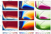Fig. 6. Onset of thermal instability in a low-temperature disk, ṁ = 0.035 shown in the top panels, and its stabilization with the increase of the temperature, ṁ = 0.05 and 0.072 shown in the middle and bottom panels. Other disk parameters are as given in Sect. 3.1. In each panel the vertical axis represents the possible gas temperature T assuming constant gas pressure (δPgas = 0), and the horizontal axis is the height above the disk midplane given in scale height H (Eq. (36)). The possible solutions that satisfy the radiative energy balance are shown with thick black contours, while the solution obtained from our numerical computations is additionally marked with light gray dots. A thinner gray line is used to show the radiation temperature, Trad. Color maps in the first panels column show the contribution from Compton scattering to the total cooling. In the second column, the overall heating-cooling balance is shown: the yellow-orange areas are where the heating dominates cooling, and blue areas show where the cooling rate exceeds the heating. The third column presents the stability diagnostic, i.e., the cooling function gradient ℒrad (Eq. (37)), with green areas marking the stable regions and violet areas the unstable regions. Two limit solutions according to Eqs. (40) and (41) are plotted with orange lines (dash-dotted and dashed, respectively) and show excellent agreement with the numerical solution. Additionally, the content of neighboring plots (from right panels to the middle, and from middle to the left) are superimposed as thin contours for the sake of clarity.

Equations (40) and (41) define the lower and upper limits for the temperature that allows the occurrence of thermal instability. This is clearly shown in Fig. 5, as each isobaric contour slices the instability boundary in exactly two points. These solutions are also plotted in Fig. 6 with orange lines. They indeed suffice to describe the instability in most of the vertical structure of the disk.

3.4. Local properties of the corona

The disk-corona transition at the given radius depends on the value of the local temperature and density. We present here the evolution of the selected disk parameters with an accretion rate and magnetization state with the aim to demonstrate better how the warm corona can arise at radius R = 10 R_Schw. For this purpose we define here two additional quantities related to the radiation pressure because the radiation energy is the main observable of the accretion disk-corona systems. The first such quantity is the so-called radiation efficiency, that is, the ratio of the radiation flux to the total flux that is dissipated locally at a certain point of the vertical structure due to magnetic field reconnection F_rad/F_acc, while the second quantity is the ionization parameter Ξ (Krolik et al. 1981), which is defined as

$$\begin{array}{c}\hfill \mathrm{\Xi }=\frac{P_{\mathrm{rad}}}{P_{\mathrm{gas}}}·\end{array}$$(43)

In Figs. 7 and 8 we show the structure of the temperature, the magnetic field gradient, the radiation efficiency, the cooling function gradient, the contribution of Compton cooling to the total cooling, and the ionization parameter in panels a to f, respectively. For all cases of the accretion rate we achieve a hot outermost layer at the top of the inner accretion disk.

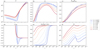Fig. 7. Vertical structure of the disk-corona models computed at R = 10 RSchw for different values of the accretion rate (ṁ), plotted against the total optical depth τ. The panels show (a) the gas temperature, (b) the gradient of the magnetic pressure (Eq. (34)), (c) the radiative energy flux normalized to the total accretion flux Facc, (d) the cooling function gradient (Eq. (37)), (e) the contribution of Compton cooling to the total cooling, and (f) the ionization parameter Ξ (Eq. (43)).

Fig. 8. Same as in Fig. 7, but for different values of the magnetic parameter αB.

The temperature of the corona is very stable with respect to the accretion rate, but the optical depth for which the disk-corona transition occurs increases with accretion rate and reaches the value of ≈10 for ṁ = 0.71. In contrast, the accretion rate determines the density of the disk, and consequently, the value of the magnetic pressure gradient that saturates in the disk at the highest value for the lowest accretion. At the point of disk-corona transition, the magnetic pressure slightly decreases, but the rate of the radiative energy release is roughly the same, see panel c. We conclude that the primary factors causing the optical depth of the corona to vary are the changes in disk temperature (and the transition region, consequently).

Panel e partly explains this behavior: for lower accretion rates, cooling in the disk is dominated by bremsstrahlung, which switches off at around τ ∼ 1, causing an abrupt temperature gradient in the corona boundary. At the same time, the cooling function gradient also becomes negative for these cases (panel d). We conclude here that this contribution from bremsstrahlung also causes the formation of an unstable region, as discussed in Sect. 3.3. For higher accretion rates, the contribution from bremsstrahlung is not that significant, and the transition from the disk to the corona is almost seamless. The ionization parameter presented in panel f does not indicate a thermally unstable region. It shows the inversion with optical depth, which is shallower for Compton-dominated cases (high accretion rate). Finally, Ξ is larger for hotter and rarer disks.

The changes in the corona are much more dramatic when the dependence on the magnetic field is examined, as shown in Fig. 8. Panel a shows that corona optical depth and temperature are radically different for weak and strong magnetic fields. For the weak field, the disk is much hotter and the radiation flux almost saturates to its maximum value well inside the disk (panel c), blue line, in contrast to the strong field case, where the disk is much colder, and more than half of the thermal energy is released in the corona above τ = 1 (panel c), red line. For the corona the temperature behavior is exactly opposite.

When magnetic pressure play a dominant role in the corona, it changes as $P_{\mathrm{mag}}\propto z^{-\stackrel{\sim }{q}}$, the density changes as $\rho \propto z^{-(\stackrel{\sim }{q}+1)}$, and the heating rate changes as $\mathcal{H}\propto z^{-\stackrel{\sim }{q}}$. High values of q mean a very steep decline in magnetic field strength and gas heating rate, which in turn means that most of the energy will be dissipated within the disk, and the corona will be weak. This behavior is nicely demonstrated in panel b of Fig. 8. A stronger magnetic field adds to the effective disk cooling and consequently results in the appearance of thermal instability in disk-corona transition (panel d). Despite large temperature differences, Ξ within the disk remains almost constant (panel e), while in the corona it decreases with magnetization even if the coronal temperature is higher.

3.5. Global properties of the corona

To analyze the global behavior of our model within the parameter space, we define below several diagnostic quantities as proxies for various properties of the disk-corona system. We intended to select these quantities so that they can be compared to observables. The maps in Figs. 9–11 present these diagnostics depending on distance from the black hole R/R_schw, accretion rate ṁ, and α_B parameter.

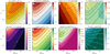Fig. 9. Properties of the corona on the radius (R/Rschw) – accretion rate (ṁ) parameter plane. All models are calculated for MBH = 10M⊙, αB = 0.1, and ξ = 0.05. The panels display (a) the average temperature of the corona (Eq. (44)) in keV (colors) and τcor (contours); (b) the ionization parameter Ξ (colors) and magnetic β parameter (contours), both at the disk midplane; (c) the number density at τ = 2/3 (colors) and the total column density Σ in g cm2 (contours); (d) the fraction of radiative energy produced by the corona f (Eq. (45), colors), the maximum value of the magnetic field gradient q (Eq. (35), contours); (e) the y parameter of the warm corona (Eq. (46)), computed up to the thermalization layer τ⋆ = 1 (colors) and to τcor (contours); the (f) photon destruction probability $ϵ={\kappa }_{\mathrm{ff}}^{\mathrm{P}}/{\kappa }^{\mathrm{P}}$ (colors) and electron scattering optical depth (τes) (contours) at the thermalization layer; (g) the minimum value of ℒrad (Eq. (37)) throughout the disk height (colors), here, green areas are stable disks, and magenta areas indicate thermal instability in the corona, the gray dotted line corresponds to ℒrad = 0, and the ionization parameter Ξ at the corona base (contours); and (h) the radiative energy flux normalized to the total accretion flux (colors), and the disk scale ratio H/R (contours).

Similarly to RMB15, and opposite to most models, our corona does not have a constant temperature, but changes with the optical depth, reaching temperature minimum at τ_cor. From X-ray spectral fitting we measure some averaged temperature of the warm medium cooled by Comptonization, therefore it is useful to define the average temperature of the corona as

$$\begin{array}{c}\hfill T_{\mathrm{avg}}={\tau }^{-1}{\displaystyle {\int }_0^{{\tau }_{\mathrm{cor}}}T\mathrm{d}{\tau }^{\prime }}\end{array}$$(44)

with the aim to compare it with observations. Both quantities T_avg and τ_cor are shown in each panel a of three maps. A warm optically thick corona tends to form above the inner strongly magnetized disk of high accretion rate.

Analogously to Haardt & Maraschi (1991), we denote the fraction of thermal energy released in the corona (versus total thermal energy) as

$$\begin{array}{c}\hfill f=\frac{F_{\mathrm{rad}}^{\mathrm{cor}}}{F_{\mathrm{rad}}^{\mathrm{tot}}}=1-\frac{F_{\mathrm{rad}}^{\mathrm{disk}}}{F_{\mathrm{rad}}^{\mathrm{tot}}}·\end{array}$$(45)

f = 0 corresponds to the passive corona, and f = 1 corresponds to passive disk. This parameter is shown in panel d and is tightly correlated with the magnetic field gradient q (Eq. (35)), plotted with contours. Because f is dependent only on magnetic parameters, we suggest that a strong magnetic field is required to obtain the high values of f that are reported by observations. Although we never approach f ≈ 1 and therefore cannot reproduce the passive-disk scenario discussed by Petrucci et al. (2013, 2018) for the case of AGN, we show that up to half of the total accretion energy can be dissipated in the corona.

Another useful quantity is the Compton y parameter, which can also be determined from observations. To derive the y value for our corona, we used the following definition, which incorporates an additional term that accounts for optically thick medium:

$$\begin{array}{c}\hfill y_{\mathrm{avg}}={\displaystyle {\int }_0^{{\tau }_{\mathrm{es}}}\frac{4k(T-T_{\mathrm{rad}})}{m_e{c}^2}(1+2{\tau }_{\mathrm{es}}^{\prime })\mathrm{d}{\tau }_{\mathrm{es}}^{\prime }.}\end{array}$$(46)

The value of this parameter is shown in panels e of Figs. 9–11 and can range between 0 and 0.5. This is consistent with the values obtained from observations of X-ray binaries: y ≈ 0.3 (Życki et al. 2001), y ≈ 0.4 (Goad et al. 2006), and up to y ∼ 1 (Zhang et al. 2000).

All these quantities (τ_cor, T_avg, f, and y_avg) positively correlate both the with magnetic field strength and with the released accretion power. This means that the most prominent corona would be observed in the case of a high accretion rate and a strong field. However, above some threshold of disk magnetization (around α_B = 0.2, which corresponds to q ≈ 1.3), the trend reverses, and magnetic flux escapes without releasing all of its energy into radiation, as is shown in panel i of Figs. 10 and 11.

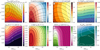Fig. 10. Same as in Fig. 9, but on the radius (R/Rschw) – toroidal field production parameter (αB) plane.

Fig. 11. Same as Fig. 9, but on toroidal field production parameter (αB) – accretion rate (ṁ) plane.

In the case of GBHBs, where the disk temperatures are generally high, the optical depth of the corona τ_cor is not usually limited by a thermalization layer τ^⋆  =  1 because the medium is strongly scattering dominated, as presented in panel f of Fig. 9. The electron-scattering optical depth of this layer is usually ten times higher than τ_cor for the parameters considered here. Photons become thermalized due to high free-free absorption, as we show in comparison to the total Planck opacity in the same panel.

Even if the corona might exist as a solution, thermal instability will occur in many cases, as discussed in Sects. 3.3 and 3.4. Panels g of Figs. 10 and 11 show the stability of the warm corona solutions. The dependence on accretion power is very abrupt and almost switch-like: if the matter becomes too cold or too dense and the contribution of bremsstrahlung cooling accordingly increases, thermal instability occurs, and the corona cannot exist as a stable uniform layer (magenta regions). The same effect is obtained when the magnetic field strength increases and the disk becomes colder (compare with Fig. 8), but the transition is less sensitive and more gradual. The instability appears mostly in cold disk regions, that is, for a low accretion rate and a high magnetic field, and will remove only the optically thick skin when bremsstrahlung contribution is significant, and will most likely not affect the optically thin hot corona, which will still be present, even if its optical depth may vary with radius and accretion rate. This result, particularly the existence of the corona only around the zone of the maximum energy dissipation rate (around R/R_schw = 10) is consistent with Kusunose & Mineshige (1994).

The disk thickness d = H/R, where H is defined by Eq. (36), is shown in panels i of the figure maps. It ranges between 10⁻³ and 10⁻¹, which means that we still remain in thin-disk regime, consistent with the assumption. It is important to note that the disk thickness changes mostly with the accretion rate. The increase in magnetic field strength does not inflate the disk (Fig. 11i) when the radiative pressure is included, as the fraction of energy that is dissipated within the disk decreases (panel d), and a disk core that is supported by radiative pressure (as in a classical α-disk) is not present, as shown by the radiative to gas pressure ratio Ξ in panel b. Similarly, the total column density Σ, shown by contours in panels c, is decreased because the magnetic fields take over the role of supporting the disk structure.

4. Discussion and conclusions

A disk with an optically thick corona is a frequently used satisfactory representation of the accretion sources in the soft state, and we self-consistently modeled this structure here, based on first principles. Using a semi-analytical static model of the magnetically supported disk (MSD) with radiation, we developed a new relaxation numerical code to calculate the disk-corona transition. The relaxation method designed by us and described in Appendix A is general (Henyey et al. 1964) and solves any set of linear differential equations with assumed boundary conditions. For the case of an accretion disk with a corona, we solved a set of five equations, four of which are differential and one is algebraic, with four boundary conditions (Sect. 2.3).

Our code fully solves the vertical structure, taking into account that part of the magnetic energy generated in the MRI process is converted into radiation and can be dissipated in the warm Compton-cooled corona. The remaining part of the magnetic flux is channeled into a toroidal magnetic field and escapes from the system, as introduced by BAR15. The original model proposed by BAR15 included no energy balance checking or radiative transfer, however, which allowed reducing the model to dimensionless equations. In this paper, we combined the MSD of these authors with solving the radiation transfer through the gray atmosphere in radiative and hydrostatic equilibrium. Additional mean opacities due to free-free absorption are taken into account.

In case of GBHBs with a black hole of stellar mass, we were able to reproduce both an optically thick and thin corona, which is commonly detectable in observations of accreting sources. In contrast to our previous paper (RMB15), where coronal heating was artificially assumed and kept constant with height, here we obtained a self-consistent transition through all three layers: (i) a deep accretion disk up to a few scale heights that is dense and fully thermalized, (ii) a warm corona, where magnetic pressure slows the density decrease and the temperature slowly starts to increase, and (iii) a hot Corona where the density is low. Compton cooling is fully taken into account in all layers, but it strives against free-free cooling depending on the local physical gas conditions (see panel e in Figs. 7 and 8).

The base of the corona at temperature minimum τ_cor may reach 10 electron scattering optical depths, while the thermalization zone can be even 60 times τ_es (panels a and f in Figs. 9–11). This agrees with some observations of a warm Compton-thick corona (Zhang et al. 2000; Życki et al. 2001). The temperature, optical depth, and energetic output of the corona are dependent on distance from the black hole, accretion rate, and toroidal magnetic field strength. A high accretion rate and a strong toroidal field are favorable conditions for the development of a warm ∼5 keV and optically thick τ_cor ∼ 11 corona, as shown in the upper left corner of panel a in Fig. 11.

The magnetic field strength, β₀, seems to have a leading role in regulating the formation of the corona because the energy is stored very efficiently in the poloidal magnetic field near the equatorial plane, and the Poynting flux, F_mag, quickly increases, reaching its maximum value at approximately z/H ∼ 2 for the case presented in Fig. 4, panel d. At this point, the magnetic energy stored in the outflowing field is gradually released by heating the gas. Farther out in the atmosphere, this heating rate exceeds the magnetic energy gain from the toroidal field production (MRI). Asymptotically, the Poynting flux will fully convert into the radiation flux, but practically, this convergence may be very slow in some cases (particularly for strongly magnetized disks, where the magnetic pressure declines slowly with height). Therefore, the magnetic pressure gradient q (Eq. (34)) is an important quantity that influences the release of magnetic energy and in consequence, the formation of the corona (see panel b) in Figs. 7 and 8. A stronger toroidal field, that is, a lower β₀, implies a milder gradient and more accretion energy that is transported from the disk to the atmosphere by Poynting flux. This is nicely demonstrated in panel b of Fig. 11, where the values of β₀ are lowest, and where the warm corona has the highest optical thickness (panel a) of the same figure. On the other hand, the radiative flux F_rad will never saturate asymptotically to a constant value for q ≤ 1 (see panels d) and i in Fig. 11.

However, an optically thick corona may be subject to local thermal instability caused by contribution of free-free opacity in the transition layer. These instabilities have been problematic in radiative transfer computations of accretion disk atmospheres of AGN for decades (Krolik & Kriss 1995; Nayakshin et al. 2000; Różańska et al. 2002, 2015). We were expecting that in case of hotter disks around black holes of stellar mass those instabilities would be absent, and in addition, magnetic heating might remove them. Our results show the opposite, however: a stronger field expands in the corona vertically and at the same time prevents formation of a very hot disk that is supported by radiation pressure, which might be sensitive to thermal instabilities. When this happens, two outcomes are possible: the sharp transition between cold and hot phase will be smoothed out by thermal conduction and form a relatively plain and regular atmosphere (Różańska 1999), or prominence-like clumps of dense matter will form, and will coexist at the same level with hot medium, similar to lower solar corona. The clumps could condense or simply emerge from the disk, pulled by magnetic field buoyancy (Fig. 1 in Jiang et al. 2014). Given the violent and turbulent nature of an assumed engine that powers the disk (MRI), the clumpy two-phase medium interpretation seems more likely, but also poses a huge challenge for spectrum modeling. Variations of this scenario that often consider not only a corona but an entire disk that is clumpy have been discussed in the literature (Schnittman & Krolik 2010; Yang et al. 2015; Wu et al. 2016). Regardless of the interpretation, we show that thermal instability occurs in very many cases, even though GBHB disks are hot and dense and not as prone to it as AGN disks.

Although thermal instability affects the very same transition region that is responsible for producing optically thick corona, our model places constraints on the parameters for which a warm or hot corona can exist. For this purpose, we drew the radial extension of the corona base determined by the usual temperature minimum when no thermal instability is present, or by the temperature of the upper stable branch where thermal instability starts to developed (the cross point in the upper panels of Fig. 6) with the black dotted line in Fig. 12. The gas density, average temperature, and the radial profiles of the Compton parameter at selected optical depths for three accretion rates are shown in Fig. 12.

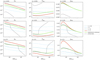Fig. 12. Radial profiles of selected quantities: gas density ρ [cm−3], average temperature Tavg [K], and average Compton yavg (Eq. (46)), measured at different depths in the disk atmosphere. Values at τ = 0.1, τ = 1, and τ = 10 are shown by dashed blue lines, at temperature minimum (τcor) by the green line, at thermalization depth by the red line, and at the corona base (determined by temperature minimum or thermal instability in case it is developed) with the black dotted line.

When the accretion rate is low, thermal instability arises at each distance from the black hole and only a hot corona appears, which is four orders of magnitude less dense than the disk atmosphere (three upper panels of Fig. 12). A corona like this would be optically thin, and the transition between disk and corona occurs at about z/H ∼ 20, as demonstrated in the upper panels of Fig. 6. For ṁ = 0.05, a warm stable corona can form up to R ∼ 10 R_Schw, and this corona is dense and optically thick, reaching at the base almost τ_es ∼ 10 (three middle panels of Fig. 12). Nevertheless, farther out from the black hole, thermal instability arises and a stable corona is again very hot and rare. Such a hot and rare outer corona dissipates only about 1% of the local energy and cannot be associated with the usual hard X-ray corona observed in accreting sources. Finally, for a high accretion rate ṁ = 0.5, the radial extent of the warm corona is the largest ∼60 R_Schw and optical depth τ_es = 10. Thermal instability and a hot stable corona appear farther away from the black hole. Our results strongly indicate that a warm optically thick corona tends to develop in the innermost disk regions, while the outer disk is covered only by a rare hot corona. Furthermore, a warm corona is more radially extended for disks of high accretion rates. This feature explains why we see soft X-ray excess only in the most luminous accreting sources.

Our model predicts a corona formation that is adjusted self-consistently by model parameters, therefore it places constraints on several quantities that can be directly compared with observations. The fist straightforward outcome is that the value of the temperature T_avg is in the range from 0.1–10 keV. The second constrained parameter is the density of the warm corona, which arises from the dense disk atmosphere. The predicted density from our model is about 10^{16 − 20} cm⁻³. This density is very high, but it agrees with the density of the ionized outflow in accreting black holes that was determined from observations by Miller et al. (2014). Our model supports the scenario that eventually, a disk wind can arise from the upper dense layers of a magnetically driven accretion disk atmosphere.

The most important observable is the ratio of the thermal energy that is released in the corona f in comparison to the total energy that is generated in the system. This ratio is always higher than zero because we computed a Compton-cooled atmosphere, which is characterized by typical temperature inversion with increasing optical depth (Różańska et al. 2011). In the frame of our model, we showed that up to half of the total accretion energy can be dissipated in the corona in case of GBHBs (up to f = 0.75 for the highest value of α_B), therefore we are not able to reproduce the passive-disk scenario discussed by Petrucci et al. (2013, 2018) for the case of AGN. This is a natural consequence of our assumed heating mechanism, which can transport a large portion of energy to the corona, but requires very effective magnetic coupling with gas down to the equatorial plane. The value of the Compton parameter averaged over the optical depth of the warm corona we determined with our model is consistent with the values determined from X-ray observations of several GBHBs: y ≈ 0.3 (Życki et al. 2001), y ≈ 0.4 (Goad et al. 2006), up to y ∼ 1 (Zhang et al. 2000).

One of the main postulates of the BAR15 model is that it can explain the spectral state transition of the X-ray binary that is observed in many sources (e.g., Yamada et al. 2013) by a smooth transition from the soft to hard state by introducing an intermediate dead zone between the disk and the coronal accretion flow. They used the condition for MRI shutoff when the gas energy is not high enough to sustain the dynamo (Pessah & Psaltis 2005). In our model, we considered only one zone where MRI is always operating. We suggest here that the spectral state transition should occur depending on the strength and radial extension of the warm optically thick corona rather than the full MRI shutoff. In the frame of our model we did not consider the transition from optically thick disk to inner advection-dominated accretion flow.

As discussed in BAR15 and SSAB16, one of the key features of MSDs is that they require a strong global poloidal magnetic field for the magnetic dynamo to operate and generate the toroidal field that supports the disk. In case of our typical model α_B = 0.1, the toroidal magnetic field in the equatorial plane and at the base of corona typically is about 10⁸ G in the inner disk region and of 10⁵ G for radii above 70 R_Schw. These values are lower than those detected in pulsars, but they fully agree with the prediction for the poloidal magnetic filed value that is required for the jet-launching mechanism.

Studies suggest that a poloidal magnetic fields is important in jet-launching mechanisms (see also Beckwith et al. 2009; McKinney et al. 2012; Liska et al. 2018). Zhang et al. (2000) noted that in both objects where an optically thick corona was observed, jets were also present. Our study shows that the most prominent warm corona will occur in a state when the dynamo is very effective (high α_B) and the contribution of the magnetic field to the disk structure is high (low β₀). On the other hand, no jet was observed in Mrk 509 (Petrucci et al. 2013). Nevertheless, the case of AGN will be presented in a forthcoming paper.

Acknowledgments

We thank Bożena Czerny for all comments and helpful discussion. This research was supported by Polish National Science Center grants No. 2015/17/B/ST9/03422 and 2015/18/M/ST9/00541.

References

Appendix A: Numerical procedure

The solution of the set of five equations with four boundary conditions described in the previous sections allows determining the density ρ, gas temperature T_gas, radiation pressure P_rad, radiative flux F_rad, and magnetic pressure P_mag at each point of the vertical profile. The requirement of satisfying four boundary conditions, two on each side of the computational interval, requires multiple iterations when shooting methods such as a Runge-Kutta scheme are used. Moreover, the equations are highly nonlinear, and keeping the integration error low requires a high number of grid points (up to 10⁵), even using a fourth-order Runge-Kutta scheme. Although the computation time using a shooting method is still less than a few minutes, it becomes a problem when the global behavior over the parameter space is investigated, which requires computing thousands of models for different disk and magnetic parameters. Therefore, to solve this issue, we developed a variant of the relaxation method that was originally described by Henyey et al. (1964) for stellar evolution problems.

The relaxation methods are iterative, when iterations are made for the functions defined in the whole argument space. In the first step, some approximate solution for the functions, which might be close to the exact solution, is needed. Then by applying the procedure described below, the correction to the entire profile is obtained and added to the original solution. Because we have many strongly nonlinear terms in our equations while the method is intrinsically linear, we applied a reduction factor for these corrections in the first few iterations to avoid overshooting. The new solution was then used as input to the next step and the iteration continued until the mean relative value of the obtained correction fell below 10⁻⁷, which we consider a convergence criterion.

To apply the relaxation method to our problem, define a grid of N points, in each we have five physical quantities. We introduce the following notation: the quantity j = 1…5 in point i = 1…N is denoted $X_i^j$. We can also represent it as a vector with five components:

$$\begin{array}{c}\hfill {\overrightarrow{X}}_i\equiv [{\rho }_i,T_i^{\mathrm{gas}},T_i^{\mathrm{rad}},F_i^{\mathrm{rad}},P_i^{\mathrm{mag}}].\end{array}$$(A.1)

Then we discretize the set of all five equations together with the boundary conditions. For nondifferential equations (balance equation and boundary conditions), we evaluate them at the respective grid points, that is, $X^j(z)\to X_i^j$. For all four differential equations we replace quantities with midpoint values and their spatial derivatives with finite differences. As they are evaluated at midpoints, there are only N − 1 terms,

$$\begin{array}{cc}\hfill X^j(z)& \to \frac{X_i^j+X_{i+1}^j}{2}\equiv X_{i+1/2}^j,\hfill \end{array}$$(A.2)

$$\begin{array}{cc}\hfill {\frac{d{X}^j}{\mathrm{d}z}|}_z& \to \frac{X_{i+1}^j-X_i^j}{z_{i+1}-z_i}\equiv Y_{i+1/2}^j.\hfill \end{array}$$(A.3)

The core of the problem is to perturb the entire profile to obtain a new one that is closer to the solution. Using the chain rule, we can express the computed profile in terms of perturbations to actual physical quantities:

$$\begin{array}{c}\hfill \delta A_i^k={\displaystyle \sum _{j=1}^5\sum _{l=1}^N\frac{\partial A_i^k}{\partial X_l^j}\delta X_l^j=-A_i^k,}\end{array}$$(A.4)

where i = 1…N − 1 and k = 1…5. Most of the terms in this sum are zero because equations evaluated at point i depend only on quantities in points i and i + 1, thus l ∈ {i, i + 1}. The goal of the relaxation method is to transform all equations where $A_i^k=0$, which means that each of the equations k = 1…5 is satisfied in each point i = 1…N. However, having started from some initial guess, this is more likely not true, and the remainder $A_i^k\ne 0$.

Analogically, we do the same for boundary conditions. When we denote the remaining lower boundary conditions as L and upper boundary conditions as U, the expansions in terms of perturbations with respect to variables yield

$$\begin{array}{cc}\hfill \delta L^k& ={\displaystyle \sum _{j=1}^5\frac{\partial L^k}{\partial X_1^j}\delta X_1^j=-L^k\text{where}k=1,2,}\hfill \end{array}$$(A.5)

$$\begin{array}{cc}\hfill \delta U^k& ={\displaystyle \sum _{j=1}^5\frac{\partial U^k}{\partial X_N^j}\delta X_N^j=-U^k\text{where}k=1,2.}\hfill \end{array}$$(A.6)

At this point we have a mathematically well-defined problem: we must solve Eqs. (A.4)–(A.6) to obtain the profile corrections $\delta X_{1\dots N}^{1\dots 5}$. We can express it as the perturbation vector δX, remainder vector R and Jacobian matrix M:

$$\begin{array}{c}\hfill \mathbf{M}·\delta \mathit{X}=-\mathit{R}.\end{array}$$(A.7)

We arrange our five variables and five equations into a vector using the following layout:

$$\begin{array}{cc}& X_{5i-5+j}=X_i^j\text{where}j=1\dots 5\text{and}i=1\dots N,\hfill \end{array}$$(A.8)

$$\begin{array}{cc}& R_k=L^k\text{where}k=1,2,\hfill \end{array}$$(A.9)

$$\begin{array}{cc}& R_{5i-3+k}=A_i^k\text{where}k=1\dots 5\text{and}i=1\dots N,\hfill \end{array}$$(A.10)

$$\begin{array}{cc}& R_{5N-2+k}=U^k\text{where}k=1,2.\hfill \end{array}$$(A.11)

Now the remaining issue is to fill the matrix accordingly. For linear equations, to evaluate all nonzero matrix terms for i = 1…N, j = 1…5, k = 5 and l = i, we directly use the formula

$$\begin{array}{c}\hfill M_{\mathit{pq}}=\frac{\partial A_i^k}{\partial X_l^j},\text{where}\begin{array}{c}p=5i-3+k\hfill \\ q=5l-5+j.\hfill \end{array}\end{array}$$(A.12)

For differential equations, each point depends on two consecutive points, and we evaluate these terms for i = 1…N − 1, j = 1…5, k = 1…4 and l ∈ {i, i + 1} using the chain rule:

$$\begin{array}{cc}& \frac{\partial A_i^k}{\partial X_i^j}=\frac{\partial X_{i+1/2}^j}{\partial X_i^j}\frac{\partial A_i^k}{\partial X_{i+1/2}^j}+\frac{\partial Y_{i+1/2}^j}{\partial X_i^j}\frac{\partial A_i^k}{\partial Y_{i+1/2}^j}\hfill \end{array}$$(A.13)

$$\begin{array}{cc}& =\frac{1}{2}\frac{\partial A_i^k}{\partial X_{i+1/2}^j}-\frac{1}{z_{i+1}-z_i}\frac{\partial A_i^k}{\partial Y_{i+1/2}^j},\hfill \end{array}$$(A.14)

$$\begin{array}{cc}& \frac{\partial A_i^k}{\partial X_{i+1}^j}=\frac{\partial X_{i+1/2}^j}{\partial X_{i+1}^j}\frac{\partial A_i^k}{\partial X_{i+1/2}^j}+\frac{\partial Y_{i+1/2}^j}{\partial X_{i+1}^j}\frac{\partial A_i^k}{\partial Y_{i+1/2}^j}\hfill \end{array}$$(A.15)

$$\begin{array}{cc}& =\frac{1}{2}\frac{\partial A_i^k}{\partial X_{i+1/2}^j}+\frac{1}{z_{i+1}-z_i}\frac{\partial A_i^k}{\partial Y_{i+1/2}^j}·\hfill \end{array}$$(A.16)

Finally, for boundary conditions, we evaluate the matrix coefficients at lower (L) and upper (U) boundary as

$$\begin{array}{cc}& M_{\mathit{kj}}=\frac{\partial L^k}{\partial X_1^j}\text{where}k=1,2,\hfill \end{array}$$(A.17)

$$\begin{array}{cc}& M_{\mathit{pq}}=\frac{\partial U^k}{\partial X_N^j}\text{where}\begin{array}{c}k=1,2\hfill \\ p=5N-2+k\hfill \\ q=5N-5+j.\hfill \end{array}\hfill \end{array}$$(A.18)

The relaxation method provides excellent precision even for very few computational points because the method adjusts the entire profile at once, allowing us to investigate even marginally stable cases. The method is also clearly expandable for higher-order derivatives.

Its major disadvantage is the requirement that the partial derivatives of the left-hand sides of all equations (and boundary conditions) need to be evaluated with respect to all variables and their spatial derivatives. This makes the code very difficult to modify and error prone. We solved this problem using a symbolic computation techniques within the sympy framework (Meurer et al. 2017), which also allowed us to generate ready-to-compile procedures to evaluate the matrix coefficients that we included in our code, which is written in Fortran 2008. We then solved the system of linear equations using the DGBSV procedure from LAPACK (Anderson et al. 1990) and obtained corrections to all five variables at each point. This method is very fast and allows us to obtain a precise solution in less than half a second on a typical desktop computer.

All Figures

Fig. 1. Schematic illustration of a slice through the disk plane (only one side is shown due to symmetry). The black hole is shown as the circle on the left. The gray area represents the optically thick and geometrically thin disk where most of the accreting mass is located. The warm corona that covers the disk, in which the magnetic energy is released as radiation, is marked in orange. Magnetic and radiative energy flux are represented by blue and red arrows, respectively. The part of the corona that might collapse as a result of thermal instability is shown in magenta. The inner optically thin and geometrically thick hot flow that we did not consider is drawn in yellow for completion.

In the text

Fig. 2. Dependence of model parameters: toroidal field production efficiency, αB (lower panel), reconnection efficiency, ν (middle panel), and the magnetic field gradient parameter, $\stackrel{\sim }{q}$ (upper panel) on the magnetic parameter in the disk midplane β0. Points denote values obtained from numerical simulations in SSAB16 and lines are our results from the power-law relation between αB and η (Eq. (33)) for four values of ξ.

In the text

	Fig. 3. Toroidal magnetic field at the equatorial plane B0 and in the corona Bcor at optical depth τcor (see text for definition) in Gauss units. Logarithmic values of the magnetic field are plotted in the radius (R/Rschw) – accretion rate (ṁ) parameter plane.
In the text

Fig. 4. Vertical structure of the disk-corona system computed at the single radius R = 10 RSchw for ṁ = 0.05. The horizontal axis is the height above the disk midplane given in scale height H defined by Eq. (36). Three significant locations are marked with vertical dotted lines: the photosphere (green), the temperature minimum (dark yellow), and the thermalization depth (red). The following panels display (a) radiation and gas temperature; (b) gas, radiation, magnetic, and total pressure; (c) gas density and pressure gradients; (d) radiative energy flux, magnetic (Poynting) flux, and gas heating rate all normalized to the total accretion flux Facc; (e) net radiative cooling terms (ΛB and ΛC) and gas magnetic heating rates; and (f) electron scattering and total and effective optical depths.

In the text

Fig. 5. Logarithm of the net cooling rate Λrad (Eq. (17)), plotted in the nH – T parameter plane ranging from blue (low rate) to red (high rate). The points of constant pressure are connected with black dash-dotted lines. The red dotted contours show the contribution of the Compton cooling to the total cooling. The solid white line shows where the cooling function is constant in isobaric perturbation, and separates the area of unstable solutions where the gradient of the cooling function ℒrad <  0. Dark blue lines of increasing width represent the vertical structure for three accretion rates 0.035, 0.050, and 0.072.

In the text

Fig. 6. Onset of thermal instability in a low-temperature disk, ṁ = 0.035 shown in the top panels, and its stabilization with the increase of the temperature, ṁ = 0.05 and 0.072 shown in the middle and bottom panels. Other disk parameters are as given in Sect. 3.1. In each panel the vertical axis represents the possible gas temperature T assuming constant gas pressure (δPgas = 0), and the horizontal axis is the height above the disk midplane given in scale height H (Eq. (36)). The possible solutions that satisfy the radiative energy balance are shown with thick black contours, while the solution obtained from our numerical computations is additionally marked with light gray dots. A thinner gray line is used to show the radiation temperature, Trad. Color maps in the first panels column show the contribution from Compton scattering to the total cooling. In the second column, the overall heating-cooling balance is shown: the yellow-orange areas are where the heating dominates cooling, and blue areas show where the cooling rate exceeds the heating. The third column presents the stability diagnostic, i.e., the cooling function gradient ℒrad (Eq. (37)), with green areas marking the stable regions and violet areas the unstable regions. Two limit solutions according to Eqs. (40) and (41) are plotted with orange lines (dash-dotted and dashed, respectively) and show excellent agreement with the numerical solution. Additionally, the content of neighboring plots (from right panels to the middle, and from middle to the left) are superimposed as thin contours for the sake of clarity.

In the text

Fig. 7. Vertical structure of the disk-corona models computed at R = 10 RSchw for different values of the accretion rate (ṁ), plotted against the total optical depth τ. The panels show (a) the gas temperature, (b) the gradient of the magnetic pressure (Eq. (34)), (c) the radiative energy flux normalized to the total accretion flux Facc, (d) the cooling function gradient (Eq. (37)), (e) the contribution of Compton cooling to the total cooling, and (f) the ionization parameter Ξ (Eq. (43)).

In the text

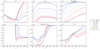	Fig. 8. Same as in Fig. 7, but for different values of the magnetic parameter αB.
In the text

Fig. 9. Properties of the corona on the radius (R/Rschw) – accretion rate (ṁ) parameter plane. All models are calculated for MBH = 10M⊙, αB = 0.1, and ξ = 0.05. The panels display (a) the average temperature of the corona (Eq. (44)) in keV (colors) and τcor (contours); (b) the ionization parameter Ξ (colors) and magnetic β parameter (contours), both at the disk midplane; (c) the number density at τ = 2/3 (colors) and the total column density Σ in g cm2 (contours); (d) the fraction of radiative energy produced by the corona f (Eq. (45), colors), the maximum value of the magnetic field gradient q (Eq. (35), contours); (e) the y parameter of the warm corona (Eq. (46)), computed up to the thermalization layer τ⋆ = 1 (colors) and to τcor (contours); the (f) photon destruction probability $ϵ={\kappa }_{\mathrm{ff}}^{\mathrm{P}}/{\kappa }^{\mathrm{P}}$ (colors) and electron scattering optical depth (τes) (contours) at the thermalization layer; (g) the minimum value of ℒrad (Eq. (37)) throughout the disk height (colors), here, green areas are stable disks, and magenta areas indicate thermal instability in the corona, the gray dotted line corresponds to ℒrad = 0, and the ionization parameter Ξ at the corona base (contours); and (h) the radiative energy flux normalized to the total accretion flux (colors), and the disk scale ratio H/R (contours).

In the text

	Fig. 10. Same as in Fig. 9, but on the radius (R/Rschw) – toroidal field production parameter (αB) plane.
In the text

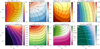	Fig. 11. Same as Fig. 9, but on toroidal field production parameter (αB) – accretion rate (ṁ) plane.
In the text

Fig. 12. Radial profiles of selected quantities: gas density ρ [cm−3], average temperature Tavg [K], and average Compton yavg (Eq. (46)), measured at different depths in the disk atmosphere. Values at τ = 0.1, τ = 1, and τ = 10 are shown by dashed blue lines, at temperature minimum (τcor) by the green line, at thermalization depth by the red line, and at the corona base (determined by temperature minimum or thermal instability in case it is developed) with the black dotted line.

In the text

References

- Anderson, E., Bai, Z., Dongarra, J., et al. 1990, in Proceedings of the 1990 ACM/IEEE Conference on Supercomputing, Supercomputing ’90 (Los Alamitos, CA, USA: IEEE Computer Society Press), 2 [Google Scholar]
- Bai, X.-N., & Stone, J. M. 2013, ApJ, 767, 30 [NASA ADS] [CrossRef] [Google Scholar]
- Balbus, S. A., & Hawley, J. F. 1991, ApJ, 376, 214 [NASA ADS] [CrossRef] [Google Scholar]
- Ballantyne, D. R., Ross, R. R., & Fabian, A. C. 2001, MNRAS, 327, 10 [NASA ADS] [CrossRef] [Google Scholar]
- Beckwith, K., Hawley, J. F., & Krolik, J. H. 2009, ApJ, 707, 428 [NASA ADS] [CrossRef] [Google Scholar]
- Begelman, M. C., & Pringle, J. E. 2007, MNRAS, 375, 1070 [NASA ADS] [CrossRef] [Google Scholar]
- Begelman, M. C., Armitage, P. J., & Reynolds, C. S. 2015, ApJ, 809, 118 [NASA ADS] [CrossRef] [Google Scholar]
- Di Salvo, T., Done, C., Życki, P. T., Burderi, L., & Robba, N. R. 2001, ApJ, 547, 1024 [NASA ADS] [CrossRef] [Google Scholar]
- Done, C., Davis, S. W., Jin, C., Blaes, O., & Ward, M. 2012, MNRAS, 420, 1848 [NASA ADS] [CrossRef] [Google Scholar]
- García, J. A., Kara, E., Walton, D., et al. 2019, ApJ, 871, 88 [NASA ADS] [CrossRef] [Google Scholar]
- Gierliński, M., & Done, C. 2004, MNRAS, 349, L7 [NASA ADS] [CrossRef] [Google Scholar]
- Gierliński, M., Zdziarski, A. A., Poutanen, J., et al. 1999, MNRAS, 309, 496 [NASA ADS] [CrossRef] [Google Scholar]
- Gladstone, J. C., Roberts, T. P., & Done, C. 2009, MNRAS, 397, 1836 [NASA ADS] [CrossRef] [Google Scholar]
- Goad, M. R., Roberts, T. P., Reeves, J. N., & Uttley, P. 2006, MNRAS, 365, 191 [NASA ADS] [CrossRef] [Google Scholar]
- Haardt, F., & Maraschi, L. 1991, ApJ, 380, L51 [NASA ADS] [CrossRef] [Google Scholar]
- Hawley, J. F. 2001, ApJ, 554, 534 [NASA ADS] [CrossRef] [Google Scholar]
- Hawley, J. F., & Balbus, S. A. 1991, ApJ, 376, 223 [NASA ADS] [CrossRef] [Google Scholar]
- Henyey, L. G., Forbes, J. E., & Gould, N. L. 1964, ApJ, 139, 306 [NASA ADS] [CrossRef] [Google Scholar]
- Hirose, S., Krolik, J. H., & Stone, J. M. 2006, ApJ, 640, 901 [NASA ADS] [CrossRef] [Google Scholar]
- Hirose, S., Krolik, J. H., & Blaes, O. 2009, ApJ, 691, 16 [NASA ADS] [CrossRef] [Google Scholar]
- Jiang, Y.-F., Stone, J. M., & Davis, S. W. 2014, ApJ, 784, 169 [NASA ADS] [CrossRef] [Google Scholar]
- Jin, C., Ward, M., Done, C., & Gelbord, J. 2012, MNRAS, 420, 1825 [NASA ADS] [CrossRef] [Google Scholar]
- Keek, L., & Ballantyne, D. R. 2016, MNRAS, 456, 2722 [NASA ADS] [CrossRef] [Google Scholar]
- Krolik, J. H., & Kriss, G. A. 1995, ApJ, 447, 512 [NASA ADS] [CrossRef] [Google Scholar]
- Krolik, J. H., McKee, C. F., & Tarter, C. B. 1981, ApJ, 249, 422 [NASA ADS] [CrossRef] [Google Scholar]
- Kusunose, M., & Mineshige, S. 1994, ApJ, 423, 600 [NASA ADS] [CrossRef] [Google Scholar]
- Laor, A., Fiore, F., Elvis, M., Wilkes, B. J., & McDowell, J. C. 1994, ApJ, 435, 611 [NASA ADS] [CrossRef] [Google Scholar]
- Laor, A., Fiore, F., Elvis, M., Wilkes, B. J., & McDowell, J. C. 1997, ApJ, 477, 93 [NASA ADS] [CrossRef] [Google Scholar]
- Liska, M. T. P., Tchekhovskoy, A., & Quataert, E. 2018, ArXiv e-prints [arXiv:1809.04608] [Google Scholar]
- Madau, P. 1988, ApJ, 327, 116 [NASA ADS] [CrossRef] [Google Scholar]
- Madej, J., & Różańska, A. 2004, MNRAS, 347, 1266 [NASA ADS] [CrossRef] [Google Scholar]
- Magdziarz, P., Blaes, O. M., Zdziarski, A. A., Johnson, W. N., & Smith, D. A. 1998, MNRAS, 301, 179 [NASA ADS] [CrossRef] [Google Scholar]
- McKinney, J. C., Tchekhovskoy, A., & Blandford, R. D. 2012, MNRAS, 423, 3083 [NASA ADS] [CrossRef] [Google Scholar]
- Mehdipour, M., Branduardi-Raymont, G., Kaastra, J. S., et al. 2011, A&A, 534, A39 [NASA ADS] [CrossRef] [EDP Sciences] [Google Scholar]
- Meurer, A., Smith, C. P., Paprocki, M., et al. 2017, PeerJ Comput. Sci., 3, e103 [CrossRef] [Google Scholar]
- Miller, J. M., Raymond, J., Kallman, T. R., et al. 2014, ApJ, 788, 53 [NASA ADS] [CrossRef] [Google Scholar]
- Nakamura, K., & Osaki, Y. 1993, PASJ, 45, 775 [NASA ADS] [Google Scholar]
- Nayakshin, S., & Kallman, T. R. 2001, ApJ, 546, 406 [NASA ADS] [CrossRef] [Google Scholar]
- Nayakshin, S., Kazanas, D., & Kallman, T. R. 2000, ApJ, 537, 833 [NASA ADS] [CrossRef] [Google Scholar]
- Noble, S. C., Krolik, J. H., Schnittman, J. D., & Hawley, J. F. 2011, ApJ, 743, 115 [NASA ADS] [CrossRef] [Google Scholar]
- Ohsuga, K., & Mineshige, S. 2011, ApJ, 736, 2 [NASA ADS] [CrossRef] [Google Scholar]
- Penna, R. F., Kulkarni, A., & Narayan, R. 2013, A&A, 559, A116 [NASA ADS] [CrossRef] [EDP Sciences] [Google Scholar]
- Pessah, M. E., & Psaltis, D. 2005, ApJ, 628, 879 [NASA ADS] [CrossRef] [Google Scholar]
- Petrucci, P.-O., Paltani, S., Malzac, J., et al. 2013, A&A, 549, A73 [NASA ADS] [CrossRef] [EDP Sciences] [Google Scholar]
- Petrucci, P. O., Ursini, F., De Rosa, A., et al. 2018, A&A, 611, A59 [NASA ADS] [CrossRef] [EDP Sciences] [Google Scholar]
- Piconcelli, E., Jimenez-Bailón, E., Guainazzi, M., et al. 2005, A&A, 432, 15 [NASA ADS] [CrossRef] [EDP Sciences] [Google Scholar]
- Pounds, K. A., Stanger, V. J., Turner, T. J., King, A. R., & Czerny, B. 1987, MNRAS, 224, 443 [NASA ADS] [CrossRef] [Google Scholar]
- Proga, D., & Waters, T. 2015, ApJ, 804, 137 [NASA ADS] [CrossRef] [Google Scholar]
- Różańska, A. 1999, MNRAS, 308, 751 [NASA ADS] [CrossRef] [Google Scholar]
- Różańska, A., & Czerny, B. 1996, Acta Astron., 46, 233 [NASA ADS] [Google Scholar]
- Różańska, A., Czerny, B., Życki, P. T., & Pojmański, G. 1999, MNRAS, 305, 481 [NASA ADS] [CrossRef] [Google Scholar]
- Różańska, A., Dumont, A.-M., Czerny, B., & Collin, S. 2002, MNRAS, 332, 799 [NASA ADS] [CrossRef] [Google Scholar]
- Różańska, A., Madej, J., Konorski, P., & Sądowski, A. 2011, A&A, 527, A47 [NASA ADS] [CrossRef] [EDP Sciences] [Google Scholar]
- Różańska, A., Malzac, J., Belmont, R., Czerny, B., & Petrucci, P.-O. 2015, A&A, 580, A77 [NASA ADS] [CrossRef] [EDP Sciences] [Google Scholar]
- Rybicki, G., & Lightman, A. 2008, Radiative Processes in Astrophysics, Physics Textbook (New York: Wiley) [Google Scholar]
- Salvesen, G., Simon, J. B., Armitage, P. J., & Begelman, M. C. 2016, MNRAS, 457, 857 [NASA ADS] [CrossRef] [Google Scholar]
- Sądowski, A., Wielgus, M., Narayan, R., et al. 2017, MNRAS, 466, 705 [NASA ADS] [CrossRef] [Google Scholar]
- Schnittman, J. D., & Krolik, J. H. 2010, ApJ, 712, 908 [NASA ADS] [CrossRef] [Google Scholar]
- Schnittman, J. D., Krolik, J. H., & Noble, S. C. 2016, ApJ, 819, 48 [NASA ADS] [CrossRef] [Google Scholar]
- Seifina, E., Titarchuk, L., & Shaposhnikov, N. 2016, ApJ, 821, 23 [NASA ADS] [CrossRef] [Google Scholar]
- Seifina, E., Chekhtman, A., & Titarchuk, L. 2018, A&A, 613, A48 [NASA ADS] [CrossRef] [EDP Sciences] [Google Scholar]
- Shakura, N. I., & Sunyaev, R. A. 1973, A&A, 24, 337 [NASA ADS] [Google Scholar]
- Shaposhnikov, N., & Titarchuk, L. 2006, ApJ, 643, 1098 [NASA ADS] [CrossRef] [Google Scholar]
- Stobbart, A.-M., Roberts, T. P., & Wilms, J. 2006, MNRAS, 368, 397 [NASA ADS] [CrossRef] [Google Scholar]
- Stone, J. M., Gardiner, T. A., Teuben, P., Hawley, J. F., & Simon, J. B. 2008, ApJS, 178, 137 [NASA ADS] [CrossRef] [Google Scholar]
- Svensson, R., & Zdziarski, A. A. 1994, ApJ, 436, 599 [NASA ADS] [CrossRef] [Google Scholar]
- Tange, O. 2011, The USENIX Magazine, 36, 42 [Google Scholar]
- Tout, C. A., & Pringle, J. E. 1992, MNRAS, 259, 604 [NASA ADS] [Google Scholar]
- Turner, N. J. 2004, ApJ, 605, L45 [NASA ADS] [CrossRef] [Google Scholar]
- Wu, M.-C., Xie, F.-G., Yuan, Y.-F., & Gan, Z. 2016, MNRAS, 459, 1543 [NASA ADS] [CrossRef] [Google Scholar]
- Yamada, S., Torii, S., Mineshige, S., et al. 2013, ApJ, 767, L35 [NASA ADS] [CrossRef] [Google Scholar]
- Yang, Q.-X., Xie, F.-G., Yuan, F., et al. 2015, MNRAS, 447, 1692 [NASA ADS] [CrossRef] [Google Scholar]
- Zhang, S. N., Cui, W., Chen, W., et al. 2000, Science, 287, 1239 [NASA ADS] [CrossRef] [Google Scholar]
- Życki, P. T., Done, C., & Smith, D. A. 2001, MNRAS, 326, 1367 [NASA ADS] [CrossRef] [Google Scholar]