| Issue |
A&A
Volume 672, April 2023
|
|
|---|---|---|
| Article Number | A19 | |
| Number of page(s) | 21 | |
| Section | Astrophysical processes | |
| DOI | https://doi.org/10.1051/0004-6361/202243828 | |
| Published online | 23 March 2023 | |
Modified models of radiation pressure instability applied to 10, 105, and 107 M⊙ accreting black holes
1
Nicolaus Copernicus Astronomical Center (PAN), ul. Bartycka 18, 00-716 Warsaw, Poland
e-mail: This email address is being protected from spambots. You need JavaScript enabled to view it.
2
Center for Theoretical Physics, Polish Academy of Sciences, Al. Lotników 32/46, 02-668 Warsaw, Poland
3
School of Physics and Astronomy, Tel Aviv University, Tel Aviv 69978, Israel
Received:
21
April
2022
Accepted:
21
January
2023
Abstract
Context. Some accreting black holes exhibit much stronger variability patterns than the usual stochastic variations. Radiation pressure instability is one of the proposed mechanisms that might account for this effect.
Aims. We model luminosity changes for objects with a black hole mass of 10, 105, and 107 solar masses, using the time-dependent evolution of an accretion disk that is unstable as a result of the dominant radiation pressure. We concentrate on the outburst timescales. We explore the influence of the hot coronal flow above the cold disk, the inner purely hot flow, and the effect of the magnetic field on the time evolution of the disk-corona system. For intermediate-mass black holes and active galactic nuclei, we also explore the role of the disk outer radius because a disk that is fed by tidal disruption events (TDE) can be quite small.
Methods. We used a 1D vertically integrated time-dependent numerical scheme that models the simultaneous evolution of the disk and corona, which is coupled by the vertical mass exchange. We parameterized the strength of the large-scale toroidal magnetic fields according to a local accretion rate. We also discuss a possible inner optically thin flow, the advection-dominated accretion flow (ADAF). This flow would require modification of the inner boundary condition of the cold disk flow. For the set of the global parameters, we calculated the variability timescales and outburst amplitudes of the disk and the corona.
Results. We found that the role of the inner ADAF and the accreting corona are relatively unimportant, but the outburst character strongly depends on the magnetic field and on the outer radius of the disk if this radius is smaller (due to the TDE phenomenon) than the size of the instability zone in a stationary disk with infinite radius. For microquasars, the dependence on the magnetic field is monotonic, and the period decreases with the field strength. For higher black hole masses, the dependence is nonmonotonic, and an initial rise of the period is later replaced with a relatively rapid decrease as the magnetic field continues to rise. A still stronger magnetic field stabilizes the disk. When we assumed a smaller disk outer radiusfor 105 and 107 M⊙, the outbursts were shorter and led to complex multiscale outbursts for some parameters, thus approaching the behavior of deterministic chaos.
Conclusions. Our computations confirm that the radiation pressure instability model can account for heartbeat states in microquasars. The rapid variability detected in intermediate-mass black holes in the form of quasi-periodic eruptions can be consistent with the model, but only when it is combined with the TDE phenomenon. The yearly repeating variability in changing-look active galactic nuclei in our model also requires a small outer radius either due to the recent TDE or due to the gap in the disk that is related to a secondary black hole.
Key words: accretion, accretion disks
© The Authors 2023
 Open Access article, published by EDP Sciences, under the terms of the Creative Commons Attribution License (https://creativecommons.org/licenses/by/4.0), which permits unrestricted use, distribution, and reproduction in any medium, provided the original work is properly cited.
This article is published in open access under the Subscribe to Open model. This email address is being protected from spambots. You need JavaScript enabled to view it. to support open access publication.
1. Introduction
The variability around black holes across their mass range shows different patterns of the amplitudes, shapes of the light curves, and timescales. The interpretation of the physical nature of these changes is difficult. Part of the variability is stochastic in nature, and these stochastic variations are seen both in X-rays and in the optical band (e.g., Lehto et al. 1993; Czerny et al. 1999; Gaskell & Klimek 2003; Krishnan et al. 2021). However, in some sources, the variations are much stronger than the usual stochastic changes. We do not consider the well-known state transitions in X-ray binary systems here, which occur on timescales of days and correspond to the viscous evolution of the outer disk. We study much more rapid and sometimes regular changes in the source luminosity.
For example, in the case of microquasars (whose black hole masses are in the range of 5–20 M⊙), the changes appear on timescales of tens to hundreds of seconds. Regular quasi-periodic outbursts with a period that depends on the mean flux were observed in GRS 1915+105 (Belloni et al. 2000). This regular variability was well modeled by the radiation pressure instability in the central parts of the accretion disk (Pringle et al. 1973; Lightman & Eardley 1974; Nayakshin et al. 2000; Janiuk et al. 2000, 2002). A similar so-called heartbeat variability of the microquasar IGR J17091 (RA: 01h19m08.68s Dec: −34d11m30.5s after NED1) was discovered by Altamirano et al. (2011), and its luminosity changes in X-ray band were also modeled by Janiuk et al. (2015) by the accretion disk radiation pressure instability. However, this source recently returned to the quiescent state (Pereyra et al. 2020). On the other hand, Bagnoli (2015) discovered heartbeat states in MXB 1730-335 (the Rapid Burster) that were later explored by Maselli et al. (2018).
Interesting semi-periodic variations were also discovered in the source HLX-1, which is located in the galaxy ESO 243-49. This source most likely contains an intermediate-mass black hole (IMBH) of 105 M⊙, and it underwent recurrent outbursts on a timescale of 400 days (Yan et al. 2015). The behavior of this source was also well modeled by the radiation pressure instability (Wu et al. 2016).
For more massive sources such as active galactic nuclei (in which the typical mass of the central black hole is about 107 M⊙), a phenomenon that exceeds stochastic variability is the occasional change in their spectral state. Major changes in Active Galactic Nuclei (AGN) structure an appearance were not expected because the characteristic timescales of accretion disks in AGNs are long because of their size. Nevertheless, large variations in the AGNs properties were occasionally reported in the past, both in X-rays and in the optical band, but systematic studies of these changes, including their classification, started much later. Historically, one of the first semi-periodic changes in the intensity of the Hβ line was reported for NGC 1566 by Alloin et al. (1986), but the name changing-look (CL) AGNs was introduced by Matt et al. (2003) and Bianchi et al. (2005) in the context of AGNs that changed from Compton-thin to Compton-thick or the reverse in their X-ray spectral shape. The two phenomena may be related, as indicated by a change both in the optical and in the X-ray spectrum in some sources (e.g., Masterson et al. 2022 in 1ES 1927, or Shappee et al. 2014 in NGC 2717) but in other sources, X-ray and optical changes are not always correlated, or not enough data coverage is available in both bands. Tidal disruption events (TDE) traditionally from a separate class, and they were searched for and found in otherwise inactive galaxies. When a TDE event occurs in an active or weak nucleus, however, it can also lead to a phenomenon similar to CL AGN. The typical observed timescales of these changes are rather counted in years (see introductions to recent papers, e.g., Yang et al. 2018; Noda & Done 2018; Trakhtenbrot et al. 2019; Graham et al. 2020; Oknyansky et al. 2019; Śniegowska et al. 2020). Changes in CL AGNs may thus be caused by more than one mechanism, which opens the possibility of modeling and exploring different scenarios for these phenomena.
Several mechanisms are presented in the literature. Ross et al. (2018) proposed instability at the boundary between the cold disk and the ADAF caused by magnetic fields threading the inner disk for source J1100-0053. Noda & Done (2018) discussed the temporary disappearance of the warm corona for Mrk 1018. For the same object, Feng et al. (2021) proposed magnetic accretion disk outflows. The authors modeled the UV/optical spectral shape of Mrk 1018 and consistently reproduced the observed changes. Supermassive black hole binaries, which may cause tidal interaction between disks that lead to state changes, were suggested by Wang & Bon (2020) as a possible scenario. Scepi et al. (2021) proposed that in source 1ES 1927+654, the CL event results from a reversing magnetic field. This was motivated by analogy with the 11-year solar cycle, and the field reversals and changes in accretion rate were indeed seen in MHD simulations of magnetically arrested disks. Raj & Nixon (2021) simulated the tearing disk structure, which may cause instabilities in the inner accretion flow (see also Raj et al. 2021, and references therein).
In the current paper, we concentrate on the special cases in which the CL phenomenon repeats in a given source. We do not focus on the actual character of the changes or on a specific energy band, but on the timescales of the process, combined with the repeating pattern. This quasi-periodic behavior rules out TDE or obscuration events, but opens the possibility of interpreting it as a limit-cycle operating in an unstable accretion disk. This is a challenging issue because the viscous timescales in AGNs disks are long, on the order of hundreds or thousands of years, if the entire radiation-dominated region participates in the evolution (e.g., Czerny 2006; Janiuk & Czerny 2011).
NGC 1566 is an example of a CL AGN with semiregular outbursts observed in the optical band (Alloin et al. 1986; Oknyansky et al. 2019). When we assume that thermal/viscous instability is led by radiation pressure, we can mimic the outburst cycle. Śniegowska et al. (2020) proposed a simple time-dependent toy model of an accretion disk under radiation pressure instability, in which the timescale of the outbursts was regulated by the thickness of the unstable zone. Pan et al. (2021) presented an extension of the Śniegowska et al. (2020) model by adding a magnetic field and showed that the timescale of the outbursts can be significantly reduced by the magnetic fields. The possibility of shortening the timescales in CL AGN phenomena by magnetization of the accretion disk was also suggested by Dexter & Begelman (2019).
Recently, a new, intriguing class of variable objects has been found. The first object was GSN 069 (Miniutti et al. 2019). This source is characterized by short and symmetric repetitive flares (every nine hours). Four more sources of similarly short eruption timescales have been found, and they are now known as quasi-periodic ejection events (RX J1301.9+2747, Giustini et al. 2020; eRO-QPE1 and eRO-QPE, Arcodia et al. 2021; and 2MASXJ0249, Chakraborty et al. 2021). It is not clear whether they are related to CL AGN. King (2020) suggested that this might be a nearly missed TDE event. Similarly, Xian et al. (2021) suggested that these outbursts may be driven by star-disk collisions, and Zhao et al. (2022) showed with stellar evolution code MESA that hydrogen-deficient stars are good candidates for this scenario. Suková et al. (2021) proposed periodic plasmoid ejection by an in-spiralling star. Ingram et al. (2021) proposed a scenario in which the binary supermassive black holes (SMBHs) is self-lensing, while Metzger et al. (2022) proposed the Quasi-periodic Eruption (QPE) mechanism based on an orbital coplanarity of stars, in which at least one star overflows its Roche lobe and accretes onto the SMBH. For these four sources, the lack of broad emission lines in the optical band is also characteristic, and this feature rules out the possibility of estimating black hole masses independently using broad-line diagnostics. As Wevers et al. (2022a) pointed out, the emission lines reported in these sources are typical of star-forming or accreting galaxies.
Our goal in this paper is to test the expected properties of accreting black hole sources under the radiation pressure instability. With this aim, we obtain a grid of models based on radiation pressure instability with considerable modifications to determine which of the observed timescales in different types of objects are consistent with the radiation pressure instability mechanism as the driving factor.
To perform this work, we used the time-dependent code Global Accretion Disk Instability Simulation (GLADIS)2, which was originally developed by Janiuk et al. (2002) and is now publicly available (Janiuk 2020). We modeled the accretion disk evolution by solving the equatorial disk temperature and the surface density time-dependent equations under the assumption of vertical hydrostatic equilibrium. We performed preliminary simulations for 107 M⊙ using the model in Śniegowska et al. (2022). However, the obtained outburst timescale was too long (more than 100 yr) in comparison to observed CL AGN. Thus, we decided to explore possible additional mechanisms that might shorten the period to a timescale of a few years.
In this work, we extend the model in GLADIS by adding a new boundary condition in order to represent the inner ADAF correctly. This is done by assuming a constant inflow of mass from the corona to the inner ADAF at the transition radius. We also account for an additional cooling component based on the idea of a dead zone (Begelman & Pringle 2007; Begelman et al. 2015) to shrink the outburst timescale without the damping effect. Finally, we study the potential role of TDE by allowing the disk outer radius to be much smaller than the full unstable zone in an infinite accretion disk (for these ranges, see Janiuk & Czerny 2011). We explore the properties of the model for 10 M⊙, 105 M⊙, and 107 M⊙ black hole masses, which correspond to a microquasar, the intermediate-mass source GSN 069 with QPEs, and the galaxy NGC 1566 with cyclic outbursts.
2. Model
We calculated the time evolution of the disk in a two-zone approximation of the vertical structure of the disk/coronal flow using the code GLADIS (Janiuk 2020). The disk structure and the corona structure at each radius were separately averaged vertically, as in the classical description of the disk (Shakura & Sunyaev 1973) or ADAF flow (Ichimaru 1977; Narayan & Yi 1994), but there was mass exchange between the two, parameterized as in Eq. (10), CASE (b) of Janiuk & Czerny (2007). We thus included the disk evaporation to the corona in a way dependent on the thermal state of the disk. We considered two options for the viscous dissipation and angular momentum transfer: a viscous torque proportional to the total pressure, αPtot, and a viscous torque parameterized by the geometrical mean between the total pressure and the gas pressure,  (Janiuk & Czerny 2011). We therefore do not discuss an even more general parameterization by the μ coefficient here, as in Szuszkiewicz (1990) and Grzędzielski et al. (2017). However, in comparison with previous code applications (Janiuk et al. 2000, 2002, 2015; Janiuk & Czerny 2011; Grzędzielski et al. 2017), we allow for three main modifications: the development of the inner ADAF zone, the modification of the vertical disk structure by the magnetic field, and the decrease in the disk outer radius.
The formation of the inner ADAF means that the cold disk disappears, and proper boundary conditions must be formulated to match the ADAF and the coronal flow in the outer disk. We illustrate the geometry of the model schematically in Fig. 1. Setting the outer disk radius at the arbitrary value in the case of AGN is motivated by the fact that the CL behavior might be related to TDE, and in this case, it may not be justified to assume a large enough outer radius of the disk to cover the whole instability zone, as was done in the papers cited above.
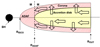 |
Fig. 1. Schematic view of the innermost part of the flow: Accretion disk (yellow), and hot corona above the disk (red), which transforms into an ADAF. The horizontal black line represents the equatorial plane. The vertical dashed line represents the boundary condition between the ADAF and outer flow. We perform computations between RADAF and Rout. |
2.1. Boundary condition between the ADAF and outer flow
We assumed that the transition radius between the inner ADAF and the outer two-zone disk/corona flow is set by the disappearance of the disk. The flow in the inner ADAF is stable, no mass accumulation is expected there. Therefore, because the disk no longer transfers mass at the transition radius, the continuity equation should be satisfied between the inner ADAF and the corona. The proper inner condition implies the constraints for the three innermost points of the radial grid because the equations are of second order. Point 0 is the innermost grid point where only the ADAF is present, which transfers all the material from the corona. We assumed
 (1)
(1)
for the coronal flow. Because  (see Eq. (27) in Janiuk et al. 2002), where Σcor is the surface density of the corona and
  is the radial velocity, we obtain by applying this equation to the condition above
 (2)
(2)
Here r0 = RADAF (see Fig. 1) in the presence of ADAF, otherwise r0 = 3RSchw.
The radial velocity in the corona was calculated as in Janiuk & Czerny (2007),
 (3)
(3)
where νcor is the kinematic viscosity of the corona.
When we consider three points r0, r1, and r2 and approximate the derivatives as the differences between two points Δr01 for the section r1 − r0 and Δr12 for the section r2 − r1 in the grid, we obtain the following expression for the velocity:
 (4)
(4)
for the left part of Eq. (2) and
 (5)
(5)
for the right part. Using these velocity expressions, we obtain
 (6)
(6)
and after simplification, we find the requested inner boundary condition for Σ0 as
![Mathematical equation: $$ \begin{aligned} \Sigma _0^\mathrm{cor} = \frac{r_1^{1/2}}{\nu _0} \left[\frac{\nu _1\Sigma _1^\mathrm{cor}}{r_0^{1/2}} + \frac{\Delta r_{01}}{r_0 \Delta r_{12}} \left( r_1^{1/2}\nu _1\Sigma _1^\mathrm{cor} - r_2^{1/2}\nu _2\Sigma _2^\mathrm{cor}\right) \right]. \end{aligned} $$](/articles/aa/full_html/2023/04/aa43828-22/aa43828-22-eq10.gif) (7)
(7)
The values of  and
and  were calculated from the time evolution equations. The inner ADAF thus transfers all the material that arrives through the corona in the innermost zone. This value of the surface density is time dependent and is derived from the quantities known in each new time step from time-dependent evolutionary equations. This boundary condition was only used when the inner radius is different than 3Rschw.
The condition above ensures that at the last disk radius, all material reaches the corona and later continues as a hot flow through ADAF toward the black hole. The accretion rate there is time dependent, forced by the evolution of the disk at all radii above RADAF. In the description of the dissipation, we used there zero-torque boundary condition, independently of whether RADAF > 3Rschw or the inner radius was set at ISCO. This is a simplification, and in general, another free parameter should describe the torque there (see, e.g., the approach by Zdziarski et al. 2022). This probably does not affect the evolution timescales.
2.2. Role of the magnetic field and appearance of the dead zone
In the standard accretion disk theory (Shakura & Sunyaev 1973), the magnetic field appears as a provider of the viscosity mechanism, parameterized through α. The actual mechanism behind this is the magnetorotational instability (MRI; Balbus & Hawley 1991). Its action has been seen in numerous MHD simulations (e.g., Fromang et al. 2007; Jiang et al. 2014; Pjanka & Stone 2020) as well as in experimental studies in the laboratory (see, e.g., Winarto et al. 2020, and references therein). However, as discussed by Begelman et al. (2015), MRI can lead to the generation of a toroidal magnetic field of considerable strength, and a dead zone can appear in the middle of the vertical disk structure, where MRI ceases to operate but magnetic energy continues to flow upward. This considerably modifies the effective vertical structure.
The criterion for the development of a dead zone from Begelman & Pringle (2007, Eq. (7) therein; see also the discussion in Begelman et al. 2015) is
 (8)
(8)
where vA represents the Alfvén speed, cs represents the speed of sound, and  and
and  . The scaling of the magnetic field pressure with the gas plus radiation pressure requires an additional parameter β,
 (9)
(9)
The criterion for dead zone formation therefore is
 (10)
(10)
We can evaluate when this criterion is satisfied using the hydrostatic equilibrium,
 (11)
(11)
With the use of Eq. (11), the condition for the formation of a dead zone reduces to
 (12)
(12)
We have two most extreme possible cases: gas-pressure dominance, and radiation-pressure dominance.
(i) Dominance of Pgas, Ptot = Pgas
In this case, the disk is geometrically thin, H/r is much smaller than 1, and the criterion is never satisfied for a geometrically thin disk.
(ii) Dominance of Prad, Ptot = Prad.
In this case, no simple analytical conclusion can be obtained. For the radiation-dominated disk branch, the vertical structure may – and likely will – therefore be modified, as argued by Begelman et al. (2015), and the strength of this modification depends on specific parameters.
The criterion of Begelman & Pringle (2007) applies to a strongly ionized plasma in which the turning off the MRI is related to the too strong magnetic field. At low accretion rates and/or large outer radii, another mechanism can in principle work. This mechanism is driven by the gas becoming too neutral and loosing the coupling to the magnetic field (see, e.g., Janiuk et al. 2004, and references therein). As shown by Janiuk et al. (2004), however, the MRI does not seem switch off in typical AGN through this mechanism.
Begelman et al. (2015) derived a formula that parameterizes the strength of the effect as the ratio of the standard disk height plus the dead zone to the standard disk height (see their Eq. (23)). The formula has a strong and interesting dependence on the dimensionless accretion rate with the power 29/99. We therefore applied it to modify the disk structure.
2.3. Modification of the cold disk structure by the magnetic field and stationary disk equations
In our model, we use a two-layer disk/corona approach as in Janiuk & Czerny (2007) instead of a full vertical structure. The corona is not affected, but we incorporate the possible effective modification of the disk zone due to the action of the magnetic field. Equation (23) in Begelman et al. (2015) implies the rise of the role of the magnetic field with dimensionless accretion rate. Because the application of the correction term to a vertically averaged disk structure is not unique, we introduce two specific prescriptions.
2.3.1. Model A
In this approach, we follow the general idea presented in Czerny et al. (2003), where we introduce energy transfer by the magnetic field in the form of Alfvén waves (upper panel of Fig. 2). This energy flux was thus proportional to the magnetic field B2, the Alfvén speed, vA, and the surface coverage by active regions. For this last effect, we lacked a convincing parameterization (we used the disk thickness). Now we propose to use the scaling with accretion rate from Begelman et al. (2015). The new energy flux thus becomes
 (13)
(13)
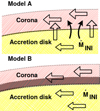 |
Fig. 2. Zoomed-in schematic view of the accretion flow from Fig. 1 with the modified structures that were introduced in the disk. Model A (upper panel) shows the energy transfer by the magnetic field in the form of Alfvén waves, represented as solid curved black arrows. Model B (bottom panel) shows the dead zone in the gray area between the corona and the accretion disk. |
where the magnetic field is assumed to scale with Ptot, and b is the arbitrary scaling constant. This magnetic energy transport is added to the general disk energy balance. This scaling implies that the role of the magnetic field is small at low accretion rates (when Pgas dominates), and rises for higher accretion rates. Thus, this formula is a smooth function with the expected properties, but without any onset threshold.
2.3.2. Model B
Following the idea of the dead zone of Begelman et al. (2015), we can expect that the role of the magnetic field scales with the relative width of the dead zone (bottom panel of Fig. 2). Since the scaling in Eq. (23) of Begelman et al. (2015) gives the ratio of z2/z1, where z2 is the zone plus the disk thickness, while z1 is the disk thickness, the global effect should scale as (z2 − z1)/z2. We cannot use the Compton coefficient here as in our time-dependent simulations of the mean zone this factor does not play a role. We therefore again used the scaling from Eq. (13) and arrived at the following modification term in our energy balance:
 (14)
(14)
where Ftot is the total locally dissipated flux. This requires the condition that the term PvA(ṁ)29/99 is larger than 1, otherwise, the term would be nominally negative. We then set it to zero. Here b′ is again an arbitrary proportionality constant.
We combined this new energy flux term (in the form of Eqs. (13) or (14)) with the usual equations of the stationary disk structure as follows. We used the vertically averaged relations for the total energy flux dissipating in the accretion disk (Eq. (19) in Janiuk et al. 2002),
 (15)
(15)
which in this case is generated through the α viscosity, where
 (16)
(16)
the local emitted flux
 (17)
(17)
 (18)
(18)
and the advection component
 (19)
(19)
Here the values Te, ρe, and Pe are the equatorial values of the temperature, density, and pressure, correspondingly, and H is the disk thickness. The coefficients C1 and C2 were calculated from the vertical disk structure at a fixed radius and were then used as universal parameters (see Janiuk et al. 2002). Combining these equations, we could write the energy balance equation for a given radius
 (20)
(20)
as was presented in Janiuk et al. (2002). For simplicity of the notation, we have dropped the indices e here, which indicate equatorial plane values.
Finally, by adding the additional magnetic transport cooling component to the energy balance equation (Eq. (20)), we obtain
 (21)
(21)
with the prescription for Fmag following Eqs. (13) or (14). Here we assumed αPtot viscosity, but we also considered the assumption  (see Szuszkiewicz 1990; Janiuk & Czerny 2011; Grzędzielski et al. 2017), which requires replacement of the corresponding dissipation term in the equations above. In the list of models, we refer to the first option as iPtot and to the second option as isqrt. These equations allow us to obtain the local stability curves for stationary models at each radius, set by the value of the black hole mass, viscosity parameter α, and the magnetic field parameter b or b′.
2.4. Time evolution of the disk/corona system
In addition to the modifications described in Sects. 2.1 and 2.3, we followed the time evolution of the disk/corona system as described in Janiuk & Czerny (2007). Both the disk and the corona evolve, and the disk mass is evaporated slowly to the corona, according to Eq. (10) of Janiuk & Czerny (2007). The local effect of the magnetic field related to MRI was included assuming that its time-dependence can be well represented by the Markoff process. The stochastic variations in the magnetic field affect the coronal outflow, and, indirectly, the underlying disk. This model thus includes the stochastic variability of the flow, which may be coupled with large-scale radiation pressure instability, leading to periodic outbursts. Because we now introduce additional modifications to the model of Janiuk & Czerny (2007), we list the full set of time-dependent equations below.
For the accretion disk evolution, we solved two equations: The equation of mass and angular momentum conservation,
 (22)
(22)
and the energy equation,
 (23)
(23)
In the case of the equation of mass and angular momentum conservation, we used the following term (one of three possible mechanisms; see Janiuk & Czerny 2007, and their Eq. (10) (case B) for the disk evaporation ṁz into corona:  ). The magnetic field in this model evolves in a complex way: fast intrinsic variation is modeled as a stochastic variability related to the local MRI and evolved as a discreet Markoff process as suggested by King et al. (2004) and Mayer & Pringle (2006), and part of the evolution is coupled to the change of the interior disk parameters because the maximum of the magnetic field is set by the value of the total pressure at the equator, that is,
 (24)
(24)
Here the Markoff chain value un has a mean value of zero, a dispersion of 1, a memory coefficient of α1 = −0.5, and the local time step is proportional to the local dynamical timescale (see Janiuk & Czerny 2007). When the energy equation β is  and vr is the radial velocity in the disk, Q+ is viscous heating, Q− is radiative cooling, and Fmag is an additional cooling component (from model A or model B), with dimensionless factor, b, whose possible values we investigate in this work. For the evolution of corona, we solved only the mass and angular momentum conservation because we assumed the virial temperature such that the temperature at each radius was fixed,
 (25)
(25)
3. Results
Before we show the results for the time evolution of the disk under the radiation pressure instability, we briefly present a few characteristic properties of the current model, modified concerning the one used by Janiuk & Czerny (2007). This helps later to understand some of the new evolutionary trends. Since stationary models are purely local (interaction with nearby radii are set by the stationarity condition), they can only display well the role of the magnetic field through modification of the disk’s vertical structure.
3.1. Stationary solutions and exemplary stability curves
As we show in Sect. 2.3, the energy balance is affected by the modification of the energy flux that mimics a magnetic field (Eq. (21)). We show the S-curve of the local surface density versus temperature plane for model A for various coefficients in Fig. 3 and for model B for various coefficients in Fig. 4. These curves represent the local disk structure under the condition of thermal balance. These are stationary models, therefore various values of the disk temperature correspond to various values of the accretion rate. We plot them for three different black hole masses: 10 M⊙, 105 M⊙, and 107 M⊙. In all cases, we performed the computations at the radius of 10RSchw, and we assumed the viscosity parameter α = 0.01.
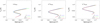 |
Fig. 3. Local stability curves for black hole masses for 10 M⊙ (left panel), 105 M⊙ (middle panel), and 107 M⊙ (right panel). For each curve, we keep R = 10Rschw and α = 0.01. The color of the S-curve represents different coefficient values for model A: blue for b = 0 (base model), green for b = 0.1, and red for b = 0.15. For each plot, we keep the same X-axis and the same range (3 orders of magnitude) for the Y-axis. |
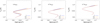 |
Fig. 4. Local stability curves for black hole masses for 10 M⊙ (left panel), 105 M⊙ (middle panel), and 107 M⊙ (right panel). For each curve, we keep R = 10Rschw and α = 0.01. The color of the S-curve represents different coefficient values for model B: blue for b′ = 0 (base model), orange for b′ = 0.5, and brown for b′ = 0.9. For each plot, we keep the same X-axis and the same range (3 orders of magnitude) for the Y-axis. |
The shape of the S-curve provides direct information about the local stability of the disk because positive branches correspond to stable solutions and negative slopes correspond to unstable ones. The disk evolution estimated locally would manifest as a loop in these plots, with the stages of slow evolution along the stable branches and rapid vertical transitions on thermal timescales between the stable branches. The extension of the unstable branch allows for an estimate of the amplitude and the duration of the full cycle, but only locally. The global evolution is the combined effect of the processes at all radii. Nevertheless, the change in the S-curve shape when the magnetic field effects are introduced shows the likely trend in the global evolution.
In the case of model A, S-curves are shifted horizontally (apart from lower stable branch) and the lower turning point seems to slightly shift vertically. The effect vanishes with increasing black hole mass. The separation between the minimum and maximum value of the temperature at the unstable branch becomes somewhat lower with the rising value of the parameter b, therefore we rather expect a lower outburst amplitude. The minimum value of the density at the unstable branch becomes higher, so that after the collapse of the disk onto the lower branch, its local accretion rate is higher and the viscous timescales are shorter with the rise of b. The effect of the magnetic field, however, seems to be relatively weaker for higher masses.
In the case of model B, the flattening of the unstable part of the curve is again observed, implying expectations of a lower outburst amplitude. However, the upper point of the unstable branch seems to be unaffected by the change in the parameter b′, therefore the outburst timescale may not be reduced in this case. Again, the changes in the S-curve shape at higher accretion rates are smaller. A similar effect (in the shape) of the upper branch of the stability curves was obtained by introducing vertical outflows (Janiuk et al. 2002, see Fig. 3 therein).
Summarizing, the curves are modified by the effect of the magnetic field in the disk interior, but the modifications in both models (A and B) do not seem to be very strong, especially in the case of higher black hole masses. However, the local study of the S-curve can only indicate trends, while actual properties of the disk time evolution can be only assessed by performing a global evolution of the disk. The effects of the inner and outer boundary conditions are seen only in the global simulations.
3.2. Time-dependent evolution
Our global model of the accretion disk evolution has the following input parameters: black hole mass, MBH, accretion rate ṁ in Eddington units, the inner radius RADAF (or no ADAF, and then the inner radius is located at ISCO), the outer radius Rout, the type of the viscosity law (the viscosity parameter α was always fixed at the same value, 0.01), the type of the magnetic field modification and the coefficient (b or b′) scaling the strength of this effect, and the presence or absence of the hot accreting corona above the disk. We calculated several such global models, and their input parameters are listed in Tables A.1–A.3.
For each of the models, we calculated the standard output parameters: the period (if outbursts are present), which is measured from one peak to the next, the relative amplitude of the disk outburst (maximum to minimum flux), and the relative outburst amplitude of the corona. These results are given in the corresponding tables. Outburst amplitudes in the disk correspond to the total time-dependent luminosity of the disk, Ftot, coming from the local radiative flux integrated over the disk surface for each moment of the time evolution. The coronal luminosity was calculated in a time-dependent manner, first locally as the dissipation rate in accreting coronal flow, assuming α viscosity as in the disk, and then by integrating the coronal flux over the disk surface. We illustrate the results with exemplary light curves. From the point of view of the evolutionary timescales, the black hole mass is the key parameter because it determines the scale size of the object. We therefore first concentrated on the results for the MBH = 10 M⊙ and later proceed toward higher masses.
Before plotting the full light curves, we first illustrate an important difference between the stability curves discussed in Sect. 3.1 and the full time-dependent computations. To do this, we selected a model with MBH = 10 M⊙, accretion rate ṁ = 0.67, without a hot corona, or inner ADAF, and with the outer radius Rout = 300RSchw, which is large enough to cover the whole instability region, and without any additional effects of the magnetic field. We selected the representative radius of 40RSchw, and we plot in the left panel of Fig. 5 the evolution of the effective temperature and the surface density at this radius. In the right panel, we plot the small fragment of the total disk light curve. We indicate the characteristic parts of the light curve with different colors for a slow luminosity rise in the viscous timescale in red, a fast thermal rise, and a relatively fast viscous evolution along the hot branch in black, and then the decay in green. The same colors are used in the left panel, and arrows show the direction of the limit cycle. As a reference, we plot the stationary stability S-curve for their model at this radius, but the actual evolution clearly does not follow the stationary curve perfectly because the disk also evolved at smaller and larger radii, and the radial derivatives that affect the local disk state are also time dependent.
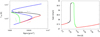 |
Fig. 5. Illustration of the limit cycle instability in the accretion disk. Left panel: local stability curve (blue line). The outburst cycle for a black hole mass 10 M⊙ and R = 40Rschw for a base model without RADAF and Rout = 300Rschw is indiated. Right panel: exemplary fragment of the disk light curve. The cycle steps are indicated for a black hole mass 10 M⊙. The following steps of the cycle are colored: the black part of the light curve represents the heating phase, the green part shows the advective phase, and the red part represents the diffusive phase. The colored arrows indicate the direction of the cycle anticlockwise. |
3.2.1. Microquasars
In this subsection, we fix the black hole mass value at 10 M⊙ so that we can concentrate on solutions that might be applicable to microquasars showing heartbeat states. We calculated a large set of models without the inner ADAF (i.e., RADAF = 3RSchw), in which the large outer radius did not affect the disk evolution (Rout = 300RSchw, the disk is already stable there), but without or with the corona, and with an increasing magnetic field parameter. For each of these models, we used the viscous torque proportional to the total (i.e., gas + radiation) pressure. A test model, with the square-root law for the viscous torque, was stable. Table A.1 shows that the presence of the corona does not affect the amplitude and the timescales of the outbursts strongly, therefore we plot the solutions with a corona because they contain additional information on the expected behavior of the hard X-rays.
We first analyze model A of the magnetic field effect. In Fig. 6 we plot the light curves for the disk and for the corona using the same timescale on the horizontal axis. This sequence of models shows that the outburst period is strongly reduced with the rise of parameter b (see Eq. (13)). Without the role of the magnetic field b = 0, the outburst period is about 0.1 day (2.4 h), while at the value b = 0.15, the period is reduced to 2 min. Higher values of parameter b give stable solutions. The reduction of the period is also accompanied by the reduction of the outburst amplitude. This again illustrates the fact that the stationary stability curves are shown in Figs. 3 and 4 do not predict the outbursts well, and computations of actual time-dependent global solutions are necessary. The outburst amplitudes in the corona are much smaller than the disk amplitudes in our model, and at b > 0.1, the corona is almost stable, except for the usual stochastic variability. In observations, the outbursts amplitudes are measured using count rates in the selected energy band, while in our theoretical model, we calculate bolometric luminosities, therefore the direct comparison with the data is not simple, but the radiation pressure instability model well represents the observed time delays between the hard X-ray and soft X-ray flux (Janiuk & Czerny 2005). We did not calculate the time delay because we concentrated on amplitudes and timescales.
 |
Fig. 6. Disk (gray) and corona (red) light curves for 10 M⊙ for different coefficient values b′ for model A (from the top left): b = 0 (base model), 0.09, and 0.15. For all cases, the inner radius is 3Rschw and the outer radius is Rout = 300Rschw. |
Next, we used the same basic setup, but assumed model B of the magnetic field effect on the disk structure (see Eq. (14)). We again calculated a sequence of models with increasing values of the parameter b′. We plot the models with the corona (see Fig. 7). The initial trend with the rise of the magnetic field is very similar to that of the A model family: the outbursts become shorter with the rise of the magnetic field term, the amplitudes become smaller, and the coronal outbursts have a smaller amplitude than the disk outbursts. For b′> 0.7, the outburst in the corona disappears and is again replaced with purely stochastic variations. However, there is an important difference with model A for the highest values of parameter b′. When b′ is changed from 0.97 to 1.0, the amplitude decreases, but the outburst duration increases from 16 min to 40 min, and the outburst shape changes: an extended plateau develops before the consecutive outbursts. The models without a corona follow the same pattern for low values of b′ (see the outburst timescales and amplitudes in Table A.1). However, the last model (b′ = 1.0) without a corona follows the trend of a shorter outburst scale (the outburst duration is 6 min), and no changes in the outburst shape are observed. A further increase in the parameter b′ leads to stable solutions. Therefore, the role of the magnetic field is critical from the points of view of disk stability, outburst amplitudes, and timescales. Two proposed descriptions (models A and B) imply a similar behavior, although with some differences in detail, as discussed.
 |
Fig. 7. Disk (gray) and corona (red) light curves for 10 M⊙ for different coefficient values b′ for model B (from the top left): b′ = 00.2, 0.5, 0.9, and 1.0. For all cases, the inner radius is 3RSchw and the outer radius Rout = 300Rschw. |
Next, we studied the dependence of the model on the inner ADAF hot flow. We used models of the disk with a corona because in this case, the boundary condition requires that the coronal material flows as ADAF below RADAF, and models without a corona cannot satisfy the boundary conditions as formulated in Sect. 2.1. We did not include the magnetic field effect. The expectation was that perhaps the coronal flow and fast inner ADAF flow may combine toward shortening the outbursts. However, computations show that the outburst period slightly increases. The amplitude decreases as the unstable region shrinks, and for an ADAF radius larger than 30, RSchw, the instability ceases to exist. The trend is illustrated in Fig. 8. Therefore, the inner ADAF can only damp the instability, but does not affect the outburst timescale considerably.
 |
Fig. 8. Disk (gray) and corona (red) light curve for 10 M⊙ with a modified boundary condition (for details, see Sect. 2.1) for different inner radii (RADAF) 3 (base model), 10, and 20Rschw. The outer radius for all cases is Rout = 300Rschw. |
In all previous computations, we assumed a rather high accretion rate, 0.67, as is appropriate, for example, for GRS 1915+105. We therefore determined the modification for models with somewhat lower accretion rates. For ṁ = 0.5 and model B without a corona, we observe the same trend as for the higher accretion rate: as the parameter b′ rises, the outburst timescales shrink and the amplitudes decrease. The trend is slightly more shallow than for a higher accretion rate, which means that the unmodified model shows a shorter timescale at a lower accretion rate, but at b′ = 0.5, both timescales are comparable.
Because we used a Markoff process to model the fast underlying stochastic variability (see Janiuk & Czerny 2007, for details), we also tested the role of the adopted the memory coefficient (α1 = −0.5 as default) on the results. However, the effect is weak, the change of α1 does not affect the period and the amplitude of the outbursts, but it slightly affects the luminosity of the corona: for coefficients −0.4 and −0.3, the luminosity of corona is lower, whereas for −0.6 and −0.7, it is higher.
In the case of a microquasar, we do not study the role of the outer radius because in this case, the mass supply comes from the companion and the radius of the entire disk is large. In time-dependent computations, it is necessary to cover just the entire unstable zone, and no effects of the outer radius are expected.
3.2.2. Intermediate-mass black holes
In this section, we discuss the results for a black hole mass of 105 M⊙, which is representative of sources such as HLX-1 or GSN 069. The model parameters are given in Table A.2. We usually set the value of the outer radius at 300RSchw. We show the dependence of the disk and corona evolution on the importance of the magnetic field assuming model A in Fig. 9. The characteristic timescales are much longer. In our basic model, the outbursts are 35.7 yr, and without the corona, the duration of the limit cycle is only slightly shorter (27.6 yr). However, we again observe a strong trend of a shorter period with increasing role of the magnetic field, and for b = 0.17, the period is reduced to 4.7 yr. A further increase of b stabilizes the disk, and the disk without a corona still shows outbursts for b = 0.22, and then the period is even shorter (1.1 yr). The outburst shapes are different from those for a black hole mass 10 M⊙. The duration of the bright phase is much shorter than the overall duration of the limit cycle. The light curves also show a dip and short minimum before the next outburst. However, a very interesting pattern appears when the accretion corona is not included. For b = 0.07, outbursts of the disk without a corona are still similar to an outburst with a corona, but for b = 0.09 or higher, secondary oscillations develop immediately after the dominant peak (see Fig. 10). The interaction with the corona damps this effect. However, similar complex substructure effects quite frequently appear in the computations of higher masses, and we discuss this below. Overall, the substructure here does not affect the limit of the cycle duration.
 |
Fig. 9. Disk (gray) and corona (red) light curve for 105 M⊙ for different b factors for model A. The inner radius is 3Rschw, and the outer radius is Rout = 300Rschw for all cases presented in this plot. |
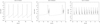 |
Fig. 10. Disk (gray) light curve for 105 M⊙ for different b factors for model A. The inner radius is RADAF = 3 and the outer radius is Rout = 300Rschw for all cases presented in this plot. The X-axes in plots are different. |
In both cases, with and without a corona, we observe an interesting trend for the limit in the cycle duration. For very low values of the parameter b, the duration slightly rises with increasing strength of the magnetic field, and only for b ∼ 0.07 does it start to decrease very fast. No such effect was seen in the microquasar case.
When we describe the magnetic field with model B, no substructure develops after the main peak. Single peaks occur, but with a similar profile as for model A: a very short bright phase, and a dip minimum after the peak (see Fig. 11). The limit of the cycle duration initially increases with the increase in the magnetic field effect and is later replaced with a decrease, down to timescales of 9 yr (without a corona) and 18 yr (with a corona). The corona affects the disk behavior quantitatively, but not qualitatively, in this case.
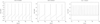 |
Fig. 11. Disk (gray) light curve for 105 M⊙ for different b′ factors for model B. The inner radius is 3Rschw, and the outer radius is Rout = 300Rschw for all cases presented in this plot. |
The effect of the inner ADAF for this mass scale did not affect the solutions considerably either. We calculated several models (see Table A.2), but as for the microquasar case, the timescale was weakly affected. Only the amplitude dropped with increasing RADAF, and the model became stable for RADAF above 30 RSchw. However, for the intermediate black hole mass scale, we decided to determine the role of the outer disk radius. The mass supply mechanism in the case of the intermediate black hole masses is not clear, and the mass source can determine the outer boundary conditions. Therefore, in addition to the standard value of Rout = 300RSchw, we calculated models with outer radii of 100RSchw and 50RSchw, without and with a corona. The change in outer radius has a clear and strong effect on the disk outbursts. Part of the potentially unstable disk is now simply removed (although mass is still supplied there), which removes the part that causes the longest local evolutionary timescales. The global effect goes as expected: the overall period of the outburst shortens significantly, from 27 yr to 0.9 yr for the smallest disk without a corona, and a corona does not change the trend. Because there is almost no difference in the disk behavior between the disk with and without a corona, we plot only the case with a corona in the top left panel of Fig. 12. In addition to the shortening of the outburst, the outburst character changes significantly.
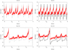 |
Fig. 12. Light curves with different numbers of grid points for 105 M⊙ and the inner radius is 3Rschw. Upper panel: light curves computed with different numbers of grid points (left panel: 98 points, and right panel: 34 points for the outer radius Rout = 50Rschw). Lower panel: 98 and 50 points for the outer radius Rout = 100Rschw. |
Outbursts of disk with an outer radius 300RSchw are almost identical. When the disks are smaller (i.e., 50RSchw), three outbursts with an incrasing amplitude occur instead. This behavior is expected, and it was seen, for example, in computations of the outbursts of cataclysmic variables caused by the ionization instability (see, e.g., Hameury et al. 1998, their Fig. 8). Because Hameury et al. (1998) argued that the exact shape of these complex outbursts depends on the computational grid, we also tested the grid assumption. In the top right panel of Fig. 12, we plot the results obtained with a smaller number of grid points whose position coincides with the grid used in models with Rout = 300RSchw. The exact sequence of subpeaks is modified (two-peak sequence instead of a three-peak sequence), but the complexity remains. We also plot the results for Rout = 100RSchw (Fig. 12, lower panel). In this last case, the effect of the change in grid resolution is small.
3.2.3. Supermassive black holes
Sections 3.2.1 and 3.2.2 showed that the magnetic field shortens the duration of the outburst in the radiation-pressure instability model. However, this effect is likely not strong enough when we aim to model CL AGN. The standard outburst timescales in AGNs are thousands of years (Czerny et al. 2009; Grzędzielski et al. 2017). On the other hand, as we already noted in the case of IMBH, the position of the outer radius can lead to much shorter outbursts. The small outer radius is predicted if the activity is actually caused by the TDE effect. In the current study, we therefore concentrate on the scenario in which the TDE is the underlying phenomenon, but the active evolutionary phase is long enough for the radiation pressure instability to act and a few cycles can be performed by the disk. We therefore assumed Rout = 100Rschw, and we studied the properties of this model, including modifications caused by the magnetic field. This radius is much smaller than the whole instability zone, which extends up to a few hundred RSchw (Janiuk & Czerny 2011), but in time-dependent computations, the regions above a thousand RSchw are still affected. Therefore, this is certainly the most important modification in comparison to the set of standard models discussed by Grzędzielski et al. (2017). All the models are listed in Table A.3. We assumed a lower accretion rate in these models, ṁ = 0.2, because CL AGNs are not too close to the Eddington rate.
The reference model shows an outburst period of 51 yr. The models of Grzędzielski et al. (2017) had a viscosity law parameter μ = 0.56, which is slightly higher than the outburst periods implied by the square-root law. These are on the order of 1000 yr. For the assumption of a torque proportional to the total pressure, as currently used, outbursts could not be calculated by Grzędzielski et al. (2017) because the outbursts were too longs, the instability rise was too steep, and because they encountered computational problems. The choice of much smaller outer radii in the current paper reduces the outburst timescales, amplitudes, and the steepness of the thermal rise of the luminosity so that no numerical problems are met.
We analyzed a further reduction of the outburst period in detail that might be caused by the action of the magnetic field. We used model B for this purpose. The results depended only weakly on the presence or absence of a corona. The trend was similar to what we already reported for the IMBH case: the period rose with the increasing strength of the magnetic field, parameterized by the coefficient b′. However, for higher masses, this rising trend continued to much higher values of b′ and reversed to shorten the limit cycle duration only for b′> 1.0. Then as before, for still higher values of b′, the period as well as the amplitude decrasesd, and for b′> 1.25, the disk became stable.
The model without a corona has similar properties as the model with an accreting corona. As for the IMBH case, the outbursts are very sharp, followed by a deep minimum. For example, the duration of the limit cycle for b′ = 1.0 (without a corona) lasts 235 yr, but the duration of the bright phase is about 20 yr. The influence of the change in grid resolution on the results is noticeable. Outbursts become shorter for a smaller number of grid points. This is clearly visible for the case of disk with the outer radius Rout = 50Rschw (see the upper panel of Fig. 12), in which the outburst periods decreased by a factor of 3. Furthermore, the outbursts are not identical, but alternate between stronger and weaker outbursts.
We determined the role of the inner ADAF in the case of massive black holes, but it again did not qualitatively affect the results, except for a systematic decrease in the outburst amplitude with rising RADAF. However, the role of the outer radius is dominant, so that we also tested the case of a still lower value, Rout = 50RSchw. In this case, we observe a similar phenomenon as for the IMBH: the time evolution became very complicated, with a sequence of outbursts of different heights that repeated regularly. The effect is only weakly affected by the presence or absence of a corona (see Fig. 13).
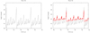 |
Fig. 13. Disk (gray) and corona (red) light curves for 107 M⊙ for an inner radius 3Rschw and an outer radius Rout = 50Rschw. |
3.2.4. Global trends across the mass scale and magnetic field strength
In the three previous subsections, we discussed the dependences of the outburst properties separately for each black hole mass. We showed that the period has a complex nonmonotonic dependence on the strength of the magnetic field for higher masses. To show the pattern more clearly, we plot the global output parameters, just the amplitude and the duration, for all three black hole masses next to each other, for model A in Fig. 14 and for model B in Fig. 15. Because the effect of the corona on the disk outburst parameters is weak, we only plot models without a corona in both cases.
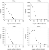 |
Fig. 14. Dependence on the amplitude of the outburst and period on magnetic coefficient for 10 M⊙ and 105 M⊙. Top panel: dependence on the amplitude of the outburst of the accretion disk and magnetic coefficient b for black hole masses of 10 M⊙ (left panel) 105 M⊙ (right panel). The bottom panel shows the dependence of the period on b for the same model parameters. All simulations in those plots were run for Rout = 300Rschw. The behavior of the period for higher masses is nonmonotonic. |
Figure 15 shows that the amplitude of the outburst decreases with field strength, independently of the black hole mass. However, in the case of the period, the trend in the pattern is clear. In the case of the IMBH, the period first rises and then decreases. In microquasars, we see only the second, decreasing branch, while for a supermassive black hole, the first, rising branch dominates, and the period becomes shorter for very high values of b′, and then the change is very rapid.
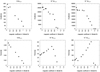 |
Fig. 15. Dependence on the amplitude of the outburst (top panel) and the duration of the limit cycle (lower panel) of the accretion disk and magnetic coefficient b′ for black hole masses of 10 M⊙ (left panel), 105 M⊙ (middle panel), and 107 M⊙ (right panel). |
These plots show that the amplitudes of the outbursts are rather large, and they rise with black hole mass. In the case of microquasars, the observed amplitudes in GRS 1915+105 are about 3–16 in the heartbeat states (Belloni et al. 2000). The observed timescales of these outbursts range from 40 s to 1500 s, and they weakly correlate with amplitude. Our set of models produces solutions like this when the effect of the magnetic field is strong. For example, b > 0.09 in model A without a corona gives the right period range, and b > 1.2 also gives the right amplitude. Model B predicts amplitudes that are slightly too high for the minimum period seen in the solutions. Another microquasar, IGR J17091-3624, has amplitudes up to a factor of 20, and the outburst timescales cover the range from 2 s to 100 s (Altamirano et al. 2011), which is shorter on average than in GRS 1915+105. This might be related to a somewhat lower value of the Eddington rate and the mass in this source. Our grid of models does not generally cover the mass and Eddington ratio grid densely, but the solution for ṁ = 0.5 shows a shorter period than the model with ṁ = 0.67 (0.06 vs. 0.09 day) for the same value of b′. It is also important to note that a relatively small further increase in the strength of the magnetic field stabilizes the disk, and this may be consistent with the fact that heartbeat states are not always present. We also decided to determine the importance of the black hole mass and ṁ assumed in our modeling. In the case of 10 M⊙, the period decreases a monotonically, whereas for 105 and 107 M⊙, it decreases and increases with b for model A. The models differ from each other in two parameters: mass, and accretion rate. To determine which of these is the leading parameter, we computed a few cases for 10 M⊙ with an accretion rate ṁ = 0.5 (the same as we used for 105 M⊙). For this simple test, we note a similar monotonic decrease in the period. Thus, we claim that the black hole mass is the leading parameter in this trend.
The comparison with the data is not precise because in the data, we measure the amplitude as the count rate, and this strongly depends on the selected energy band. In the models, however, we predict the bolometric luminosity of the disk. Moreover, when the corona luminosity is added to the disk, the amplitudes measured from the model can be smaller because the accreting corona has much lower outburst amplitudes than the disk.
When the model is applied to an IMBH, we can refer to observations of the outbursts in the object HLX-1, which shows regular outbursts with a timescale of 400 days, an amplitude of about a factor of 100 (Yan et al. 2015), and which was already successfully modeled as the effect of the radiation pressure instability (Wu et al. 2016; Grzędzielski et al. 2017). Solutions with these properties are characterized by a magnetic field strength of b ∼ 0.2 (model A). The timescales in model B are somewhat longer, and they rapidly become shorter for b′ between 1.0 and 1.1, when the model becomes stable. This leaves a very narrow range of potential parameters.
In Fig. 16 we present the dependence of the amplitude (left panel) and period (right panel) on the different outer radii without amagnetic field and without a corona for 105 M⊙. The amplitude strongly decreases with decreasing Rout. For Rout = 10RSchw, it is almost 70 times smaller than for Rout = 100RSchw. In the case of period versus Rout, the timescale decreases from 1.6 years for Rout = 100RSchw to ∼4 days for Rout = 10RSchw.
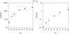 |
Fig. 16. Dependence on the amplitude of the outburst (left panel) and the duration of the limit cycle (right panel) for different short outer radii of the accretion disk for the black hole mass 105 M⊙. The effect of the magnetic field is not included. |
However, a new class of outbursts that is now known as QPEs has been detected. The black hole masses in these sources are in the range of IMBH masses or low-mass AGNs (4 × 10⁵ M⊙ in GSN 069; Miniutti et al. 2019, (0.8 − 2.8)×106 M⊙ in RX J1301.9+2747; Giustini et al. 2020, low but highly uncertain masses in eRO-QPE1 and eRO-QPE2; Arcodia et al. 2021). The timescale there is much shorter, on the order of some hours. Our results in Table A.2 for the outer radius of 300RSchw show the minimum of the limit cycle timescale of one year (model A, b = 0.22, no corona). The models with the smallest outer radius in our computations (50RSchw) implied a shortening of the outburst time by a factor of 30, which is more by a factor of 2 than the reduction of the timescale expected from the simplest scaling of the dynamical time with the radius (power 3/2). Therefore, recalculating the model mentioned above with b = 0.22 might shorten the outburst timescale to 10 days. We performed these calculations and present the result in Fig. 17. The period of the short small outbursts is about 8 days, but the object luminosity rises systematically, and small outbursts are accompanied by large outbursts. This shows that short timescales can be achieved in our model, and a further decrease in the outer radius can give still shorter timescales. The duration of the bright phase is shorter than the duration of the limit cycle, as observed in the QPE phenomena. However, we cannot yet claim full success in explaining QPE because the overall pattern may not be as expected. In the future, a much more careful approach to the outer boundary condition is needed.
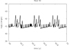 |
Fig. 17. Disk (black) light curve for 105 M⊙ for b′ = 0.22 factors for model A. The inner radius is 3Rschw, and the outer radius is Rout = 50Rschw. |
However, our results clearly show that short-timescale (hours) regular outbursts are consistent with the radiation pressure instability only in the case of very small outer disk radii. This means that the radiation pressure instability model can be applied to QPE events only under two conditions: (i) the general rise in the source activity must be due to the TDE effect, as this would limit the outer disk radius in a natural way, and (ii) the role of the magnetic field in the disk must be large. In the current paper, we did not aim to determine unique parameters for QPE sources because the black hole mass measurements in these sources are quite uncertain, but the conditions formulated above are generic. The QPE sources detected so far were indeed activated by TDE as they happened in previously inactive galaxies.
In higher black hole masses characteristic of typical AGN, we only considered TDE-powered events because we wished to determine whether rapid CL events can be explained by radiation pressure instability. The observed timescales in CL are poorly constrained because multiple events are rarely detected, and in the case of a single-transition event, the process is usually captured only poorly. However, the typical timescales range from months to years, which may also be a selection bias against longer-timescale changes that cannot be followed by optical instruments. Timescales as short as this again require a combination of a small outer radius (its reduction from 100 to 50RSchw reduces the period by a factor of 10) and a strong magnetic field (factor b′ larger than 1.2 by itself gives periods of 5 yr and shorter). The required parameter range is rather narrow, a slight rise of b′ stabilizes the disk.
A small outer radius of the active accreting disk like this may pose a problem to the broadband SED modeling and the formation of the broad line region (BLR) that is present in CL AGN. Since the typical appearance of the BLR requires irradiated material at a few hundred to a few thousand RSchw, such a CL AGN must have a much longer history of typical AGN activity in the past. We address this issue in more detail in Sect. 4.
4. Discussion
We used the modified version of the time-dependent code GLADIS that was originally developed by Janiuk et al. (2002) to analyze the potential role of the radiation pressure instability in various objects across a broad range of the mass scale. The new modifications included the inner ADAF flow, the strong magnetic field studied by Begelman et al. (2015), and the option to constrain the disk size to the small outer radius in the case of IMBH and AGN. We used the model of a disk plus hot corona flow that was previously studied by Janiuk & Czerny (2007). The model compares quite favorably with some of the observational data, suggesting that the radiation pressure instability can work in a broad range of black hole mass sources. This easily explains phenomena such as microquasar heartbeat states or a 400-day period in an IMBH. Relatively faster phenomena, such as QPE in IMBH and CL behavior in AGN, can also be accommodated when a low value is used for the outer disk radius.
4.1. Importance of the new effects incorporated into the GLADIS code
We included several modifications to the original code. Only some of them were of considerable or even critical importance, however.
4.1.1. Effect of the inner ADAF
The inner ADAF did not considerably affect the time evolution period of the disk. Śniegowska et al. (2020) argued that the narrow instability zone might lead to shorter timescales of the outburst, but the numerical computations demonstrated that the instability zone is always broad when the limit cycle operates, and the effect of the inner ADAF is relatively unimportant unless it is so radially extended that the region that is supported by radiation pressure disappears and the disk becomes stable.
4.1.2. Effect of the accreting corona
The accreting corona does not affect the disk evolution timescale considerably either. We only note that in all solutions, the corona follows the disk outburst, but the amplitude of this outburst is smaller than the disk amplitude. Our model only predicts the bolometric luminosity (separately for the disk and for the corona), so that we cannot address the amplitudes measured in specific energy bands in the observational data directly.
4.1.3. Effect of the magnetic field
The first of two very important parameters is the strength of the magnetic field. We included it following the previous analytical studies by Begelman et al. (2015) and Czerny et al. (2003). We adopted ways of parameterizing the role of the magnetic field, described as model A (see Eq. (13)) and model B (see Eq. (14)). We expected that the energy transport mediated by the magnetic field would act toward stabilizing the disk by reducing the amplitude and shortening the limit cycle period, as implied by previous simple parametric studies by Svensson & Zdziarski (1994). However, our global numerical computations showed that this monotonic behavior occurs only for the microquasar case a black hole mass 10 M⊙. The strength of the magnetic field being an arbitrary parameter gives enough freedom to model outbursts seen in heartbeat states, the model set has a wide range of predicted amplitudes and timescales. Our results clearly do not rule out previous successful attempts to model these states, based on modified viscosity law (Nayakshin et al. 2000) or wind/jet outflow (Janiuk et al. 2000, 2015; Nayakshin et al. 2000). Overall, a magnetic field can shorten the outburst timescales by a factor of 25 in comparison to the model without a magnetic field.
4.1.4. Outer radius
The second parameter that strongly modifies the timescales of the outbursts is the outer radius. In standard modeling (see, e.g., Janiuk et al. 2002; Grzędzielski et al. 2017), the outer radius Rout is adopted to be large enough for the disk during the outburst to remain stationary there, and in this case, the specific value of the outer radius is irrelevant. Here, for IMBH and AGN, we considered outer disk radii that are much smaller. Because all local timescales increase with disk radius (e.g. Czerny 2006), a smaller outer disk radius shortens the timescales very efficiently. By combining small Rout and high values of magnetic field parameters b or b′, we can shorten the outbursts down to hours/days for IMBH/AGN. However, introducing small Rout has some direct and indirect consequences for the modeled scenario.
The assumption of the very small outer radius removes the puzzling issue of the timescales in the evolution of IMBH and AGN disks. In the case of the central black hole mass of 107 M⊙, at 10RSchw and for the viscosity parameter α = 0.01, the thermal timescales is ∼6 days, and the viscous timescale is aobut one year (see, e.g., Czerny 2006). Evolutionary timescales becomes long if the radial extension of the disk involved in the evolution is about some hundred RSchw or more, as expected from standard radiation pressure instability (see the plots in Janiuk & Czerny 2011) because the thermal and viscous timescale rise with the radius r as r3/2. Allowing for a small outer radius therefore is a key element in the current model for high black hole masses. For lower masses, the unstable zone is not as radially extended.
Mathematically, we assume in the current model that the accretion at Rout is constant, and the disk parameters there are fixed by the adopted external accretion rate. This radius forms an impenetrable barrier to any heating/cooling fronts that propagate inside the disk, and these cooling/heating waves reach the outer radius (because it is small, well within the instability zone) and are reflected. This increases the level of nonlinearity in the equations, and most of the solutions with very small Rout show complex multipeak outbursts that are characteristic of the first stage of the development of the deterministic chaos (see, e.g., the discussion by Grzedzielski et al. 2015; Suková et al. 2016, and references therein). However, the details of this phenomenon are certainly sensitive to the way in which this outer boundary is set, and in principle, this should be related to the global scenario that allows us to consider the low value of Rout as representing the reality.
4.2. Possible scenarios for the small outer radius
A small outer radius is not likely in low-mass binary black holes, such as GRS 1915+105, where the accretion proceeds through the inner Lagrange point. However, when the accretion has the form of a focused wind, with a relatively small circularization radius, the model with a small outer radius might eventually apply. However, it is an attractive option in the case of supermassive black holes. The first scenario is a compact TDE phenomenon in a previously inactive galaxy. In this case, a compact disk does form out of the material from the disrupted star, and the material slowly accretes as well as spreads out, carrying the excess angular momentum. In this case, the disk is never actually stationary, even in the outer part, and in this case, our approach gives only a crude approximation. A new code, with different initial conditions and an outer (free) boundary condition, would be necessary for modeling, but this is currently beyond the scope of our model. In this case, there is also no outer material that might provide the BLR emission, because to have these emission lines, we need the central irradiation, but also the copious gas there, at hundreds or thousands of RSchw, ready to be ionized.
The second scenario is the binary black hole (BBH) system, which is frequently invoked in the CL AGNs context. If the lower-mass secondary black hole is already aligned with the accretion disk, it opens a gap in the disk, and the material still flows through the gap, assisted by the secondary black hole and the small disk around it. In this case, a localized stream of material hits the disk at Rout, like in galactic low-mass X-ray binary systems, but except for this, the expected constant mass supply and constant value of Rout are well approximated in our numerical approach.
4.3. Comparison between our grid of models and observational data across the mass scale
As was argued by Wu et al. (2016), the radiation pressure instability operates at all black hole mass scales. Thus we computed models for three BH mass cases and compared the outburst timescales from our models to the timescales of known repetitive phenomena such as microquasars, QPEs, and CL AGNs.
4.3.1. 10 M⊙ model and microquasars
Some microquasars (GRS 1915+105, IGR J17091-3624, and MXB 1730-335) show characteristic heartbeat states. These are semiregular outbursts that last for tens to hundreds of seconds, depending on the source as well as the luminosity state of a given source. The correct oscillation timescales from the radiation pressure mechanism were obtained when the viscosity was modified or wind outflow was allowed (e.g., Nayakshin et al. 2000; Janiuk et al. 2000, 2002). The Swift/XRT observation of IGR J17091 (see Fig. 1 in Janiuk et al. 2015) suggests a 20 s period of the outburst. Code GLADIS has been used to model the outbursts in microquasars (e.g., for IGR J17091-3624 including wind outflows by Janiuk et al. 2015). We did not modify the viscosity, and we did not postulate wind outflow. Our models including a magnetic prescription from model A without a corona, for ṁ = 0.67, and a large outer radius give timescales from 6800 s down to ∼100 s, for the magnetic coefficient b rising from zero to 0.15. When we consider a still slightly higher magnetic field coefficient (but not much higher, otherwise the disk would be stabilized), a slightly lower accretion rate, and a slightly larger basic viscosity parameter (here we adopted a fixed value of 0.01, while values up to 0.1 are recommended on the basis of the magnetorotational instability mechanism; Pessah & Goodman 2009 or MHD simulations, Kempski et al. 2019), we can shorten the outburst duration up to an order of magnitude. Modeling a specific source clearly requires a dedicated model grid.
4.3.2. 105 M⊙ model, the IMBH with outbursts, and QPEs
In this mass class, we know one source that shows regular outbursts with a character rather similar to the heartbeat states of microquasars. The source HLX-1 in the galaxy ESO 243-49 shows regular outbursts lasting 400 days (e.g., Farrell et al. 2009; Servillat et al. 2011; Yan et al. 2015). The source was satisfactorily modeled assuming the radiation pressure instability when the viscosity law was modified (Wu et al. 2016). Our current models for a mass 105 M⊙, an accretion rate ṁ = 0.5, and an outer radius 300RSchw, predict an outburst duration of ∼30 yr down to ∼400 days when the magnetic field for magnetic coefficient b rises from 0 to 0.22. Thus the timescales are already well covered by the model.
The second type of sources are those with a QPE. We know five such sources so far:
-
GSN 069 (Miniutti et al. 2019), which shows a one-hour outburst repeating every 9 h. The black hole mass estimate gives a value of 4 × 10⁵ M⊙.
-
RX J1301.9+2747 (Giustini et al. 2020), with outbursts lasting about half an hour that repeat without a clear pattern and are separated by ∼18 ks, ∼20 ks, and ∼13.5 ks. The mass estimate gives (8 − 30)×105 M⊙.
-
eRO-QPE1 (Arcodia et al. 2021), whose outbursts last about 7.5 h and repeat approximately every 18 h. The outburst shapes differ from those of other QPEs, and the black hole mass is estimated as (2 − 20)×105 M⊙.
-
eRO-QPE2 (Arcodia et al. 2021), whose outbursts last about half an hour and repeat approximately every 2.5 h. The black hole mass is likely lower, (0.3 − 3)×105 M⊙.
-
2MASXJ0249 (Chakraborty et al. 2021), with a mass of (8 − 50)×105 M⊙ and QPE-like flares separated by 9 ks.
In all of these sources, the narrow-line region implies preexisting long-lived AGN activity, enhanced by TDE event or extreme inspiral event (Wevers et al. 2022a).
Our set of intermediate-mass models with 105 M⊙, ṁ = 0.5, and an outer radius 300RSchw, appropriate for HLX-1, cannot give such short timescales. However, a much smaller outer radius reduces the outburst timescales dramatically. The model with an outer radius Rout = 10Rschw (see Fig. 16) predicts a period of 4 days without a magnetic field. When the magnetic field from model A b = 0.22 is included, we obtain a similar period of 4 days for Rout = 10Rschw. This is because for IMBH, the period changes initially very slowly with the rise of the magnetic field, and only after crossing b = 1 (model B, see Fig. 15) does it decrease rapidly. However, the shape of these outbursts is different, bumpy-like, unlike the small-large sequence of outbursts in Fig. 17. With the magnetic field from model B and b′ = 1.0, we obtained 8 days with one regular outburst pattern. Outbursts with timescales of days are still too long to mimic QPE behavior, however. With our set of models, we did not cover the combinations of small radii and magnetic field models. This should be studied in more detail in the future.
4.3.3. 107 M⊙ model and its applications
There are two classes of events in AGNs with a repeating activity increase and decrease. The first class is the discussed intermittent activity that is seen in statistical studies, radio images, and age estimation based on the extension of the narrow-line region. They all suggest that a single active stage lasts about 104 − 105 years (e.g., Czerny et al. 2009; Schawinski et al. 2015; Wu et al. 2016, and the references therein). The second class of events are transitions on timescales of about a few years, known as CL behavior.
In this class of models, the issue of the outer radius becomes critical for the predicted timescales. If the outer radius is large enough to cover the entire instability stream, the predicted timescales from the radiation pressure instability are indeed about some thousand years (e.g., Czerny et al. 2009; Grzędzielski et al. 2017). This is related to the simple fact that AGNs accretion disks are much more dominated by the radiation pressure for the same Eddington ratio, and the radial extension of the instability is large (Janiuk & Czerny 2011). Thus, the radiation pressure instability can account for the AGNs intermittent behavior.
Our grid, calculated assuming an outer radius of 100RSchw, and for ṁ = 0.2, gives outburst timescales from 200 yr down to 5 yr when the magnetic field is included (model B). As in the IMBH case, the dependence on the magnetic field strength is not monotonic. For the case without a magnetic field, the outburst duration therefore is ∼50 yr. When the outer radius is changed to 50RSchw, even without amagnetic field in this model, we are also able to obtain timescales of ∼10 yr. These timescales are characteristic for CL AGN. For example, for NGC 4151, the suggested outbursts timescale is about 10 yr (e.g., Oknyanskij & Lyuty 2007; Bon et al. 2012; Kovačević et al. 2018). The timescales in other CL sources are similar (NGC 1566, ∼5 yr; NGC 5548, ∼10 yr; see Śniegowska et al. 2020), and they can be accommodated within the model if the outer radius can indeed be as small as requested. For many other CL sources, we usually only have a few spectra (sometimes two), so that we can only evaluate the maximum transition time for these objects, which is about 3–20 yr (Panda & Śniegowska 2022).
4.4. Future prospects of testing the radiation pressure mechanism
Our simulations show that the radiation pressure instability can explain some aspects of variability that is observed in accreting black holes across a broad mass range. Interestingly, a single mechanism can represent recurrent luminosity changes from microquasars to AGN, although in this last case, a connection with a TDE or a BBH has to be invoked to reproduce the observed events on timescales of a few years or shorter. However, as discussed in the Introduction, many different models of these phenomena were proposed, and they cannot be excluded.
Further tests would require not only testing the timescales and amplitudes, but the shapes of the light curves, and ultimately, the spectral changes during the transitions. However, this cannot be done with the code currently used in our simulations.
All results we presented are based on a code that is based on the vertically averaged structure of the disk as well as the corona, that is, we have only two zones in the vertical direction. The frequent presence of soft X-ray excess in AGNs indicates an additional zone – the warm corona – which is an optically thick dissipating zone that is predominantly cooled by Comptonization (e.g., Czerny et al. 2003; Różańska et al. 2015; Petrucci et al. 2020, and references therein). Recently, the full vertical structure of the disk including the effect of the magnetic field was calculated by Gronkiewicz & Różańska (2020) for Galactic binaries, and they showed that the warm corona develops naturally in this case, but the disk is stabilized only for a certain range of radii. A similar behavior is seen in AGN disks (Dominik Gronkiewicz, priv. comm.). The code used by Gronkiewicz & Różańska (2020), however, is a stationary code, therefore the predictions for the time-dependent behavior in full 2D are still to be developed. The available 3D MHD global solutions do not cover the wide parameter range, so that they are not yet conclusive. Therefore, better modeling, as well as observational data of multiple outbursts across the whole black hole mass range, are needed to firmly establish the role of the radiation pressure instability in accreting black holes.
5. Conclusions
In this work, we explored the properties of outbursts for objects with 10, 105, and 107 M⊙ based on radiation pressure instability using GLADIS code. We included an accreting corona, an inner ADAF, a magnetic field, and the role of the TDE in the system The main aspects of the modeling are the following:
-
We showed that we can obtain outbursts for 10, 105, and 107 M⊙ using the radiation pressure instability model.
-
We confirm that the radiation pressure instability scenario can model heartbeat states in microquasars.
-
To model proper timescales for QPEs, we need a very small accretion disk with an outer radius of ∼10RSchw., and it may be explained by the TDE phenomenon.
-
Repetitive outbursts in CL AGNs can be modeled with the use of radiation pressure instability including the cooling effect of the magnetic field. This scenario also requires a small outer radius, however. It may be explained as a TDE or with the presence of a gap in the disk due to the BBH.
-
We note that the black hole mass is the leading parameter in dependence on period and magnetic field parameter.
-
The assumption of a small outer radius of the accretion disk for higher black hole masses (105 and 107 M⊙) not only shortens the outbursts, but also leads to complex multiscale-amplitude outbursts and resembles deterministic chaos behavior.
-
A strong magnetic field stabilizes the disk.
Further modelling is needed, to explain the spectral changes or the time delay in the signal propagation. We also need more details comparison with observational data, however, there is still small number of objects with good data coverage, especially for higher black hole masses.
Acknowledgments
The project was partially supported by the Polish Funding Agency National Science Centre, project 2017/26/A/ST9/ 00756 (MAESTRO 9), project 2021/41/N/ST9/02280 (PRELUDIUM 20), and MNiSW grant DIR/WK/2018/12. BC wishes to thank ISSI for their kind hospitality for hosting the meeting over which some aspects related to this work were discussed, and in particular ISSI Warm Corona Team for helpful advice. AJ was supported by grant 2019/35/B/ST9/04000 from Polish National Science Center.
References
- Alloin, D., Pelat, D., Phillips, M. M., Fosbury, R. A. E., & Freeman, K. 1986, ApJ, 308, 23 [NASA ADS] [CrossRef] [Google Scholar]
- Altamirano, D., Linares, M., van der Klis, M., et al. 2011, ATel, 3225, 1 [NASA ADS] [Google Scholar]
- Arcodia, R., Merloni, A., Nandra, K., et al. 2021, Nature, 592, 704 [NASA ADS] [CrossRef] [Google Scholar]
- Bagnoli, T., & in’t Zand, J. J. M., 2015, MNRAS, 450, L52 [CrossRef] [Google Scholar]
- Balbus, S. A., & Hawley, J. F. 1991, ApJ, 376, 214 [Google Scholar]
- Begelman, M. C., & Pringle, J. E. 2007, MNRAS, 375, 1070 [NASA ADS] [CrossRef] [Google Scholar]
- Begelman, M. C., Armitage, P. J., & Reynolds, C. S. 2015, ApJ, 809, 118 [Google Scholar]
- Belloni, T., Klein-Wolt, M., Méndez, M., van der Klis, M., & van Paradijs, J. 2000, A&A, 355, 271 [Google Scholar]
- Bianchi, S., Guainazzi, M., Matt, G., et al. 2005, A&A, 442, 185 [NASA ADS] [CrossRef] [EDP Sciences] [Google Scholar]
- Bon, E., Jovanović, P., Marziani, P., et al. 2012, ApJ, 759, 118 [NASA ADS] [CrossRef] [Google Scholar]
- Chakraborty, J., Kara, E., Masterson, M., et al. 2021, ApJ, 921, L40 [NASA ADS] [CrossRef] [Google Scholar]
- Czerny, B. 2006, ASP Conf. Ser., 360, 265 [NASA ADS] [Google Scholar]
- Czerny, B., Schwarzenberg-Czerny, A., & Loska, Z. 1999, MNRAS, 303, 148 [NASA ADS] [CrossRef] [Google Scholar]
- Czerny, B., Nikołajuk, M., Różańska, A., et al. 2003, A&A, 412, 317 [NASA ADS] [CrossRef] [EDP Sciences] [Google Scholar]
- Czerny, B., Siemiginowska, A., Janiuk, A., Nikiel-Wroczyński, B., & Stawarz, Ł. 2009, ApJ, 698, 840 [NASA ADS] [CrossRef] [Google Scholar]
- Dexter, J., & Begelman, M. C. 2019, MNRAS, 483, L17 [NASA ADS] [CrossRef] [Google Scholar]
- Farrell, S. A., Webb, N. A., Barret, D., Godet, O., & Rodrigues, J. M. 2009, Nature, 460, 73 [Google Scholar]
- Feng, J., Cao, X., Li, J.-W., & Gu, W.-M. 2021, ApJ, 916, 61 [NASA ADS] [CrossRef] [Google Scholar]
- Fromang, S., Papaloizou, J., Lesur, G., & Heinemann, T. 2007, A&A, 476, 1123 [NASA ADS] [CrossRef] [EDP Sciences] [Google Scholar]
- Gaskell, C. M., & Klimek, E. S. 2003, Astron. Astrophys. Trans., 22, 661 [NASA ADS] [CrossRef] [Google Scholar]
- Giustini, M., Miniutti, G., & Saxton, R. D. 2020, A&A, 636, L2 [NASA ADS] [CrossRef] [EDP Sciences] [Google Scholar]
- Graham, M. J., Ross, N. P., Stern, D., et al. 2020, MNRAS, 491, 4925 [NASA ADS] [Google Scholar]
- Gronkiewicz, D., & Różańska, A. 2020, A&A, 633, A35 [NASA ADS] [CrossRef] [EDP Sciences] [Google Scholar]
- Grzedzielski, M., Sukova, P., & Janiuk, A. 2015, J. Astrophys. Astron., 36, 529 [NASA ADS] [CrossRef] [Google Scholar]
- Grzędzielski, M., Janiuk, A., Czerny, B., & Wu, Q. 2017, A&A, 603, A110 [NASA ADS] [CrossRef] [EDP Sciences] [Google Scholar]
- Hameury, J.-M., Menou, K., Dubus, G., Lasota, J.-P., & Hure, J.-M. 1998, MNRAS, 298, 1048 [Google Scholar]
- Ichimaru, S. 1977, ApJ, 214, 840 [NASA ADS] [CrossRef] [Google Scholar]
- Ingram, A., Motta, S. E., Aigrain, S., & Karastergiou, A. 2021, MNRAS, 503, 1703 [NASA ADS] [CrossRef] [Google Scholar]
- Janiuk, A. 2020, 48 Multifrequency Behaviour of High Energy Cosmic Sources - XIII. 3–8 June 2019. Palermo https://pos.sissa.it/cgi-bin/reader/conf.cgi?confid=362 [Google Scholar]
- Janiuk, A., & Czerny, B. 2005, MNRAS, 356, 205 [NASA ADS] [CrossRef] [Google Scholar]
- Janiuk, A., & Czerny, B. 2007, A&A, 466, 793 [NASA ADS] [CrossRef] [EDP Sciences] [Google Scholar]
- Janiuk, A., & Czerny, B. 2011, MNRAS, 414, 2186 [NASA ADS] [CrossRef] [Google Scholar]
- Janiuk, A., Czerny, B., & Siemiginowska, A. 2000, ApJ, 542, L33 [NASA ADS] [CrossRef] [Google Scholar]
- Janiuk, A., Czerny, B., & Siemiginowska, A. 2002, ApJ, 576, 908 [NASA ADS] [CrossRef] [Google Scholar]
- Janiuk, A., Czerny, B., Siemiginowska, A., & Szczerba, R. 2004, ApJ, 602, 595 [NASA ADS] [CrossRef] [Google Scholar]
- Janiuk, A., Grzedzielski, M., Capitanio, F., & Bianchi, S. 2015, A&A, 574, A92 [NASA ADS] [CrossRef] [EDP Sciences] [Google Scholar]
- Jiang, Y.-F., Stone, J. M., & Davis, S. W. 2014, ApJ, 784, 169 [NASA ADS] [CrossRef] [Google Scholar]
- Kempski, P., Quataert, E., Squire, J., & Kunz, M. W. 2019, MNRAS, 486, 4013 [NASA ADS] [CrossRef] [Google Scholar]
- King, A. 2020, MNRAS, 493, L120 [Google Scholar]
- King, A. R., Pringle, J. E., West, R. G., & Livio, M. 2004, MNRAS, 348, 111 [NASA ADS] [CrossRef] [Google Scholar]
- Kovačević, A. B., Pérez-Hernández, E., Popović, L. Č., et al. 2018, MNRAS, 475, 2051 [CrossRef] [Google Scholar]
- Krishnan, S., Markowitz, A. G., Schwarzenberg-Czerny, A., & Middleton, M. J. 2021, MNRAS, 508, 3975 [NASA ADS] [CrossRef] [Google Scholar]
- Lehto, H. J., Czerny, B., & McHardy, I. M. 1993, MNRAS, 261, 125 [NASA ADS] [CrossRef] [Google Scholar]
- Lightman, A. P., & Eardley, D. M. 1974, ApJ, 187, L1 [Google Scholar]
- Maselli, A., Capitanio, F., Feroci, M., et al. 2018, A&A, 612, A33 [NASA ADS] [CrossRef] [EDP Sciences] [Google Scholar]
- Masterson, M., Kara, E., Ricci, C., et al. 2022, ApJ, 934, 35 [NASA ADS] [CrossRef] [Google Scholar]
- Matt, G., Guainazzi, M., & Maiolino, R. 2003, MNRAS, 342, 422 [NASA ADS] [CrossRef] [Google Scholar]
- Mayer, M., & Pringle, J. E. 2006, MNRAS, 368, 379 [NASA ADS] [Google Scholar]
- Metzger, B. D., Stone, N. C., & Gilbaum, S. 2022, ApJ, 926, 101 [NASA ADS] [CrossRef] [Google Scholar]
- Miniutti, G., Saxton, R. D., Giustini, M., et al. 2019, Nature, 573, 381 [Google Scholar]
- Narayan, R., & Yi, I. 1994, ApJ, 428, L13 [Google Scholar]
- Nayakshin, S., Rappaport, S., & Melia, F. 2000, ApJ, 535, 798 [NASA ADS] [CrossRef] [Google Scholar]
- Noda, H., & Done, C. 2018, MNRAS, 480, 3898 [Google Scholar]
- Oknyanskij, V., & Lyuty, V. 2007, Peremennye Zvezdy Prilozhenie, 7, 28 [Google Scholar]
- Oknyansky, V. L., Winkler, H., Tsygankov, S. S., et al. 2019, MNRAS, 483, 558 [NASA ADS] [CrossRef] [Google Scholar]
- Pan, X., Li, S.-L., & Cao, X. 2021, ApJ, 910, 97 [NASA ADS] [CrossRef] [Google Scholar]
- Panda, S., & Śniegowska, M. 2022, AAS J., submitted, [arXiv:2206.10056] [Google Scholar]
- Pereyra, M., Altamirano, D., Court, J. M. C., et al. 2020, MNRAS, 497, 1115 [NASA ADS] [CrossRef] [Google Scholar]
- Pessah, M. E., & Goodman, J. 2009, ApJ, 698, L72 [NASA ADS] [CrossRef] [Google Scholar]
- Petrucci, P. O., Gronkiewicz, D., Rozanska, A., et al. 2020, A&A, 634, A85 [NASA ADS] [CrossRef] [EDP Sciences] [Google Scholar]
- Pjanka, P., & Stone, J. M. 2020, ApJ, 904, 90 [NASA ADS] [CrossRef] [Google Scholar]
- Pringle, J. E., Rees, M. J., & Pacholczyk, A. G. 1973, A&A, 29, 179 [NASA ADS] [Google Scholar]
- Raj, A., & Nixon, C. J. 2021, ApJ, 909, 82 [NASA ADS] [CrossRef] [Google Scholar]
- Raj, A., Nixon, C. J., & Doğan, S. 2021, ApJ, 909, 81 [NASA ADS] [CrossRef] [Google Scholar]
- Ross, N. P., Ford, K. E. S., Graham, M., et al. 2018, MNRAS, 480, 4468 [Google Scholar]
- Różańska, A., Malzac, J., Belmont, R., Czerny, B., & Petrucci, P. O. 2015, A&A, 580, A77 [NASA ADS] [CrossRef] [EDP Sciences] [Google Scholar]
- Scepi, N., Begelman, M. C., & Dexter, J. 2021, MNRAS, 502, L50 [NASA ADS] [CrossRef] [Google Scholar]
- Schawinski, K., Koss, M., Berney, S., & Sartori, L. F. 2015, MNRAS, 451, 2517 [Google Scholar]
- Servillat, M., Farrell, S. A., Lin, D., et al. 2011, ApJ, 743, 6 [Google Scholar]
- Shakura, N. I., & Sunyaev, R. A. 1973, A&A, 24, 337 [NASA ADS] [Google Scholar]
- Shappee, B. J., Prieto, J. L., Grupe, D., et al. 2014, ApJ, 788, 48 [Google Scholar]
- Śniegowska, M., Czerny, B., Bon, E., & Bon, N. 2020, A&A, 641, A167 [NASA ADS] [CrossRef] [EDP Sciences] [Google Scholar]
- Śniegowska, M., Grzedzielski, M., Czerny, B., & Janiuk, A. 2022, Astron. Nachr., 343, e210065 [Google Scholar]
- Suková, P., Grzedzielski, M., & Janiuk, A. 2016, A&A, 586, A143 [NASA ADS] [CrossRef] [EDP Sciences] [Google Scholar]
- Suková, P., Zajaček, M., Witzany, V., & Karas, V. 2021, ApJ, 917, 43 [CrossRef] [Google Scholar]
- Svensson, R., & Zdziarski, A. A. 1994, ApJ, 436, 599 [NASA ADS] [CrossRef] [Google Scholar]
- Szuszkiewicz, E. 1990, MNRAS, 244, 377 [NASA ADS] [Google Scholar]
- Trakhtenbrot, B., Arcavi, I., MacLeod, C. L., et al. 2019, ApJ, 883, 94 [Google Scholar]
- Wang, J.-M., & Bon, E. 2020, A&A, 643, L9 [NASA ADS] [CrossRef] [EDP Sciences] [Google Scholar]
- Wevers, T., Pasham, D. R., Jalan, P., Rakshit, S., & Arcodia, R. 2022, A&A, 659, L2 [NASA ADS] [CrossRef] [EDP Sciences] [Google Scholar]
- Winarto, H. W., Ji, H., Goodman, J., et al. 2020, Phys. Rev. E, 102 [CrossRef] [Google Scholar]
- Wu, Q., Czerny, B., Grzedzielski, M., et al. 2016, ApJ, 833, 79 [NASA ADS] [CrossRef] [Google Scholar]
- Xian, J., Zhang, F., Dou, L., He, J., & Shu, X. 2021, ApJ, 921, L32 [NASA ADS] [CrossRef] [Google Scholar]
- Yan, Z., Zhang, W., Soria, R., Altamirano, D., & Yu, W. 2015, ApJ, 811, 23 [NASA ADS] [CrossRef] [Google Scholar]
- Yang, Q., Wu, X.-B., Fan, X., et al. 2018, ApJ, 862, 109 [Google Scholar]
- Zdziarski, A. A., You, B., & Szanecki, M. 2022, ApJ, 939, L2 [NASA ADS] [CrossRef] [Google Scholar]
- Zhao, Z. Y., Wang, Y. Y., Zou, Y. C., Wang, F. Y., & Dai, Z. G. 2022, A&A, 661, A55 [NASA ADS] [CrossRef] [EDP Sciences] [Google Scholar]
Appendix A: Supplementary tables
List of models calculated for 10 M⊙.
List of models calculated for 105 M⊙.
List of models calculated for 107 M⊙.
All Tables
All Figures
|
Fig. 1. Schematic view of the innermost part of the flow: Accretion disk (yellow), and hot corona above the disk (red), which transforms into an ADAF. The horizontal black line represents the equatorial plane. The vertical dashed line represents the boundary condition between the ADAF and outer flow. We perform computations between RADAF and Rout. |
| In the text | |
|
Fig. 2. Zoomed-in schematic view of the accretion flow from Fig. 1 with the modified structures that were introduced in the disk. Model A (upper panel) shows the energy transfer by the magnetic field in the form of Alfvén waves, represented as solid curved black arrows. Model B (bottom panel) shows the dead zone in the gray area between the corona and the accretion disk. |
| In the text | |
|
Fig. 3. Local stability curves for black hole masses for 10 M⊙ (left panel), 105 M⊙ (middle panel), and 107 M⊙ (right panel). For each curve, we keep R = 10Rschw and α = 0.01. The color of the S-curve represents different coefficient values for model A: blue for b = 0 (base model), green for b = 0.1, and red for b = 0.15. For each plot, we keep the same X-axis and the same range (3 orders of magnitude) for the Y-axis. |
| In the text | |
|
Fig. 4. Local stability curves for black hole masses for 10 M⊙ (left panel), 105 M⊙ (middle panel), and 107 M⊙ (right panel). For each curve, we keep R = 10Rschw and α = 0.01. The color of the S-curve represents different coefficient values for model B: blue for b′ = 0 (base model), orange for b′ = 0.5, and brown for b′ = 0.9. For each plot, we keep the same X-axis and the same range (3 orders of magnitude) for the Y-axis. |
| In the text | |
|
Fig. 5. Illustration of the limit cycle instability in the accretion disk. Left panel: local stability curve (blue line). The outburst cycle for a black hole mass 10 M⊙ and R = 40Rschw for a base model without RADAF and Rout = 300Rschw is indiated. Right panel: exemplary fragment of the disk light curve. The cycle steps are indicated for a black hole mass 10 M⊙. The following steps of the cycle are colored: the black part of the light curve represents the heating phase, the green part shows the advective phase, and the red part represents the diffusive phase. The colored arrows indicate the direction of the cycle anticlockwise. |
| In the text | |
|
Fig. 6. Disk (gray) and corona (red) light curves for 10 M⊙ for different coefficient values b′ for model A (from the top left): b = 0 (base model), 0.09, and 0.15. For all cases, the inner radius is 3Rschw and the outer radius is Rout = 300Rschw. |
| In the text | |
|
Fig. 7. Disk (gray) and corona (red) light curves for 10 M⊙ for different coefficient values b′ for model B (from the top left): b′ = 00.2, 0.5, 0.9, and 1.0. For all cases, the inner radius is 3RSchw and the outer radius Rout = 300Rschw. |
| In the text | |
|
Fig. 8. Disk (gray) and corona (red) light curve for 10 M⊙ with a modified boundary condition (for details, see Sect. 2.1) for different inner radii (RADAF) 3 (base model), 10, and 20Rschw. The outer radius for all cases is Rout = 300Rschw. |
| In the text | |
|
Fig. 9. Disk (gray) and corona (red) light curve for 105 M⊙ for different b factors for model A. The inner radius is 3Rschw, and the outer radius is Rout = 300Rschw for all cases presented in this plot. |
| In the text | |
|
Fig. 10. Disk (gray) light curve for 105 M⊙ for different b factors for model A. The inner radius is RADAF = 3 and the outer radius is Rout = 300Rschw for all cases presented in this plot. The X-axes in plots are different. |
| In the text | |
|
Fig. 11. Disk (gray) light curve for 105 M⊙ for different b′ factors for model B. The inner radius is 3Rschw, and the outer radius is Rout = 300Rschw for all cases presented in this plot. |
| In the text | |
|
Fig. 12. Light curves with different numbers of grid points for 105 M⊙ and the inner radius is 3Rschw. Upper panel: light curves computed with different numbers of grid points (left panel: 98 points, and right panel: 34 points for the outer radius Rout = 50Rschw). Lower panel: 98 and 50 points for the outer radius Rout = 100Rschw. |
| In the text | |
|
Fig. 13. Disk (gray) and corona (red) light curves for 107 M⊙ for an inner radius 3Rschw and an outer radius Rout = 50Rschw. |
| In the text | |
|
Fig. 14. Dependence on the amplitude of the outburst and period on magnetic coefficient for 10 M⊙ and 105 M⊙. Top panel: dependence on the amplitude of the outburst of the accretion disk and magnetic coefficient b for black hole masses of 10 M⊙ (left panel) 105 M⊙ (right panel). The bottom panel shows the dependence of the period on b for the same model parameters. All simulations in those plots were run for Rout = 300Rschw. The behavior of the period for higher masses is nonmonotonic. |
| In the text | |
|
Fig. 15. Dependence on the amplitude of the outburst (top panel) and the duration of the limit cycle (lower panel) of the accretion disk and magnetic coefficient b′ for black hole masses of 10 M⊙ (left panel), 105 M⊙ (middle panel), and 107 M⊙ (right panel). |
| In the text | |
|
Fig. 16. Dependence on the amplitude of the outburst (left panel) and the duration of the limit cycle (right panel) for different short outer radii of the accretion disk for the black hole mass 105 M⊙. The effect of the magnetic field is not included. |
| In the text | |
|
Fig. 17. Disk (black) light curve for 105 M⊙ for b′ = 0.22 factors for model A. The inner radius is 3Rschw, and the outer radius is Rout = 50Rschw. |
| In the text | |
Current usage metrics show cumulative count of Article Views (full-text article views including HTML views, PDF and ePub downloads, according to the available data) and Abstracts Views on Vision4Press platform.
Data correspond to usage on the plateform after 2015. The current usage metrics is available 48-96 hours after online publication and is updated daily on week days.
Initial download of the metrics may take a while.