| Issue |
A&A
Volume 675, July 2023
|
|
|---|---|---|
| Article Number | A198 | |
| Number of page(s) | 15 | |
| Section | Astrophysical processes | |
| DOI | https://doi.org/10.1051/0004-6361/202244410 | |
| Published online | 20 July 2023 | |
Thermal instability as a constraint for warm X-ray coronas in active galactic nuclei
1
Nicolaus Copernicus Astronomical Center, Polish Academy of Sciences, Bartycka 18, 00-716 Warsaw, Poland
e-mail: agata@camk.edu.pl
2
Université de Grenoble Alpes, IPAG, 621 avenue Centrale, 38400 Saint-Martin-d’Hères, France
3
Université Paris Cité, Université Paris-Saclay, CEA, CNRS, AIM, 3 rue Joliot Curie, Bâtiment Breguet, 91190 Gif-sur-Yvette, France
Received:
1
July
2022
Accepted:
16
May
2023
Context. Warm coronas offer a plausible explanation behind the soft X-ray excess in active galactic nuclei (AGNs). This paper presents the self-consistent modeling of an accretion disk with an optically thick corona, where the gas is heated by magneto-rotational instability dynamo (MRI) and is simultaneously cooled by radiation which undergoes free-free absorption and Compton scattering.
Aims. We determined the parameters of a warm corona in an AGN using disk-corona structure model that takes into account magnetic and radiation pressure. We aim to show the role of thermal instability (TI) as a constraint for warm, optically thick X-ray coronas in AGNs.
Methods. With the use of relaxation code, we calculated the vertical solution of the disk driven by MRI, together with radiative transfer in hydrostatic and radiative equilibrium. This has allowed us to point out how TI affects the corona for a wide range of global parameters.
Results. We show that magnetic heating is strong enough to heat the upper layers of the accretion disk atmosphere, which form the warm corona covering the disk. Magnetic pressure does not remove TI caused by radiative processes operating in X-ray emitting plasma. TI disappears only in case of accretion rates higher than 0.2 of Eddington, and high magnetic field parameter αB > 0.1.
Conclusions. TI plays the major role in the formation of the warm corona above magnetically driven accretion disk in an AGN. The warm, Compton cooled corona, responsible for soft X-ray excess, resulting from our model typically exhibits temperatures in the range of 0.01–2 keV and optical depths of even up to 50, in agreement with recent observations.
Key words: accretion / accretion disks / radiative transfer / galaxies: nuclei / magnetic fields / instabilities / methods: numerical
© The Authors 2023
 Open Access article, published by EDP Sciences, under the terms of the Creative Commons Attribution License (https://creativecommons.org/licenses/by/4.0), which permits unrestricted use, distribution, and reproduction in any medium, provided the original work is properly cited.
This article is published in open access under the Subscribe to Open model. Subscribe to A&A to support open access publication.
1. Introduction
Soft X-ray excess is commonly observed in large majority of active galactic nuclei (AGN; e.g., Pounds et al. 1987; Walter & Fink 1993; Bianchi et al. 2009; Mehdipour et al. 2011; Done et al. 2012; Petrucci et al. 2013, 2018; Keek & Ballantyne 2016) and this includes quasars (Madau 1988; Laor et al. 1994, 1997; Gierliński & Done 2004; Piconcelli et al. 2005). It appears as an excess in emission, when extrapolating the 2–10 keV power law of an AGN to the soft X-ray band.
The origin of this spectral component is still under debate, but two major scenarios are currently under consideration. The first scenario posits that soft X-ray excess is a result of blurred ionized reflection (Crummy et al. 2006; Walton et al. 2013; García et al. 2019), but such a model will produce many lines that are not observed in the soft X-ray band and extreme blurring is generally required to wash them out. Recently, detailed radiative transfer analyses in the warm corona proved that those lines cannot be easily created due to the full domination of internal heating and Compton scattering over the line transitions (Petrucci et al. 2020; Ballantyne 2020).
The second scenario relies on the fact that soft X-ray excess is produced due to the Comptonization in optically thick (τ ∼ 10 − 20) warm corona, which is reasonable assumption while fitting the data (e.g., Magdziarz et al. 1998; Jin et al. 2012; Petrucci et al. 2013, 2018; Porquet et al. 2018, and references therein). Nevertheless, from the data fitting, both scenarios above require the existence of a warm layer that is additionally heated – not only by radiation, but also by a mechanical process – and the warm layer is located next to the accretion disk. On the other hand, none of those models consider how this warm layer is physically caused and only the constant heating over gas volume of the warm corona is assumed and included in model computations as a free parameter (Petrucci et al. 2020; Ballantyne 2020).
Analytically, we have predicted that high optical depth and high temperature of the warm, Compton-cooled corona is possible when additional pressure component and mechanical heating are taken into account (Różańska et al. 2015). Recently, we extended this analytical model by numerical calculations of magnetically heated disk with free-free processes taken into account in addition to Compton scattering in case of the accretion disk around black hole of stellar mass, namely, Galactic black hole binaries (GBHB; Gronkiewicz & Różańska 2020, hereafter GR20). For such sources, an accretion disk is already quite hot, visible in X-rays, and slightly warmer layer can form on different distances from black hole. In GR20, we shown that the warm corona, which is physically fully coupled with the cold, magnetically supported disk (MSD), arises naturally due to magnetic heating. Such corona is cooled mostly by Compton scattering, in agreement with the observations. We clearly demonstrated that the classical thermal instability (TI; Field 1965; Różańska & Czerny 1996), caused by gas cooling processes, cannot be removed by magnetic pressure and it shapes the radial distance of the warm corona in those objects.
However, the case of AGNs is different, since the disk temperature is relatively cool, on the order of 104 − 5 K, and the transition to the warm, 107 K, X-ray corona is accompanied by strong changing of gas global parameters, such as density and pressure. On the other side, a physically consistent model of a warm corona, responsible for the soft X-ray excess, is desirable, as we have a growing collection of observed sources indicating such a feature obtained with modern X-ray satellites. In this paper, we adopt GR20 model to the case of AGNs, where the geometrically thin and optically thick accretion disk is around the supermassive black hole (SMBH). We assume that the accretion disk is magnetized and the magneto-rotational instability (MRI) is the primary source of viscosity and energy dissipation. We directly use the analytic formula derived by Begelman et al. (2015, hereafter BAR15), where the vertical profile of magnetic heating of the accretion flow is determined. On the top of this assumption, the disk vertical structure together with the radiative transfer equation in gray atmosphere are fully solved with the relaxation method proposed originally by Henyey et al. (1964).
As a results of our computations, we obtained the optical depth and temperature of the warm corona in AGN, which are the main observables when analyzing X-ray data. The specific heating of a warm corona formed in our model, was computed self consistently based on MRI and reconnection. The value of this heating together with the magnetic pressure change in the vertical direction, which is a big improvement with regard the constant heating warm corona slab used in recent calculations of energy spectrum from the warm corona (Petrucci et al. 2020; Ballantyne 2020). The next improvement of our analytical model (Różańska et al. 2015) is the use of free-free radiative process which is crucial for TI to appear. We show, that in the case of AGNs, the magnetic pressure is high enough to produce a stable branch in a classical TI curve obtained under constant gas and radiation pressure condition. A MSD with a warm corona is dominated by magnetic pressure that makes the radiative cooling gradient always positive when computed under constant gas plus magnetic pressure. Therefore, an initially thermally unstable zone, through which the radiative cooling gradient under constant gas pressure is negative, is frozen in the magnetic field, thus allowing the corona to exist. All the results we obtained were then compared with observations of unabsorbed type 1 AGNs (Jin et al. 2012; Petrucci et al. 2013; Ursini et al. 2018; Middei et al. 2019, and references therein) and with models computed in case of GBHB (GR20). We show that the measured parameters agree with those obtained by our numerical computations. Our solutions are prone to TI in a wide range of global parameters, indicating that TI plays a crucial role in soft corona formation in AGN.
The structure of the paper is as follows. Section 2 presents the method of our computations, while the model parameters in case of AGNs are given in Sect. 2.1. The implementation of MRI-quenching and the role of magnetic pressure is discussed separately in Sect. 2.2. The radiation pressure supported solution is analyzed in Sect. 2.4. The results of our numerical computations are presented in Sect. 3, where we display the vertical structure of disk and corona system, but we also show the radial limitation at which optically thick corona can exist. For our comparison with the observations, we used models generated in our scheme of random choice, as described in Sect. 3.4 and the measurements are described in Sect. 3.5. Our discussion and conclusions are given in Sects. 4 and 5, respectively.
2. Model set-up
We further investigated the model developed by GR20, adapted for the case of AGNs, where an accretion disk is located around a SMBH. The code solves the vertical structure of a stationary, optically thick accretion disk, with radiation transfer assuming gray medium and temperature determined by solving balance between total heating and cooling, including magnetic reconnection and radiative processes. The gas heating is powered by the magnetic field, according to the analytic formula given by BAR15, and the disk is magnetically supported over it’s whole vertical extent. As an output, we can determine the vertical profile of magnetic heating of the accretion disk, as well as of the corona that forms at the top of the disk. For the purposes of this paper, we considered Compton scattering and free-free emission and absorption as radiative processes that balance the magnetic heating. Our approach is innovative because it connects the magnetically supported disk (BAR15) with transfer of radiation in optically thick and warm medium and in thermal equilibrium (Różańska et al. 2015). Such approach allows us to verify if the warm corona can be formed above the MSD and stay there in the optically thick regime, which will prove consistent with many observational cases.
The following set of five equations is solved:


![$$ \begin{aligned} \frac{\mathrm{d} P_{\rm gas}}{\mathrm{d}z} + \frac{d P_{\rm mag}}{\mathrm{d}z} + \rho \left[ \Omega ^2 z - \frac{\kappa F_{\rm rad}}{c} \right] = 0, \end{aligned} $$](/articles/aa/full_html/2023/07/aa44410-22/aa44410-22-eq5.gif)
where the first two equations describe the magnetic field structure and magnetic heating as presented by BAR15. Magnetic pressure vertical gradient dPmag/dz depends on magnetic parameters: total magnetic viscosity, αB, magnetic buoyancy parameter, η, and reconnection efficiency parameter, ν (see: GR20, for definition), and the sum of gas and radiation pressure, P = Pgas + Prad. At each point of the disk-corona vertical structure, the local magnetic heating, ℋ, is balanced by net radiative cooling rate Λ(ρ, T, Trad), where the latter is calculated from the frequency-integrated radiative transfer equation (see GR20 for the exact formulae).
Equations (3) and (4) describe how the radiation flux is locally generated and transported by the gas. The fifth equation is the momentum equation in stationary situation, namely, hydrostatic equilibrium, where ρ is gas the density, κ is the Rosseland mean opacity, Ω is the Keplerian angular velocity, and c is the light velocity. The gas and radiation pressure in our model can locally be described as  and
and  which is typical in case of gray atmosphere with k being the Boltzmann constant, σ as the Stefan-Boltzmann constant, and μ as the mean molecular weight.
To formulate our net radiative cooling function, we assume Compton electron scattering and free-free absorption and emission as radiative processes that occur in the medium. The radiative cooling function is calculated at each point of the MSD’s vertical structure and here it takes the following form:
![$$ \begin{aligned} \Lambda \left( \rho , T, T_{\rm rad} \right) \equiv 4 \sigma \rho \left[ \kappa _{\rm ff} \left( T^4 - T_{\rm rad}^4 \right) + \kappa _{\rm es} T_{\rm rad}^4 \frac{ 4k\left(\gamma T - T_{\rm rad} \right) }{ m_{\rm e} c^2 } \right], \end{aligned} $$](/articles/aa/full_html/2023/07/aa44410-22/aa44410-22-eq8.gif)
where γ = 1 + 4kT/(mec2) accounts for relativistic limit in Compton cooling, κes is the electron scattering opacity, and κff is the Planck-averaged free-free opacity. In principle, more processes can be included (Różańska et al. 1999), as long as the Planck-average opacities are known. However, in this paper, we clearly show that free-free absorption is efficient enough to onset of TI on the particular optical depth in magnetically supported accretion disk atmosphere. Usually, TI is connected with ionization and recombination processes, which we have not taken into account. We show here that ionization is not necessary to study TI, but it will be valuable in the future for testing how ionization and recombination processes influence the width of an thermally unstable region, which (as we show below) are connected with strength of the warm corona. We plan to do it in our future work, since it would require a substantial extension of our numerical code.
The set of equations and the associated boundary conditions are solved using a relaxation method, where the differential equations are discretized and then iteratively solved for convergence (Henyey et al. 1964, GR20). We adopted typical boundary conditions as appropriate for a cylindrical geometry of an accretion disk namely: the radiative flux at the mid-plane must be zero, but there is non-zero magnetic pressure at the equatorial plane. The value of magnetic parameter at the disk mid-plane β0 = Pgas/Pmag can be derived from three magnetic input parameters (described in Sect. 2.1 below). At the top of atmosphere of the MSD, we assume that the sum of the flux carried away by radiation and of the magnetic field is equal to the flux obtained by Keplerian disk theory. We also take into account standard boundary condition for radiative transfer, namely, a mean intensity of J = 2H, where the Eddington flux, H, connects to the radiative flux as 4πH = Frad. For the full numerical procedure and boundary conditions of our code we refer the reader to GR20 paper Appendix A. The numerical program in FORTRAN, Python and Sympy that we developed for these purposes is available online1.
2.1. Model parameters
The model is parameterized by six parameters. The first three are associated with an accretion disk, namely,: black hole mass, MBH, accretion rate, ṁ, and distance from the nucleus, R. Wherever it is not specified, we assume MBH = 108 M⊙, ṁ = 0.1 in the units of Eddington accretion rate, and R = 6RSchw, where RSchw = 2GM/c2, with G being the gravitational constant, as our canonical model named: CM. Those parameters were chosen only for the representation of our results, nevertheless, we are able to compute the models for other typical parameters within the broad range.
The next three parameters, namely, magnetic viscosity, αB, magnetic buoyancy parameter, η, and reconnection efficiency parameter, ν, define the local vertical structure of the MSD. We know how those parameters depend on each other, but there is no one good way of determining what values they should take. In our previous paper, GR20, we made an effort to compare magnetic structure with the one obtained from MHD simulations by Salvesen et al. (2016), and we adjusted those parameter relations to fit the simulation results. However, this is only one of the assumptions that can be made about the relation between αB, η, and ν, and, in this paper, we chose to follow a slightly different approach. First, we require that the vertically averaged ratio of magnetic torque over magnetic pressure, marked as A, should be roughly constant in the disk, consistent with simulations reported by Jiang et al. (2014) and Salvesen et al. (2016). It can be proven that this is true if the value A is constant for any αB, since

where

With this information, we can simplify our parametrization of the magnetic torque by making η and ν depend on αB, since the simulations by Salvesen et al. (2016) show that there is some correlation between three parameters for different magnetic field strengths (see: Fig. 2 in GR20).
We first eliminate η by introducing the constant p, and assuming that it depends on 0 < αB < 2A as follows:

Next, we transform the relation in Eq. (8) and substitute the expression in Eq. (9) to obtain ν

The above relations are the basis of our assumptions for this study and were formulated in the process of understanding what really influences the magnetic heating vertical structure. For instance, we have tested that our results are not sensitive to the selection of A and p; therefor, we kept those values constants for the results of this paper, namely, A = 0.3 and p = 0.3.
Therefore, keeping constant A and p, the two extremes of our magnetic viscosity parameter range are realized where αB ≈ 2A, which is a strongly magnetized disk, and where αB ≈ 0 for weakly magnetized disk (Eq. (7)). Furthermore, magnetic buoyancy parameter – η and reconnection efficiency parameter, ν, can be automatically provided by Eqs. (9) and (10) for an assumed value of αB. Such convention may seem a bit complicated, but it offers an intuitive clue about the values of the efficiency of other processes, such as magnetic buoyancy strength and reconnection efficiency. In the case of a strongly magnetized disk, the above equations lead to η ≈ A and ν ≈ 0, which means that such a disk has both very few dynamo polarity reversals and low recconection efficiency. A weakly magnetized disk yields η ≈ 0 and ν ≫ 1, realized when frequent polarity reversals cause the majority of the energy to be dissipated by magnetic reconnection.
2.2. Implementation of MRI-quenching
The vertical support in the disk is caused by the toroidal field produced by MRI dynamo in the presence of vertical net energy field, and the efficiency of this process is described by the magnetic viscosity parameter αB. However, when the magnetic field becomes too strong compared to kinetic force of the gas, the MRI is inefficient, and the dynamo is quenched (BAR15). That causes the decrease in toroidal field production in some areas of the vertical structure and reduces the magnetic support. The approximate condition for this efficiency limit is given by Pessah & Psaltis (2005) and can be written as a limit to magnetic pressure:

Since the limit on the magnetic pressure depends on density and gas pressure, it becomes particularly significant in AGN disks, where the contribution of gas pressure compared to radiation pressure is lower than in stellar-mass black hole accretion disks. That is to say that the domination of radiation pressure is seen for broader ranges of accretion rates and extends to larger distances from black holes (Kato et al. 2008).
We can implement this condition by limiting the αB parameter:

where T(x) = x4/(1 + x4) is a smooth threshold-like function with values close to 0 for x < 1 and close to 1 for x ≫ 1. Using this method, we were able to obtain a gradual transition between the zones where MRI dynamo operates and zones where it is quenched. We checked that the final results of our model are not sensitive on the choice of the particular shape of threshold function.
We note that our model fully depends on parametrization and we consider that MRI can be operated by a strong magnetic field. In the current parametrization, we cannot turn off the magnetic field, since the transition would lead to a viscous standard viscous α-disk (Shakura & Sunyaev 1973). Also, we do not consider how the MRI would be influenced by the convective instability, since we found it would be complicated at this point in the model demonstration. The magnetic field was never measured from accretion disk around SMBH, and, therefore, we have no constraints on how it should be. Only the simulations can provide some clues and we have checked that our resulted vertical magnetic field distribution agrees with the simulations (see GR20). Even if the BR15 model is assumed, the energy released in magnetically heated disk has the comparable value to the energy generated by viscosity and presents a good way of replicating the energy production by MRI and the transfer of this energy into gas. Below, we show how this magnetic pressure affects radiative processes in accretion disks around SMBH.
2.3. Thermal instability
To determine the temperature of the gas, we need to solve the thermal balance equation. On one side, we have the heating terms and on the other side, there is the radiative cooling function. This equation normally has one solution and the cooling rate should have a positive derivative with respect to temperature. In some circumstances this problem has more than one solution, that is, there are typically three, with one of them being unstable. For that unstable solution, assuming that the heating is roughly independent on gas parameters, the condition for instability is expressed as:

where a is a numerical constant, depending on the constraining regime. Some typical values are: a = 1 for δPgas = 0, a = 0 for δρ = 0 and  for δPgas + δPmag = 0, where β = Pgas/Pmag (Field 1965).
Usually, δPgas = 0 is the assumed thermodynamic constraint for the instability and if only Compton scattering and free-free cooling are taken into account, this limits the density of the gas, according to the formula given in GR20:

where

If we assume that around the base of the corona, we have T ≈ Trad, this condition becomes n < n0, and we can estimate the approximate limit for optical depth of the corona.
The estimate for density given in Eq. (15) assumes that gas pressure is constant. In magnetically dominated corona, however, the density in hydrostatic equilibrium is mostly imposed by magnetic field gradient. For that case, we might assume that the constant-density model is more relevant than the constant-pressure model. Thankfully, in an isochoric regime, the condition for instability is never satisfied and when magnetic pressure is added, even small values are enough to completely eliminate the instability.
2.4. Radiation-pressure supported solutions
For SMBHs (as opposed to black holes of stellar mass), the radiation pressure displays a large contribution in comparison to the gas pressure in supporting the disk structure. This is important because radiation pressure-dominated disks are considered unstable for the certain range of parameters (Lightman & Eardley 1974; Shibazaki & Hōshi 1975; Shakura & Sunyaev 1976; Begelman 2006; Janiuk & Czerny 2011). When solving the vertical structure of a geometrically thin accretion disk, this radiation pressure instability manifests itself as a “blown up” solution, where the density is roughly constant over a large height of the disk structure; however, it may be the case that the density is larger around the photosphere than in the disk mid-plane. In a non-magnetic disk, this would satisfy the criterion for the convective instability and the density gradient would be restored (Różańska et al. 1999).
In our models, we did not include convection, as it might be restricted by the magnetic field, which shapes the disk structure. Instead, we compute of the pressure gradient,  , and check its minimal value. The negative value means that the density inversion occurs and the model might not be stable. We mark these models clearly while presenting results of our computations. Nevertheless, since we were not aiming to solve time-dependent radial equations (Szuszkiewicz & Miller 1997), we were not able to compare changes caused by TI to those generated by radiation pressure instability front (i.e., when we expect that the earlier moves in the vertical direction and the later in the radial one. We plan to address this analysis in a future work.
3. Results
For an opimal visualization of the physical conditions occurring on the border of disk and warm corona, we are plotting several quantities describing the processes that take place in magnetically supported and radiatively cooled accretion disks. From the X-ray spectral fitting, we measured an averaged temperature of the warm corona cooled by Comptonization as:

We note that, for the purposes of this paper, we adopted τ to be the Thomson optical depth measured from the surface toward the mid-plane. This is due to the fact that electron scattering optical depth is commonly measured during data analysis, when soft X-ray excess is fitted by a Comptonization model. We defined the base of the corona τcor as τ for which the temperature reaches minimum. In some figures displaying vertical structure, we also marked the position of photosphere, where total optical depth is:  or the thermalization zone, where the effective optical depth is
  , where
  is the mean Planck opacity for free-free absorption.
To trace TI, the important quantity is the well-known ionization parameter (Krolik et al. 1981; Adhikari et al. 2015), defined as:

Although we did not compute the ionization states of the matter, the above parameter indicates the place in the disk structure where the TI physically starts (Różańska & Czerny 1996; Różańska 1999). The TI appears exactly when the gradient of the cooling function, that is, the so-called stability parameter computed under constant gas pressure, becomes negative:
which we also visualize in our figures below. Our computations allowed us to indicate the Thompson optical depth, τmin, for which the above stability parameter is minimal. In addition, we calculated the value of net cooling rate gradient over temperature under constant gas plus the magnetic pressure to show how magnetic pressure affects stability of the disk heated by MRI.
To estimate the importance of the magnetic pressure versus gas pressure at each depth of the disk, the commonly used magnetic pressure parameter is defined as:

For the purposes of this paper, analogously to the ionization parameter, we define the magnetic ionization parameter as:

which helps us to show the domination of radiation pressure across the disk vertical structure. Furthermore, we demonstrated in GR20 that the density of the corona depends mostly on the magnetic field gradient:

We note that all parameters change with disk-corona vertical structure and we marked them with a “0”, when defined at the mid-plane. We also defined the magnetic dissipation rate as follows:

in erg cm3 s−1, so it can be compared to other heating and cooling rates from the literature that are given the same units. As an outcome of our computations, we can also deliver information about the total surface density Σ in g cm−2 of the disk-corona system, which is the density integrated over the total height.
Finally, the properties of the Compton cooled surface zone were observationally tested with the use of Compton parameter as follows:

and in the section below we determine such a parameter either up to thermalization layer of τ⋆ or up to the corona base of τcor.
In analogy to Haardt & Maraschi (1991), we denote the fraction of the energy released in the corona versus total thermal energy Frad as:

where f = 0 corresponds to the passive corona, while f = 1 corresponds to passive disk. In the case of a magnetically supported disk, f depends only on the magnetic parameters, and both fluxes,  and
and  , are not assumed, but (instead) numerically calculated in our model. The division between disk and corona is taken at the layer when coronal temperature reaches minimum, that is, at τcor. All quantities listed in this section were self-consistently derived as an outcome of our model. We present them to check the model correctness and compare them with the observations.
3.1. Vertical structure
In order to elucidate the formation scenario of a warm corona, we show the vertical structure of our CM model in Fig. 1. In all panels, the horizontal axis is the height above the mid-plane of the disk in units of cm. Each figure panel represents the structure of parameter given in the panel’s title. Three models for various magnetic parameters are given by different line colors described in the box above figure caption. The model called M1 stands for a highly magnetic disk with value of αB = 0.5, while the model M3 stands for low magnetic disk – with αB = 0.02.
 |
Fig. 1. Vertical structure of an accretion disk for our CM model versus z in cm measured from disk mid-plane (z = 0) up to the surface (right side of the figure panels), and for three different sets of magnetic parameters ranging from the strongest (M1, as a yellow line) to the weakest (M3, as a black line) magnetic field, and listed in the box below the figure. The local temperature, ionization parameter (Eqs. (17) and (20)), and stability parameter (Eq. (18)) are plotted in the top row, while pressures, fluxes relative to the total dissipated flux, and heating rate are plotted in the bottom row, respectively. In addition, the value of |

The gas temperature of the disk (panel a solid lines), in all three models, follows the trend with warmer center and cooler photosphere which eventually undergoes an inversion and forms a corona being much hotter than the center of the disk. The inversion occurs roughly at z = 1013 cm. The temperature of the corona rises sharply but gradually with height as z2, even though the heating rate per volume, plotted by solid lines at the panel f of Fig. 1, decreases as z−q. Closer to the equator, the temperature rise typically present in case of standards viscous α-disk (Shakura & Sunyaev 1973) saturates due to magnetic heating being distributed much further away from the equatorial plane, resulting in lower radiative flux and less steep temperature gradient.
The radiation pressure is large in the core, between two and three orders of magnitude higher than the gas pressure, and it can be of comparable magnitude to the magnetic plus gas pressure (panel b). While it fully dominates at the atmosphere where the warm corona is formed and where both ionization parameters, Ξ and Ξm, increase by two orders of magnitude with the height towards the surface. In addition, the inversion of both parameters is present, regardless of the value of magnetic pressure. Such a course of Ξ and Ξm is connected with the structure of stability parameter, presented in panel c of Fig. 1, which is negative even for the most stringent condition of constant gas pressure. Although it is not large in a geometric sense, this area actually constitutes a large part of the optically thick corona.
The gas pressure (panel d) is roughly constant in the center (due to radiation pressure) and decreases as z−(q + 2), with exception of the model M3 which has the weakest magnetic field. In that model, the region of lesser gas pressure forms in the core of the disk, due to radiation pressure acting as a primary support for the disk structure; this is because the convection that would remove this inversion is absent in our model. In the region of the photosphere the gas pressure levels out, just to enter a sharp decrease in the magnetic pressure-dominated corona. It is worth noting that the magnetic pressure is dominating significantly over gas pressure in our model at all points of the vertical structure.
The radiative and magnetic fluxes are released at a comparable rate inside the disk (panel e). We note that the fluxes are given in relation to the total flux released by accretion. In the magnetically dominated corona, the magnetic flux is quickly depleted in sub-inversion area and it is almost zero when it enters the corona, except in the case of strongly magnetized models.
The magnetic heating in the corona is decreasing sharply with height (panel f), except for the strongest magnetic field case M1, where the peak heating occurs in the transition region and then ℋ gently decreases. In this model, the MRI process begins to quench at around z = 1012cm, which is ten times lower than other models and can be seen as a decrease in  , (given by the dashed lines at the same panel) slightly above the equatorial plane. By z = 3 × 1013cm, the MRI becomes almost completely inactive, due to a rise in the gas pressure in the corona. To produce such a corona, the value of toroidal magnetic field at the equatorial plane is log B0 = 4.25, 4.28, and 4.22 G, for considered models: M1, M2, and M3, respectively, and it is three orders of magnitude lower than in case of GBHB (GR20).
To follow the vertical extension of the TI zone, we present the temperature structure versus ionization parameter (defined by Eq. (17)) in the left panel of Fig. 2, for our three models M1, M2, and M3 of different magnetizations. In case of each model, we mark the corona base, τcor, by a triangle. The part of stability curve with negative slope is clearly present in each of the model, which clearly shows that magnetic heating does not remove TI in regions of high temperatures, on the order of 1 keV, and high densities, on the order of 1012 cm−3, cooled by radiative processes. Interestingly, such a TI is created only for Compton and free-free absorption and emission. For descending temperatures, below the corona base, there is another turning point. Below this point, the gas stabilizes due to magnetic heating. This can be first deduced from the fact that going toward the equatorial plane, the disk temperature increases, which is clearly presented in panel a of Fig. 1.
 |
Fig. 2. Temperature structure of an accretion disk for our CM model versus ionization parameter (left panel), stability parameter (middle panel) and all three pressure components (right panel). Gas pressure structure is given by dashed-dotted line, magnetic pressure by dashed line, and radiation pressure by dotted line. Three models of different magnetization are defined as in Fig. 1, and given by colors: M1 – black, M2 – green, and M2 – red. At each panel, the position of temperature minimum is clearly indicated by a triangle of the same color. Gray dotted line in the middle panel marks the limit of negative value of stability parameter. Thick solid lines in the right panel cover values of pressure and temperature for which classical stability parameter (under constant gas pressure) is negative. |
In order to show how magnetic pressure affects the warm heated layer above cold disk, we plot the stability parameter in Fig. 2 (middle panel), for all three models in two versions. The solid line presents a classical cooling rate gradient under constant gas pressure, while the dashed line shows the same gradient under constant gas plus magnetic pressure. It is clear that a negative value of the stability parameter occurs only in the case of classical assumption of constant gas pressure. Magnetic pressure directly makes cooling rate gradient to be always positive, acting as a freezer for eventual evolution of gas due to TI. For all three models, the base of the corona occurs below the TI zones under the classical constant gas pressure condition. In the forthcoming paper, we plan to calculate proper timescales for TI evolution and for the existence of magnetically heated corona.
In magnetically supported disk, the radiation pressure dominates in the disk interior, while it becomes comparable to magnetic pressure in thermally unstable zones. This is clearly demonstrated on the right panel of Fig. 2, where solid lines cover pressure plots for regions where the classical stability parameter is negative. Gas pressure, which reflects the gas structure, is always at least four orders of magnitude lower than magnetic pressure. It is worth noting that going from the surface towards corona base, the gas temperature decreases while all three pressure components tend to increase. After passing τcor, the temperature starts to increase with depth and with the increase of all three pressure components. Small negative slopes in the vertical structure of gas pressure do not affect the overall stability of the disk, since the gas distribution is mostly maintained by the magnetic pressure.
3.2. Warm corona across the parameter space
The dependence of the coronal parameters derived from our model on the accretion rate and on the magnetic field strength for the black hole mass of MBH = 108 M⊙ and at a radius of R = 6 RSchw is shown in Fig. 3. We adopt that the corona extends from the zone where the gas temperature reaches minimum, as visible at panel a of Fig. 1, up to the top of an atmosphere. The optical depth, τcor, is greater for higher accretion rate and stronger magnetic viscosity parameter. On the other hand, the temperature, Tavg, averaged over τ from the surface down to τcor, seems to be mainly dependent on the magnetic field strength.
 |
Fig. 3. Properties of the warm corona on the accretion rate-magnetic viscosity parameter plane. All models have been calculated for MBH = 108 M⊙ and R = 6 RSchw. Upper panels show: a) average temperature, Tavg, of the corona in keV (colors) and optical depth of the base of the warm corona τcor (contours); b) Ξ (colors) and magnetic pressure parameter β (contours) both at τcor; and c) number density nH in cm−3 (colors) at τcor and total column density Σ in g cm−2 (contours). Dotted contour here shows where dΣ/dṁ = 0. Bottom panels display: d) yavg parameter of the warm corona at the thermalization zone, namely, τ* = 1 (colors), and at the base of the corona, τcor (contours); e) fraction of radiative energy produced by the corona f (colors) and the maximum value of magnetic field gradient q (contours); and f) the minimum value of ℒrad throughout the disk height (colors) and Thomson optical depth, τmin, for which it occurs (contours), green areas are stable disks, whereas magenta areas indicate thermal instability in the corona, the gray dotted line corresponds to ℒrad = 0. In all panels, the dark contour indicates the parameter sub-space affected by the density inversion. |
As may be gleaned from the ratios of radiation, the gas and magnetic pressures (displayed in panel b of Fig. 3, plotting Ξ as color maps and β as contours at the corona base, the disk is dominated by the radiation pressure for the whole parameter space. In addition, magnetic pressure overwhelms the gas pressure and this is the main reason that we obtain an optically thick soft corona layer as predicted by Różańska et al. (2015). The magnetic pressure is limited by the condition in Eq. (11), which occurs as a sharp transition in all global parameters at around ṁ > 0.01. For such a high accretion rate, the contribution of radiation pressure is very high and if the magnetic support is not strong enough, the solution becomes unstable (see Sect. 2.4) as marked as a black overlay in all panels. This effectively restricts the solutions for high accretion rates only to models where the magnetic field is sufficiently strong (αB > 0.05).
The gas density at the base of corona (panel c of Fig. 3) is the highest for both high accretion rate and high magnetic parameter. Decreasing the magnetic field also has a global stability effect on the disk. For a thin accretion disk, the quantity dΣ/dṁ should be positive, otherwise we encounter a problem with well-known stability of standard viscous α-disk (Shakura & Sunyaev 1973). For a weak magnetic field, this value is negative even for ṁ = 0.003, as indicated by the region enclosed by the dotted contour in panel c of Fig. 3. If we introduce a stronger magnetic field, however, the band of accretion rate where this criterion is met, is narrowed down considerably.
Investigating the yavg parameter (panel d of Fig. 3) and comparing it to corona-to-total flux ratio, f (panel e of Fig. 3), we find similar behavior, where the largest values of both parameters are obtained for αB > 0.3. Nevertheless, the Compton parameter has his largest values for high accretion rate, while the amount of energy generated in the corona is largest for low values of accretion rate.
The magnetic field gradient parameter, q, is mostly imposed by the model parameters, but it is worth seeing that its value only drops below 2 for the most magnetized models (panel e). On the other hand, the value of stability parameter, ℒrad, presented in panel f is almost exclusively dependent on the accretion rate, while the optical depth τmin, can reach values up to 5.
3.3. Radial structure of the warm corona
Figure 4 shows the radial dependence of global parameters of the warm corona for our canonical BH mass MBH = 108 M⊙ and for three strengths of the magnetic field, namely, M1, M2, and M3 models, with the same magnetic parameters αB, η, ν as in Fig. 1. Upper panels show maps of Tavg given by Eq. (16), and contours of τcor. Dotted line contour separates thermally stable regions for high accretion rates and thermally unstable for low accretion rates by the condition ℒrad = 0. Bottom panels present maps of the density number of the warm corona and contours indicate the total column density Σ computed from the top down to the mid-plane. In case of M3 model, with the lowest magnetization, we clearly indicate sub-space affected by classical radiation pressure instability marked by dark contours.
 |
Fig. 4. Properties of the warm corona on accretion rate-radius plane given in units of RSchw. All models have been calculated for MBH = 108 M⊙, and magnetic parameters are corresponding M1 (left), M2 (middle), and M3 (right) panel columns with values given under Fig. 1. Upper panels display average temperature Tavg of the corona in keV (colors) and optical depth of the base of the warm corona τcor (contours). Dotted contours at upper panels indicate where ℒrad = 0 under constant gas pressure. Bottom panels show number density nH in cm−3 (colors) at τcor and total column density Σ in g cm−2 (contours). Dotted contours at bottom panels show where dΣ/dṁ = 0. Dark contours in case of M3 model, indicate the parameter sub-space affected by the density inversion. |
The overall radial dependence of the warm corona parameters follows the trend that corona is hotter and more optically thick for strongly magnetized disk (M1 model on left panels). Higher accretion rate makes the corona cooler (i.e., lower Tavg) but optically thicker. In the case of high accretion rate, such a warm and optically thick corona is rather more dense then in case of hotter corona appeared for low accretion rate. However, for the model with a strong field, the quantity dΣ/dṁ, which is associated with stability of viscous accretion disk, is positive in all but a narrow stripe in the parameter space marked by dotted lines at bottom panels of Fig. 4. On the other hand, for a weak-field M3 model, there is a maximum column density for around ṁ = 0.03, above which Σ decreases.
In order to specify how TI, caused by gas cooling processes, affects the existence of the warm corona, we plotted the vertical extent of thermally unstable zones versus distance from the black hole in Fig. 5 for three different magnetic parameters and three accretion rates. The extent of the TI zone is presented as a pink-filled area. The base of the corona is clearly marked by thick black solid line. The optical depth of the corona base is larger for higher accretion rate. As shown in the previous section, TI – indicated by negative values of the stability parameter is present for the broad range of parameters under the assumption of constant gas pressure – but it disappears when it is computed over a constant sum of gas and magnetic pressure.
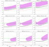 |
Fig. 5. Thomson scattering optical depth of TI zones, plotted against the radial distance from the BH of the mass MBH = 108 M⊙, and shown for three values of magnetic parameters M1, M2, and M3 (from left to right columns), and an accretion rate of ṁ = 0.012, 0.27, and 0.1 (from upper to bottom rows). The photosphere is marked using the green dashed line, temperature minimum with a thick black solid line, thermalization depth (τ * = 1) with a red dotted line. The extent of the thermal instability is presented as a pink-filled area. |
Furthermore, it is produced by radiative processes, such as Comptonization and free-free emission and absorption, being the only cooling processes in the models considered in this paper. Ionization and recombination may influence the extend of TI (Różańska & Czerny 1996), but the final result cannot be analytically predicted. Further computations are needed to show whether ionization or recombination decreases or increases the thermally unstable zone. It’s only for high values of the accretion rate (i.e., higher than 0.2) and in the inner regions of an accretion disk within 20RSchw, the existence of thermally stable warm coronas with classical condition of constant gas pressure is possible. We claim here that in case of the MSD, the condition of thermal stability under constant total namely, gas plus magnetic pressure should be used in order to estimate if the TI zone is frozen into a magnetic field. In a forthcoming paper, we plan to calculate relevant timescales for this kind of radiative cooling in the magnetically supported plasma.
3.4. Random models sample
Our numerical code (GR20) allows us to calculate a huge number of models in a finite time. In order to put constraints on basic observational parameters resulting from our model: temperature of the corona and its optical depth, we have selected results from random distribution of six input parameters for our calculations described in Sect. 2.1, to account for their uncertainty. We use a notation whereby U(a, b) is a random variable with a uniform distribution between a and b and N(μ, σ) is a normal distribution with expected value μ and spread σ. We use a fixed radius R = 6RSchw, while black hole mass, MBH, and accretion rate, Ṁ, (in g s−1) are selected in the way to mimic the distribution of the same quantities in the sample of 51 AGN for which the warm corona was observed (Jin et al. 2012, see section below). The random walk overdoes through the following distribution:


where the expected and spread values were estimated from the observed sample. After running the code and solving the structure, we reject the models that satisfy the radiation pressure criteria described in Sect. 2.4.
We generated a set of models based on random distribution of the global disk parameters described by Eqs. (25) and (26). The vertical structures of all models in the sample are plotted collectively in Fig. 6, with the full sample (upper panels) as well as sample clipped according to the criterion of the density inversion (lower panels) described in Sect. 2.4. The temperature inversion occurs between τ = 0.01 and τ = 30 for all models, with both the magnetic field and accretion rate having a positive effect on the corona depth, as shown in left panels of both rows of Fig. 6. The density follows a rather predictable relation  and the heating rate changes as
  , with small fluctuations due to the opacity.
 |
Fig. 6. Vertical structure of temperature, density and dissipation heating rate defined by Eq. (22) for a sample of models computed according to the method described in Sect. 3.4. The first row shows the complete sample of models, while the second row only shows models that do not exhibit density inversion discussed in Sect. 2.4. Zones where TI occurs are omitted, which produces the gaps that are visible in many models. The color of the line corresponds to the magnetic gradient, q, (red is stronger field, blue is weaker), while the thickness shows the accretion rate ṁ (thicker is higher). The gray vertical lines show the optical depths τ equal to (from left to right): 100, 10, 1, 0.1, and 0.01. |
When we remove the models that do not satisfy our criterion for the density gradient (i.e., moving from the upper to lower panels of Fig. 6), the picture does not change much, but it becomes more complex when we omit the parts of the structure which is thermally unstable (when dlnΛ/dlnT < 0). For the set of models we analyzed, the TI is confined to the area where 10−24 ≤ qh ≤ 10−22 and this does not seem to strongly vary with any of the model parameters we consider. Thus, we can summarize these results according to the following: independently of the model parameters, those associated with the accretion disk or with the magnetic field, the classical TI (under constant gas pressure) is present for magnetically supported disk with radiative processes as Comptonization and free-free emission.
3.5. Observational predictions
As the main outcome of our computations, we obtain values for the warm coronal temperatures and optical depths, which are directly comparable to the measurements reported in the literature. The data analysis concerning warm corona require high resolution, sensitive telescopes to collect enough photons in the soft X-ray energy range around 1 keV. The overall modeling is time consuming and usually one paper is devoted to one source. We have looked at the literature and we chose those sources for which both parameters: warm coronal temperature and its optical depth were measured. The warm corona measurement for the sample of objects has only been presented by Jin et al. (2012), who collected 51 sources. We take all those points into account while comparing to data. In addition we selected measured warm corona parameters of individual sources found in Magdziarz et al. (1998), Page et al. (2004), Mehdipour et al. (2011, 2015), Done et al. (2012), Petrucci et al. (2013), Matt et al. (2014), Middei et al. (2018, 2019), Porquet et al. (2018), Ursini et al. (2018). All data points compared to our model in Sect. 3.5 below, are listed in Table 1.
Observational points from literature compared to our model.
From our random sample of models, we extracted essential parameters as optical depth of the warm corona, its temperature, accretion rate, black hole mass, and magnetic field gradient (all described at the beginning of Sect. 3). The results are shown in Fig. 7, where the random values described in Sect. 3.4 were selected to roughly match the observational points taken from Table 1, in terms of accretion rate and the black hole mass. At the same time, we allowed the magnetic parameters of the disk to vary across a very broad range, namely, from β0 ≈ 103 to β0 ≈ 1. This allows us to scan all possibilities while remaining close to observations in terms of known quantities. Observations are marked on the right side of the figure according to data analyzed in papers listed in Table 1. Some source are reported twice or even more, but it does not matter since we are interested in the general observational trend of the warm corona.
 |
Fig. 7. Parameters of the corona τcor and Tavg determined for a random sample of models are marked by open circles. The size of the points determines the accretion rate and color of the points corresponds to the magnetic field gradient (similar to Fig. 6) given on the right side of the figure. For models where the TI is present, the values of τ and Tavg computed at every point of the instability are displayed by thin lines. In the left panel, all models are shown, while in the right panel, models where the density inversion occurs (see Sect. 2.4) are filtered out. Additionally, data points from the literature are drawn using black markers listed on the right side of the figure. The data points clearly follow TI strips. |
In the left panel of Fig. 7, we include all results of our models by colored open circles, with no limit to radiation pressure or viscous instability (as long as the model has converged). The size of the circle indicates the value of the accretion rate, while its color reflect the value of magnetic field gradient, both given on the right side of the figure. The cloud of points on the τcor–Tavg plane coincide with the observational results, but the range of corona parameters obtained with our numerical code is broader. A clear correlation of magnetic field strength and the accretion rate with resulting corona parameters is seen. Observations follow the models computed for higher accretion rates and moderate magnetic field gradient.
In the right panel of Fig. 7, we removed all the models where the density inversion occurs, which are the models dominated by the radiation pressure and not stabilized by magnetic pressure. We rejected these models because unless convection is present to transfer the energy from the disk, the solution becomes “puffed up” and generally unstable. The models that are removed in this step are mostly models when τcor < 10 or optically thick models with high accretion and low magnetic field. The data points seem to group around the models which do not display TI in the structure of the warm corona, but some of them follow thin lines, which are thermally unstable zones. The distribution among instability strips can be attributed to our choice of the cutoff of the corona base at the temperature minimum. Had it been chosen according to a different criterion, a more shallow and hotter corona would be obtained. The TI might cause the corona to be shallower than the temperature minimum, which could potentially happen at undetermined point in the vertical structure.
To check at which point the vertical structure the data is in line with the model, we took the black hole mass and the accretion rate for each point from Jin et al. (2012) and we ran a corresponding model, assuming constant magnetic parameters of αB = 0.18, η = 0.21 and ν = 1. The global disk parameters were chosen to fall roughly in the middle of the range consistent with the observations. We then proceeded to tune the parameter αB for each model, so that at the optical depth, τcor, the average temperature yields Tavg, with both values taken from the observational data. For some models, it is not possible, but for most (44 objects from the sample of 51), such value of αB does exist. Both fixed-parameter and fine-tuned models are shown in Fig. 8, where different colors display different global parameters for the disk. The observed cases of Tavg versus τcor are marked by filled circles, while the same parameters as an outcome of our adjusted models are given by crosses. Additionally, using solid thin lines, we plot the averaged temperature integrated from the surface down to the local optical depth given on the x-axis of our graph. The thick solid lines display the extensions of thermally unstable zones. The cases displaying high accretion rates (shown at the top) do not indicate TI. It is clear from the figure that tuning the magnetic parameters does not result in any significant change, which means that the fixed values are a good approximation for this set of observations.
 |
Fig. 8. Profiles of averaged temperature versus the optical depth for fine-tune models. The temperature is averaged between the optical depth given by the coordinate of the horizontal axis and the surface of the corona. Thicker lines are overlayed to indicate where the condition for the TI is fulfilled. Circle markers are temperatures and optical depths obtained by Jin et al. (2012). Cross markers indicate the averaged temperature at τcor of a given model. Magnetic parameters are adjusted so that the temperature profile crosses the observational point. Each profile is shifted slightly for a clearer presentation and models are sorted according to the accretion rate, ṁ. |
In most cases, the observed optical depth of the warm corona is shallower than the τcor derived from our model (indicated by crosses in the figure), with the exception of a few models with the lowest accretion rates, where it seems to be deeper than predicted. For a range of models, the location of the warm corona is very coincident with the bottom, rather than the top of the TI, and the locations of the two exhibit some correlation in that range. Above some threshold, our model does not predict the occurrence of the TI, yet the observed optical depth falls short compared to the τcor from our model.
4. Discussion
We computed a sample of models of the disk-corona vertical structure, where both layers are physically bounded by magnetic field heating as well as Compton and free-free cooling. Our approach to the MRI description is parameterized to adjust the results obtained from simulations, as explained in GR20. The warm, optically thick corona is formed self consistently on the top of an accretion disk for the range of global disk and magnetic parameters. In general, the optical depth of the warm corona is larger for a higher accretion rate and a higher magnetization. Nevertheless, the data show that even models of moderate accretion rates can reproduce the observations when the magnetic parameters are adjusted.
Magnetic heating does not remove the classical TI under constant gas pressure seen in regions of high temperatures on the order of 1 keV and high densities on the order of 1012 cm−3, cooled by radiation processes. Interestingly, this kind of TI is created only for Compton and free-free absorption or emission. When magnetic heating with simple description of MRI and recconection is taken into account as a main source of gas heating, the disk becomes dominated by magnetic pressure, which acts as a freezer for the TI zone. In order to check this behavior, a stability parameter should be computed under constant gas plus magnetic pressure. In such a case, classical TI exists with negative slope of temperature versus ionization parameter, but the stability parameter under constant gas plus magnetic pressure is always positive. To prove whether such gas is stable, the timescales for TI frozen into magnetic field should be estimated and we plan to do so in the forthcoming paper. In the all previous approaches to the ionized disk atmospheres, the ionization structure was always solved only up to the depth of the photosphere, namely, to the lower branch, which was stabilized due to atomic cooling and heating. Many papers showing such a stability curve never run the computations deeper in the disk structure where the energy is dissipated. In our approach, the magnetic heating that is generated at each point of a vertical structure of the disk and corona provides additional properties to the normal behavior of the gas, namely: the cold disk temperature increases when going towards the equatorial plane, as explicitly presented in panel a of Fig. 1.
Compton and free-free processes fully account for the extension of stability curve from the hot layers on the corona surface, down to the corona base at τcor. Ionization and recombination may increase the unstable zone, but this should be checked in the future studies. Also, TI may impact the gas evolution on thermal timescales. In the future, time-dependent simulations may show the impact of TI on the warm corona gas.
For all analyzed models, the structure was stable when the isobaric constraint of constant gas plus magnetic pressure was assumed. Of course, such a treatment of a magnetic field only holds true in idealized case, assuming that the field is frozen into matter and there are no significant pressure gradients along the flux tube. If there is a pressure change, the magnetic structure would need to inflate as a whole, without any escape of the matter. Practically, magnetic structures in the corona are tangled and can be considered as pressurized, but open. If a thermal runaway or collapse occurred in a flux tube, matter could be pushed or sucked into the flux tube in order to maintain the pressure equilibrium. In such cases, even in the presence of a strong field, the original criterion of constant gas pressure would hold and strong TI would occur within separate flux tubes, forming prominence-like structures. If we searched for the conditions needed to obtain a uniform, warm corona (and not clumpy prominences), the density n0 (Eq. (15)) would still be a reasonable order-of-magnitude limitation.
4.1. Observations predictions and modeling implications
As we demonstrate in this work, the observations follow our model of a warm corona heated by MRI. All of the data points are in the range T = 0.01–1 keV and τes = 2–50. The coronal temperature appears to be strongly correlated with the coronal magnetic field (in particular, its spatial gradient). The accretion rate, on the other hand, seems to increase the optical depth of the corona, at the slight cost of temperature.
Our numerical model has several weaknesses. The greatest limitation to our model is that it is static and one-dimensional. That implies that the corona assumed must be layer-like, clumpy, and unstable, but optically thick clumps cannot be studied. According to the degree that the models are affected by the thermal instability, in our study we were not able definitively exclude the possibility that the clumpy corona can also reproduce the observations. It is possible that a dynamical model could resolve the issue of a local instability, as long as the overall optically thick disk structure survives.
It is also possible that a thin-disk approximation is not well-suited to the problem, as there is growing evidence that multi-layer accretion where the accretion of disk and corona are decoupled may be more realistic (Lančová et al. 2019; Wielgus et al. 2022). We were not able to treat such an accretion mode with our approach.
Another limitation is that we could not obtain the spectrum from our model. While quantities such as optical depth and temperature can be fitted to spectra and we may compare the values with our model, there is some level of degeneracy and the best way to verify the correctness of our predictions would be to at least compare the spectral parameter Γ, which is the slope of the power law usually fitted to the data.
Despite those limitations, our model has allowed us to determine the location and properties of the TI. That said, we cannot exclude that there is a coincidence of occurrence of TI i our models and the warm corona in nature. One peculiar possibility is that the warm corona could actually be driven by the TI. Instead of one layer, many scatterings through more and less dense areas could be more effective than a single, uniform layer in producing a Comptonization spectrum. More investigations are needed using dynamic models that allow for the unstable, clumpy medium to develop (including the magnetic field as essential part to maintain the physical structure of the clumps) and followed by radiative transfer calculations aimed at proving whether such structures can indeed create warm Comptonization signatures.
If we assume the opposite but (as far as we consider) more likely alternative that the clumpy medium does not contribute to the observed spectrum, another interesting possibility emerges. It could be that the corona exists at the verge of the instability. The new warm matter is constantly inflowing, and once it reaches the unstable conditions, it collapses into clumps that are ejected or (more likely) fall back into the disk core. If the condensation timescale is long compared to the dynamical timescale, the matter could exist at the brink of the instability long enough to continuously Comptonizes the soft photons. This could act as a stabilizing mechanism and explain why the observed properties of the warm corona seem to be clustered in a narrow range of the parameter space. While we cannot distinguish which of these scenarios is closer to the truth, the striking coincidence of the warm corona with TI is hard to overlook.
5. Conclusions
We have clearly demonstrated that magnetic heating can produce a warm and optically thick corona above accretion disk in AGN. Obtained theoretical values of coronal temperatures and optical depths agree with those observed for the best known sources. The magnetic viscosity parameter increases the coronal temperature as well as the optical thickness. Magnetic heating does not remove the local thermal instability of the corona (TI) caused by radiation processes in the warm (∼1.0 keV), and dense (above 1012 cm−3) gas. Classical TI operates for accretion rates lower than 0.1 in Eddington units and does not depend much on magnetic viscosity; nevertheless, it is always the combination of those parameters fully determines instability strip. When magnetic heating is taken into account, stability parameter computed under constant gas plus magnetic pressure is always positive, suggesting that thermally unstable zone in the classical way, becomes a kind of frozen into magnetic field and can produce interesting observational features, including soft X-ray excess.
The case of AGNs differs from that of GBHBs, where TI occurs for ṁ < 0,003 for low αB and ṁ < 0,05 for high αB (GR20). Also, the optical thickness of the warm corona in AGN is relatively higher than in the case of GBHBs by a factor of 5. Interestingly, TI operates only when Compton heating and free-free emission are introduced. It does not require ionization or recombination processes to be included. Nevertheless, we claim here that ionization may influence the extension of the TI zone and we plan to check it in our future work.
Observations follow TI strip of the warm corona in magnetically supported disk. Thermally unstable gas may undergo evolution under thermal timescale, which, in principle, can be computed in our models. Such theoretical timescale should be compared to the variability measurements of soft corona. We plan to do so in the next step of our project. We conclude here that the TI resulting in the gas, which is cooled due to radiation, may be a common mechanism affecting the existence of the warm corona above accretion disks around black holes across different masses. This is confirmed by the fact that we obtained TI in the disk vertical structure in the case of AGNs considered here, as well as in case of GBHB presented in our previous paper (GR20).
Acknowledgments
This research was supported by Polish National Science Center grants No. 2019/33/N/ST9/02804 and 2021/41/B/ST9/04110. We acknowledge financial support from the International Space Science Institute (ISSI) through the International Team proposal “Warm coronae in AGN: Observational evidence and physical understanding”. Software: FORTRAN, Python (Van Rossum & Drake 2009), Sympy (Meurer et al. 2017), LAPACK (Anderson et al. 1990) and GNU Parallel (Tange 2011).
References
- Adhikari, T. P., Różańska, A., Sobolewska, M., & Czerny, B. 2015, ApJ, 815, 83 [NASA ADS] [CrossRef] [Google Scholar]
- Anderson, E., Bai, Z., Dongarra, J., et al. 1990, in Proceedings of the 1990 ACM/IEEE Conference on Supercomputing, Supercomputing ’90 (Los Alamitos, CA, USA: IEEE Computer Society Press), 2 [Google Scholar]
- Ballantyne, D. R. 2020, MNRAS, 491, 3553 [NASA ADS] [CrossRef] [Google Scholar]
- Begelman, M. C. 2006, ApJ, 643, 1065 [NASA ADS] [CrossRef] [Google Scholar]
- Begelman, M. C., Armitage, P. J., & Reynolds, C. S. 2015, ApJ, 809, 118 [Google Scholar]
- Bianchi, S., Guainazzi, M., Matt, G., Fonseca Bonilla, N., & Ponti, G. 2009, A&A, 495, 421 [NASA ADS] [CrossRef] [EDP Sciences] [Google Scholar]
- Crummy, J., Fabian, A. C., Gallo, L., & Ross, R. R. 2006, MNRAS, 365, 1067 [Google Scholar]
- Done, C., Davis, S. W., Jin, C., Blaes, O., & Ward, M. 2012, MNRAS, 420, 1848 [Google Scholar]
- Field, G. B. 1965, ApJ, 142, 531 [Google Scholar]
- García, J. A., Kara, E., Walton, D., et al. 2019, ApJ, 871, 88 [CrossRef] [Google Scholar]
- Gierliński, M., & Done, C. 2004, MNRAS, 349, L7 [Google Scholar]
- Gronkiewicz, D., & Różańska, A. 2020, A&A, 633, A35 [NASA ADS] [CrossRef] [EDP Sciences] [Google Scholar]
- Haardt, F., & Maraschi, L. 1991, ApJ, 380, L51 [Google Scholar]
- Henyey, L. G., Forbes, J. E., & Gould, N. L. 1964, ApJ, 139, 306 [NASA ADS] [CrossRef] [Google Scholar]
- Janiuk, A., & Czerny, B. 2011, MNRAS, 414, 2186 [NASA ADS] [CrossRef] [Google Scholar]
- Jiang, Y.-F., Stone, J. M., & Davis, S. W. 2014, ApJ, 784, 169 [NASA ADS] [CrossRef] [Google Scholar]
- Jin, C., Ward, M., Done, C., & Gelbord, J. 2012, MNRAS, 420, 1825 [Google Scholar]
- Kato, S., Fukue, J., & Mineshige, S. 2008, Black-Hole Accretion Disks – Towards a New Paradigm – [Google Scholar]
- Keek, L., & Ballantyne, D. R. 2016, MNRAS, 456, 2722 [CrossRef] [Google Scholar]
- Krolik, J. H., McKee, C. F., & Tarter, C. B. 1981, ApJ, 249, 422 [NASA ADS] [CrossRef] [Google Scholar]
- Lančová, D., Abarca, D., Kluźniak, W., et al. 2019, ApJ, 884, L37 [CrossRef] [Google Scholar]
- Laor, A., Fiore, F., Elvis, M., Wilkes, B. J., & McDowell, J. C. 1994, ApJ, 435, 611 [NASA ADS] [CrossRef] [Google Scholar]
- Laor, A., Fiore, F., Elvis, M., Wilkes, B. J., & McDowell, J. C. 1997, ApJ, 477, 93 [Google Scholar]
- Lightman, A. P., & Eardley, D. M. 1974, ApJ, 187, L1 [Google Scholar]
- Madau, P. 1988, ApJ, 327, 116 [NASA ADS] [CrossRef] [Google Scholar]
- Magdziarz, P., Blaes, O. M., Zdziarski, A. A., Johnson, W. N., & Smith, D. A. 1998, MNRAS, 301, 179 [NASA ADS] [CrossRef] [Google Scholar]
- Matt, G., Marinucci, A., Guainazzi, M., et al. 2014, MNRAS, 439, 3016 [NASA ADS] [CrossRef] [Google Scholar]
- Mehdipour, M., Branduardi-Raymont, G., Kaastra, J. S., et al. 2011, A&A, 534, A39 [NASA ADS] [CrossRef] [EDP Sciences] [Google Scholar]
- Mehdipour, M., Kaastra, J. S., Kriss, G. A., et al. 2015, A&A, 575, A22 [NASA ADS] [CrossRef] [EDP Sciences] [Google Scholar]
- Meurer, A., Smith, C. P., Paprocki, M., et al. 2017, PeerJ Comput. Sci., 3, e103 [CrossRef] [Google Scholar]
- Middei, R., Bianchi, S., Cappi, M., et al. 2018, A&A, 615, A163 [NASA ADS] [CrossRef] [EDP Sciences] [Google Scholar]
- Middei, R., Bianchi, S., Petrucci, P. O., et al. 2019, MNRAS, 483, 4695 [NASA ADS] [CrossRef] [Google Scholar]
- Page, K. L., Schartel, N., Turner, M. J. L., & O’Brien, P. T. 2004, MNRAS, 352, 523 [CrossRef] [Google Scholar]
- Pessah, M. E., & Psaltis, D. 2005, ApJ, 628, 879 [NASA ADS] [CrossRef] [Google Scholar]
- Petrucci, P.-O., Paltani, S., Malzac, J., et al. 2013, A&A, 549, A73 [NASA ADS] [CrossRef] [EDP Sciences] [Google Scholar]
- Petrucci, P. O., Ursini, F., De Rosa, A., et al. 2018, A&A, 611, A59 [NASA ADS] [CrossRef] [EDP Sciences] [Google Scholar]
- Petrucci, P. O., Gronkiewicz, D., Rozanska, A., et al. 2020, A&A, 634, A85 [NASA ADS] [CrossRef] [EDP Sciences] [Google Scholar]
- Piconcelli, E., Jimenez-Bailón, E., Guainazzi, M., et al. 2005, A&A, 432, 15 [NASA ADS] [CrossRef] [EDP Sciences] [Google Scholar]
- Porquet, D., Reeves, J. N., Matt, G., et al. 2018, A&A, 609, A42 [NASA ADS] [CrossRef] [EDP Sciences] [Google Scholar]
- Pounds, K. A., Stanger, V. J., Turner, T. J., King, A. R., & Czerny, B. 1987, MNRAS, 224, 443 [NASA ADS] [CrossRef] [Google Scholar]
- Różańska, A. 1999, MNRAS, 308, 751 [CrossRef] [Google Scholar]
- Różańska, A., & Czerny, B. 1996, Acta Astron., 46, 233 [NASA ADS] [Google Scholar]
- Różańska, A., Czerny, B., Życki, P. T., & Pojmański, G. 1999, MNRAS, 305, 481 [CrossRef] [Google Scholar]
- Różańska, A., Malzac, J., Belmont, R., Czerny, B., & Petrucci, P.-O. 2015, A&A, 580, A77 [NASA ADS] [CrossRef] [EDP Sciences] [Google Scholar]
- Salvesen, G., Simon, J. B., Armitage, P. J., & Begelman, M. C. 2016, MNRAS, 457, 857 [Google Scholar]
- Shakura, N. I., & Sunyaev, R. A. 1973, A&A, 24, 337 [NASA ADS] [Google Scholar]
- Shakura, N. I., & Sunyaev, R. A. 1976, MNRAS, 175, 613 [NASA ADS] [CrossRef] [Google Scholar]
- Shibazaki, N., & Hōshi, R. 1975, Prog. Theor. Phys., 54, 706 [CrossRef] [Google Scholar]
- Szuszkiewicz, E., & Miller, J. C. 1997, MNRAS, 287, 165 [NASA ADS] [CrossRef] [Google Scholar]
- Tange, O. 2011, The USENIX Mag., 36, 42 [Google Scholar]
- Ursini, F., Petrucci, P. O., Matt, G., et al. 2018, MNRAS, 478, 2663 [NASA ADS] [CrossRef] [Google Scholar]
- Van Rossum, G., & Drake, F. L. 2009, Python 3 Reference Manual (Scotts Valley, CA: CreateSpace) [Google Scholar]
- Walter, R., & Fink, H. H. 1993, A&A, 274, 105 [NASA ADS] [Google Scholar]
- Walton, D. J., Nardini, E., Fabian, A. C., Gallo, L. C., & Reis, R. C. 2013, MNRAS, 428, 2901 [NASA ADS] [CrossRef] [Google Scholar]
- Wielgus, M., Lančová, D., Straub, O., et al. 2022, MNRAS, 514, 780 [CrossRef] [Google Scholar]
All Tables
All Figures
|
Fig. 1. Vertical structure of an accretion disk for our CM model versus z in cm measured from disk mid-plane (z = 0) up to the surface (right side of the figure panels), and for three different sets of magnetic parameters ranging from the strongest (M1, as a yellow line) to the weakest (M3, as a black line) magnetic field, and listed in the box below the figure. The local temperature, ionization parameter (Eqs. (17) and (20)), and stability parameter (Eq. (18)) are plotted in the top row, while pressures, fluxes relative to the total dissipated flux, and heating rate are plotted in the bottom row, respectively. In addition, the value of |
| In the text | |
|
Fig. 2. Temperature structure of an accretion disk for our CM model versus ionization parameter (left panel), stability parameter (middle panel) and all three pressure components (right panel). Gas pressure structure is given by dashed-dotted line, magnetic pressure by dashed line, and radiation pressure by dotted line. Three models of different magnetization are defined as in Fig. 1, and given by colors: M1 – black, M2 – green, and M2 – red. At each panel, the position of temperature minimum is clearly indicated by a triangle of the same color. Gray dotted line in the middle panel marks the limit of negative value of stability parameter. Thick solid lines in the right panel cover values of pressure and temperature for which classical stability parameter (under constant gas pressure) is negative. |
| In the text | |
|
Fig. 3. Properties of the warm corona on the accretion rate-magnetic viscosity parameter plane. All models have been calculated for MBH = 108 M⊙ and R = 6 RSchw. Upper panels show: a) average temperature, Tavg, of the corona in keV (colors) and optical depth of the base of the warm corona τcor (contours); b) Ξ (colors) and magnetic pressure parameter β (contours) both at τcor; and c) number density nH in cm−3 (colors) at τcor and total column density Σ in g cm−2 (contours). Dotted contour here shows where dΣ/dṁ = 0. Bottom panels display: d) yavg parameter of the warm corona at the thermalization zone, namely, τ* = 1 (colors), and at the base of the corona, τcor (contours); e) fraction of radiative energy produced by the corona f (colors) and the maximum value of magnetic field gradient q (contours); and f) the minimum value of ℒrad throughout the disk height (colors) and Thomson optical depth, τmin, for which it occurs (contours), green areas are stable disks, whereas magenta areas indicate thermal instability in the corona, the gray dotted line corresponds to ℒrad = 0. In all panels, the dark contour indicates the parameter sub-space affected by the density inversion. |
| In the text | |
|
Fig. 4. Properties of the warm corona on accretion rate-radius plane given in units of RSchw. All models have been calculated for MBH = 108 M⊙, and magnetic parameters are corresponding M1 (left), M2 (middle), and M3 (right) panel columns with values given under Fig. 1. Upper panels display average temperature Tavg of the corona in keV (colors) and optical depth of the base of the warm corona τcor (contours). Dotted contours at upper panels indicate where ℒrad = 0 under constant gas pressure. Bottom panels show number density nH in cm−3 (colors) at τcor and total column density Σ in g cm−2 (contours). Dotted contours at bottom panels show where dΣ/dṁ = 0. Dark contours in case of M3 model, indicate the parameter sub-space affected by the density inversion. |
| In the text | |
|
Fig. 5. Thomson scattering optical depth of TI zones, plotted against the radial distance from the BH of the mass MBH = 108 M⊙, and shown for three values of magnetic parameters M1, M2, and M3 (from left to right columns), and an accretion rate of ṁ = 0.012, 0.27, and 0.1 (from upper to bottom rows). The photosphere is marked using the green dashed line, temperature minimum with a thick black solid line, thermalization depth (τ * = 1) with a red dotted line. The extent of the thermal instability is presented as a pink-filled area. |
| In the text | |
|
Fig. 6. Vertical structure of temperature, density and dissipation heating rate defined by Eq. (22) for a sample of models computed according to the method described in Sect. 3.4. The first row shows the complete sample of models, while the second row only shows models that do not exhibit density inversion discussed in Sect. 2.4. Zones where TI occurs are omitted, which produces the gaps that are visible in many models. The color of the line corresponds to the magnetic gradient, q, (red is stronger field, blue is weaker), while the thickness shows the accretion rate ṁ (thicker is higher). The gray vertical lines show the optical depths τ equal to (from left to right): 100, 10, 1, 0.1, and 0.01. |
| In the text | |
|
Fig. 7. Parameters of the corona τcor and Tavg determined for a random sample of models are marked by open circles. The size of the points determines the accretion rate and color of the points corresponds to the magnetic field gradient (similar to Fig. 6) given on the right side of the figure. For models where the TI is present, the values of τ and Tavg computed at every point of the instability are displayed by thin lines. In the left panel, all models are shown, while in the right panel, models where the density inversion occurs (see Sect. 2.4) are filtered out. Additionally, data points from the literature are drawn using black markers listed on the right side of the figure. The data points clearly follow TI strips. |
| In the text | |
|
Fig. 8. Profiles of averaged temperature versus the optical depth for fine-tune models. The temperature is averaged between the optical depth given by the coordinate of the horizontal axis and the surface of the corona. Thicker lines are overlayed to indicate where the condition for the TI is fulfilled. Circle markers are temperatures and optical depths obtained by Jin et al. (2012). Cross markers indicate the averaged temperature at τcor of a given model. Magnetic parameters are adjusted so that the temperature profile crosses the observational point. Each profile is shifted slightly for a clearer presentation and models are sorted according to the accretion rate, ṁ. |
| In the text | |
Current usage metrics show cumulative count of Article Views (full-text article views including HTML views, PDF and ePub downloads, according to the available data) and Abstracts Views on Vision4Press platform.
Data correspond to usage on the plateform after 2015. The current usage metrics is available 48-96 hours after online publication and is updated daily on week days.
Initial download of the metrics may take a while.