| Issue |
A&A
Volume 632, December 2019
|
|
|---|---|---|
| Article Number | A64 | |
| Number of page(s) | 9 | |
| Section | The Sun | |
| DOI | https://doi.org/10.1051/0004-6361/201936822 | |
| Published online | 28 November 2019 | |
Observational signatures of the third harmonic in a decaying kink oscillation of a coronal loop
1
Centre for Fusion, Space and Astrophysics, Department of Physics, University of Warwick, CV4 7AL Coventry, UK
e-mail: This email address is being protected from spambots. You need JavaScript enabled to view it.
2
Max-Planck-Institut für Sonnensystemforschung, Justus-von-Liebig-Weg 3, 37077 Göttingen, Germany
3
Centre for Mathematical Plasma Astrophysics, Mathematics Department, KU Leuven, Celestijnenlaan 200B bus 2400, 3001 Leuven, Belgium
Received:
1
October
2019
Accepted:
28
October
2019
Abstract
Aims. An observation of a coronal loop standing kink mode is analysed to search for higher harmonics, aiming to reveal the relation between different harmonics’ quality factors.
Methods. Observations of a coronal loop were taken by the Atmospheric Imaging Assembly (AIA) of the Solar Dynamics Observatory (SDO). The loop’s axis was tracked at many spatial positions along the loop to generate time series data.
Results. The distribution of spectral power of the oscillatory transverse displacements throughout the loop reveals the presence of two harmonics, a fundamental at a period of ∼8 min and its third harmonic at ∼2.6 min. The node of the third harmonic is seen at approximately a third of the way along the length of the loop, and cross correlations between the oscillatory motion on opposing sides of the node show a change in phase behaviour. The ratio of periods P1/3P3 was found to be ∼0.87, indicating a non-uniform distribution of kink speed through the loop. The quality factor for the fundamental mode of oscillation was measured to be ∼3.4. The quality factor of the third harmonic was measured for each spatial location and, where data was reliable, yielded a value of ∼3.6. For all locations, the quality factors for the two harmonics were found to agree within error as expected from 1d resonant absorption theory. This is the first time a measurement of the signal quality for a higher harmonic of a kink oscillation has been reported with spatially resolved data.
Key words: magnetohydrodynamics (MHD) / Sun: corona / Sun: magnetic fields / Sun: oscillations / waves
© ESO 2019
1. Introduction
Coronal seismology uses the modelling of magnetohydrodynamic (MHD) waves in plasma structures and the comparison with observations for the diagnostics of the plasma (see reviews by Nakariakov et al. 2016; De Moortel & Nakariakov 2012; Andries et al. 2009, and references therein). The interpretation of observations of transversely oscillating coronal loops as fast kink modes is one commonly performed example (Nakariakov et al. 1999), which relies on the theory of the eigenmodes in a magnetic cylinder (Zaitsev & Stepanov 1982; Edwin & Roberts 1983). These well-used models for linear waves are described by dispersion relations obtained for uniform, equilibrium models of very thin, axisymmetric, long, and straight tubes. Often the approximations considered are good enough to extract useful information about the plasma via seismology, particularly when estimating the physical parameters averaged across the entire loop.
Standing kink oscillations in coronal loops have been extensively observed with a typical period, Pkink, of several minutes (c.f. statistical studies by Goddard et al. 2016; Nechaeva et al. 2019); both period and damping time have been observed to scale linearly with the loop length L. Through these observations the seismological estimation of the (local) magnetic field can be made, which is often difficult to determine directly (Nakariakov & Ofman 2001). However this magnetic field value relies on estimates of the density and a spatial average of Alfvén speed along the entire loop.
The use of multiple harmonics (fundamental and its overtones) can provide more information for seismology thus allowing one to match the observed dispersion with that predicted by theory (Andries et al. 2009). Further, it is natural to expect the occurrence of higher parallel harmonics when a kink oscillation is impulsively excited, as is predominantly the case (Zimovets & Nakariakov 2015). In principle, by observing multiple different harmonics the dispersion relation used for seismological inversion can be verified. Conversely if the theoretical dispersion relation is assumed to be correct, one can attribute any observational departure from the theoretical dispersion relation to modifications, such as density stratification. In practice, this is often done through the comparison of the measured harmonic periods P1/nPn, that is, the ratio of the fundamental period P1 to n times that of the nth harmonic, Pn. For a dispersionless oscillation (i.e. when each harmonic has the same phase speed Ckink), the ratio P1/nPn is unity for all n. Any departure from unity provides information about dispersion along the loop. This dispersion is assumed to be from the spatial variation of kink speed along the loop, which can be used to probe the plasma structure (Jain & Hindman 2012).
The comparison of different wave modes to provide further seismological information was first demonstrated in Andries et al. (2005) by using observations of a loop arcade hosting higher harmonics as reported in Verwichte et al. (2004). The detected departure from unity of P1/2P2 was attributed to the density stratification along the coronal loop and a value for the density scale height was determined; the process is also analytically described in McEwan et al. (2006, 2008). More recently, Guo et al. (2015) and Pascoe et al. (2016a) both spatially resolved the fundamental and second harmonic of two distinct standing kink oscillations using observations with the Atmospheric Imaging Assembly (AIA) on board the Solar Dynamics Observatory (SDO), utilising spectral techniques and comparing oscillation phase behaviour of the loop legs. Kupriyanova et al. (2013) detected multiple periodicities in a flaring loop’s microwave emission, and they used a comparison with the dispersion equation for oscillation eigenmodes in a straight homogeneous cylinder and further spatial information to support the conclusion of a multi-harmonic standing kink mode. Similar conclusions were reached for a flaring loop seen in the hard X-ray and microwave wavelengths in Inglis & Nakariakov (2009). In both cases the mechanism for how kink modes modulate microwave emission is non-trivial, making it difficult to perform seismology confidently.
Additional information for the determination of plasma parameters from seismology has been shown to reside in the oscillation damping profile (Aschwanden et al. 2003). The main mechanism by which trapped kink modes are thought to damp away is resonant absorption (Ruderman & Roberts 2002). Kink modes couple to torsional, incompressible Alfvén modes that reside in a resonant shell within the cylinder, transferring energy from the transverse motion of the cylinder into plasma motions within. In this model for the damping, the damping time τn is proportional to the period Pn (Ofman & Aschwanden 2002). Thus the quality factor (signal quality) of the oscillation τ/P is the same for each harmonic n, which is determined by the physical properties of the loop including its transverse density profile (c.f. Eq. (1), Pascoe et al. 2016a). This should hold true regardless of dispersion modifying the period of the nth harmonic from its expected value P1/n, since the damping time should change accordingly.
In this paper we present the first measurement of the period ratio to the fundamental and the damping behaviour of a kink oscillation’s third harmonic. The coronal loop kink oscillation is described in Sect. 2. The co-existence of the fundamental and third harmonic standing modes is verified by using their spatial and phase distributions, as explained in Sect. 3, and by employing a bandpass filter to separate the third harmonic signal. The separate components are independently fitted by damped sinusoids, and their resulting parameter values through the loop are explored in Sect. 4. In Sect. 5 the period ratio between and quality factors of the two harmonics is compared. The discussions and conclusions are presented in Sect. 6.
2. Observation
This work is motivated by Pascoe et al. (2016b, 2017) in which the event used for the following analysis is referred to as Loop #2. The coronal loop of interest was observed on 26 May 2012 off the north easterly limb of the Sun in SDO/AIA EUV 171 Å, using data with cadence 12 s and AIA pixel size of 0.6 arcsec. The loop is associated with NOAA active region 11484, which by this time has rotated out of view. The loop is observed from side-on, such that the plane of the loop is perpendicular to the plane of sky. Another well-contrasted loop is seen perpendicular to the loop of interest, apparently crossing (in the field of view) about half-way up the loop of interest’s leg, meaning data from this region is unavailable. The loop of interest in Fig. 1 has its axis approximately denoted by the dashed line. Its length is estimated as 162 ± 3 Mm. At approximately 20:38 UT the bundle of loops (of which this loop is part) is restructured. This appears to coincide with the emanation of a blast wave visible in 171 Å. As part of this restructuring, one footpoint of the loop of interest appears to “jump” from approximately (890, 320) arcsec to (900, 290) arcsec, although the precise locations of the footpoint are subjective. Consequently the loop sways about its (new) equilibrium position with decaying amplitude for about one hour, after which the loop disappears out of the 171 Å passband. This event constitutes a standing kink oscillation, referenced in the kink oscillation catalogue compiled in Nechaeva et al. (2019) as Event 27 Loop 1.
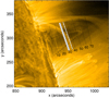 |
Fig. 1. SDO/AIA 171 Å image of the loop, 2012 May 26 20:50 UT. Every other slit location used to extract time-distance data from is indicated. The slit nearest the limb is indexed 1, the slit nearest the apex is indexed 60, as indicated by the labelled slits with thicker lines. The white hashed areas denote noisy slits where data was not good enough to get reliable time series. |
For the loop of interest, data can only be obtained for one loop leg. Therefore 70 straight slits with a length of 100 pixels were created perpendicular to the loop plane – these are denoted by solid black lines in Fig. 1. To reduce noise, each slit is averaged over a 5 pixel width perpendicular to the slit. Slits indexed 16 to 59 were of good enough quality to take into further analysis. For later plots, the slit index value is understood to be a spatial coordinate, ranging from just above the limb (on the loop leg near the footpoint) at slit 16, up to the loop apex which corresponds to slit 59. For each usable slit, time-distance maps were generated, some examples of which may be seen in Fig. 2. The start and end times for these plots are 20:34 UT and 21:42 UT respectively. For each time-distance map, the loop axis was fitted at each instance of time to yield time series data following the procedure outlined in Pascoe et al. (2016b). Slits 27, 28, 29, and 34 were too noisy to take into further analysis, predominantly caused by signal from the edges of another loop overlapping the loop of interest.
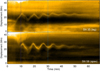 |
Fig. 2. Example time-distance maps from slit 35 (top) situated about half way up the loop leg, and slit 58 (bottom) near the loop apex. The overplotted white dotted line shows the fitted time series data. Each time distance map was averaged over 5 pixels perpendicular to the slit. The blue vertical lines denote where data was cut before the spectral analysis and fitting. In real time these correspond to 20:44 UT and 21:04 UT. |
3. Verification of multiple harmonics
3.1. Spectral analysis
To investigate the loop oscillation, we first examine its spectrum. At each slit we consider the wavelet transform of its time series. Figure 3 shows one such wavelet power spectrum for a slit part-way up the length of the loop. The wavelet plot clearly shows a strong spectral component between 7 and 8 min. Examining the time series further, a low amplitude departure from a harmonic signal is seen superimposed on the first few periods. This is realised in the wavelet plot as a feature at approximately a minute period, lasting for the first 10 min or so and with a far lower spectral power than the component at 8 min. This is consistent with the features of a rapidly damped third harmonic, in line with the result reported in Pascoe et al. (2016b).
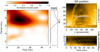 |
Fig. 3. Left: morlet wavelet plot of the time series data corresponding to slit 26. Middle: global wavelet spectrum, normalised to its maximum value. The period of maximal global wavelet power for this slit’s time series is found to be 7.28 min. Right top: SDO/AIA image, rotated for reader’s convenience, on which the loop midplane (dashed line) and slit position (solid line) is overlaid. Right bottom: time-distance map for this slit (zoomed), from which the time series is extracted. |
It can be seen in Fig. 2 that the loop displacement at some spatial locations appears fairly harmonic, such as near the apex, while other locations show more anharmonic behaviour, especially in the first period of oscillation. Therefore to check if this spectral component truly is a third harmonic, we investigate its spatial distribution along the loop. A third harmonic would be expected to have a node one third along the length of the loop, a point which should be visible from the AIA camera’s perspective. To observe this node, the global wavelet spectrum (GWS) of each time series is calculated and plotted against height along loop (slit number) in Fig. 4. Only data between 10 and 30 min (as indicated on Fig. 2) was used for this and subsequent analysis, motivated by the short duration of the spectral component at 3 min seen in Fig. 3 and the expectation of rapid damping. The GWS is advantageous over a traditional Fourier decomposition due to the presence of distinct spectral components lasting different lengths of time. The Fourier spectrum may not show significant spectral peaks where there are overtones, due to their limited time duration compared to the Fourier basis vector (complex exponential). The alternative spectral decomposition of GWS can address this shortcoming since wavelet spectral analysis sacrifices the ability to distinguish two spectral peaks at very similar frequencies (which may be resolvable using Fourier decomposition) in order to gain information about when the spectral components are present. The dominant period in Fig. 4 is 7.87 min, calculated as the peak of the sum of GWS amplitude over all slits. This periodicity exists over all slits considered but decreasing in amplitude towards the loop footpoint, that is to say having a single antinode at the apex. This matches expectations of the fundamental standing kink mode, and with this interpretation for a loop of this length (162 Mm), using the formula Ckink ≈ 2L/Pkink yields a reasonable estimate of the averaged loop kink speed Ckink ≈ 0.69 Mm s−1.
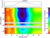 |
Fig. 4. Two–dimensional distribution of spectral amplitude estimated from the Global Wavelet Spectrum per slit against period and slit number. Top: amplitude summed across all slits shows a peak at ∼7.87 min. The hashed regions correspond to slits where the data was not good enough to get reliable time series, predominantly caused by an overlapping loop. |
Also visible in Fig. 4 is a band of spectral amplitude for most slits at a period of approximately 3 min, lower amplitude than the dominant period and with an apparent dip at approximately slit 51. This matches expectations of a third harmonic, which is to say having a period of approximately 7.87/3 = 2.6 min and a node existing one third of the way along the loop’s axis. Due to the perspective seeing the loop side on, this node would appear at rsin(π/3)/r ≈ 0.87 of total loop height r, which matches the approximate position of slit 51/60 ≈ 0.85. The amplitude of the shorter period spectral component is an order of magnitude smaller than the fundamental, and is just discernible in the GWS. This is consistent with the excitation of kink modes by an external perturbation in simulations by Pascoe & De Moortel (2014, e.g. see Fig. 2).
3.2. Phase behaviour
To investigate the phase behaviour of the short period component, a bandpass filter is employed to separate this component from the dominant signal. The filter used was an ideal step function in Fourier space allowing periods between two and four minutes, setting all other frequencies to zero. Testing between filtering using the Fourier transform and filtering based on the wavelet transform showed no significant difference, so the more widely used Fourier filter was used. Filters of different shapes – ideal step function, Gaussian, Hanning, Hamming – were also tested and none had any discernible advantage, and so the rectangular function was used to maximise spectral resolution. Zero padding the time series prior to the Fourier transform was used to minimise edge effects. As was the case for creating the GWS data, the time series used here were cut to the first 20 min. This was motivated by the short time duration of the spectral component seen in wavelet plots such as Fig. 3.
To examine the phase behaviour along the loop, reliance on fitting the data is not necessary. An alternative empirical method is to calculate the correlation between a chosen slit’s time series and all others. A positive correlation close to +1 would indicate the oscillation is in phase at the spatial locations corresponding to the slit indices. If the correlation is 0 this would indicate either the oscillation is π/2 out of phase or there is no signal amplitude at one (or both) slits. A negative correlation close to −1 would imply the oscillation is in perfect antiphase at the two spatial locations. Thus plotting this correlation against slit index gives a picture of how the oscillation phase varies across the loop, whilst the choice of reference slit location determines against which phase the others are measured. This method makes no assumption about the precise shape or period of the oscillatory components, making it more amenable to real data than fitting artificially exact sinusoids. In the ideal situation, comparison between loop legs may be performed (for example in Duckenfield et al. 2018), however useful information can be extracted even when considering only one loop leg.
For the fundamental mode of oscillation, the entire loop oscillates in phase and thus a plot of correlation value against slit number appears flat for all choices of reference slit. For the third harmonic one expects two nodes to occur along the loop, across which there should be a phase shift. For this observation’s point of view, only one node would be visible. An illustrative example for the n = 3 case is given in the top panel of Fig. 5. Data from the same side of the node are perfectly correlated with each other, switching to perfect anti-correlation when cross-correlated with data from the opposite side of the node. At the node of the third harmonic the correlations pass through zero (since there is no oscillatory signal in one time series). The correlations with respect to a point further down the loop leg, that is to say the opposite side of the node at slit 51, show the same behaviour but reflected. This pattern is seen when looking at cross correlations with respect to the apex (black), and also for cross correlations with respect to the apex (red) but reflected. The node position is also obvious as the point at which both the red and black curve intersect each other.
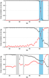 |
Fig. 5. Correlation values calculated when a slit’s time series is cross correlated with a reference slit. Cross correlation values with the reference slit near the apex (slit 59) are shown in red, and on the same plot, the cross correlation values with the reference slit near the leg (slit 19) are shown in black. The region marked by blue highlights where the amplitude of the third harmonic is low, and data is not trustworthy. Top: expected correlations, calculated using synthetically generated time series for a perfect third harmonic signal, incorporating the side on perspective and only showing one leg (as is the case for the real data). Middle: synthetically generated time series consisting of a fundamental mode, a third harmonic and (coloured) noise. This synthetic signal also underwent the same bandpass filter as was used on the data. Bottom: correlation plot calculated from data. The existence of the node of the third harmonic is clearly seen. |
In the middle panel of Fig. 5, the introduction of noise and bandpass filtering have had some effects. The cross correlations have deviated away from +1 and −1, the swap of the red and black curves happens over a larger number of slits, and there is some asymmetry between them. All these features are also seen in the real data in the bottom panel of Fig. 5. There is more slit-to-slit variation than seen in the data, however this is probably because the real data were averaged over 5 pixels before forming time series. This averaging has a spatial scale of the same order as the distance between slits (∼3 arcsec), and so overlap between adjacent slits may act as a smoothing.
Referring to the bottom panel of Fig. 5 we can see some of the expected phase behaviour of the filtered oscillation signal manifested in the cross-correlation data. There is a transition near slit 51, where the node of the third harmonic is expected, although this appears shifted. It is worth remembering the small-to-non-existent signal amplitude around this location, which means that the correlation is dominated by noise. This is compounded by the fact that there is uncertainty exactly where the node should be since we do not know exactly the loop length, height etc, so the “true” node could lie anywhere nearby. The most negative correlation is −0.3. For real data, correlations very near −1 are unfeasible, and this oscillatory signal is on the edge of detectability, with low signal to noise and additional filtering required. Further, the side on perspective means that there are few slits available for analysis between the third harmonic node and the apex, all of which are potentially contaminated by additional noise, from integrating through more of the loop. Despite the shortcomings when applied to real data, the fact that the harmonic node behaviour is seen in the bandpass filtered data provides evidence of the third harmonic.
4. Determining oscillation parameters
To further confirm the spectral components’ veracity as kink oscillation harmonics n = 1 and n = 3 and to compare the two, we consider the behaviour of the oscillation’s parameters along the loop. The displacement of the loop at each slit location is modelled as a damped sinuosidal function in the form
 (1)
(1)
A time-dependent background trend is not included. Although the loop displacements have a slight change in equilibrium position between start and end, fitting this end necessarily changes the frequency spectrum of the resultant time series in a subjective way. For this data the trend is sufficiently close to a single mean value that useful results can be obtained without removing the trend, even at the level of the small amplitude third harmonic. The loop length does not visibly change within the time of interest. Therefore to keep the results reproducible and reduce the number of parameters to estimate, only a mean value is fitted to each slit. Two example slits are shown in Fig. 6. Although the difference between the peaks of the calculated sinusoids and the peaks visible on the time distance maps do vary slightly with time, these differences are indeed minor. As we see no obvious period drift in the wavelet plots such as Fig. 3, the period is not allowed to vary in time in the fitting, but is fitted independently for different slit positions.
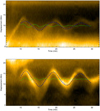 |
Fig. 6. Time distance maps overlaid with sinusoids calculated using the MAP parameters output by the MCMC sampling for that respective slit. The sinusoid corresponding to n = 1 is in blue, the sinusoid corresponding to n = 3 is in green, and their sum is shown by the dashed black line. The average displacement of the loop for each slit has been added so the curves line up with time distance map behind it. Top: slit 26 as shown in Fig. 3. The summed curve clearly deviates from a pure sinusoid as per the time distance map behind it, as a result of the third harmonic. Bottom: slit 59 at the apex. Despite being an antinode for the third harmonic, the summed curve does not deviate far from a pure sinusoid due to the large amplitude of the n = 1 component. |
We choose to allow the amplitude to only evolve in time through a Gaussian decaying term. It is known both Gaussian and exponential envelopes could occur as the damping envelope at different times and/or under different conditions. For example an exact kink eigenmode would decay exponentially. In general both observations and simulations indicate an oscillation damping profile may best be approximated via a switch between the two (Pascoe et al. 2016a). For the purposes of this work however, the introduction of further free parameters to the fitting – as would be required to include both modes of damping – detracts from the clarity of following a single parameter along the loop. A single damping parameter, though potentially underestimating the mode coupling rate, is enough to compare how the damping is different between harmonics and between different spatial locations along the loop. A Gaussian decay term is chosen because the simultaneous excitation of multiple harmonics implies the exciter is not an exact kink eigenmode, and supported by the results seen in Pascoe et al. (2016b, e.g. Fig. 2).
For this model, Bayesian inference and Markov chain Monte Carlo sampling is used to determine the parameter values that best describe the data in the same manner as described in Pascoe et al. (2016b). As a result, in the following analysis we consider the best fit to be that with the maximum a posteriori probability (MAP) estimate returned for the parameters amplitude A, phase ϕ, period P and damping time τ. Uniformly distributed priors are used, with upper and lower limits covering the expected range of reasonable values (for example n = 3 period between two and four minutes). The MCMC sampling is independently applied at each slit location, building a picture of how the oscillation parameters vary along the loop. The credible intervals, seen in Figs. 7 and 8 as grey shaded regions, are estimated as the 95% confidence level of the marginalised posterior distribution for that particular parameter.
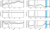 |
Fig. 7. Resulting parameters from MCMC sampling to describe the unfiltered data (corresponding to the fundamental n = 1 mode) (left column), and to describe the filtered data (corresponding to the third harmonic n = 3) (right column). The parameters are amplitude (top), period (middle), and damping time (bottom). The black diamonds show the MAP parameter value from the MCMC sampling, and its credible interval is shaded light grey for each slit. The hashed regions correspond to slits where the data was not good enough to get reliable time series, predominantly caused by an overlapping loop. The blue region denotes the approximate node for the third harmonic, where amplitude is small and data is not to be trusted. |
In this paper the oscillation parameters for the two spectral components are fitted separately. In Pascoe et al. (2017) for each oscillation, a single time series is tested against models comprised of a simultaneous fundamental mode, higher harmonics, a trend, and a decay-less component. The relationship between harmonics is fixed for each compared model. This approach is not appropriate in this paper because we are interested in measuring each harmonic’s oscillation parameters separately. To keep the interpretation of our results – how an individual parameter changes with spatial location – simple, we choose to keep the number of parameters as small as possible and use Bayesian inference to determine which set of parameters is most probable. Therefore we use the bandpass filter and fitting to a simple model to directly compare the harmonics, whilst employing other additional techniques to confirm the harmonics’ existence.
4.1. Parameters of the fundamental mode
To investigate the n = 1 component, the unfiltered (original) time series data is used, as opposed to shorter signal minus filtered data, because the amplitude of the longer period component is so dominant that it was judged the effects of filtering would have a more detrimental effect to the fitting than the superposition of the shorter period component. The resulting MAP parameters from the MCMC sampling for each slit are displayed in the left hand column of Fig. 7.
The fitted amplitude is seen to grow steadily with slit index, that is to say approaching the apex, as expected. The amplitude of the fundamental mode is constant near the apex, as the dependence is sine-like. The fitted period is approximately the same for all slits at an average of 7.8 min, although at the very apex the fitted period drops to about 7.6 min. The damping time is approximately the same for all slits, averaging at 26 min. There are wide credible intervals for most slits on the damping time, particularly down the loop leg, due to the difficulty of its estimation on so few cycles and the ambiguity of the precise damping profile at work (for a detailed discussion see Pascoe et al. 2016b). In line with common sense, the credible intervals seen on the fitted amplitude, period and damping time all decrease with slit index. This results from the amplitude growing with height for the fundamental mode, hence increasing the oscillation signal-to-noise. This can be seen explicitly in Fig. 6, where the amplitude of the blue curve for slit 26 is smaller than that for slit 59 (apex), as expected.
4.2. Parameters of the third harmonic
To investigate the n = 3 harmonic, the bandpass filtered and truncated data are fitted in the same manner as before using Eq. (1), and displayed in the right hand column of Fig. 7. This data is far noisier with a lower signal-to noise ratio, and so fitting with such functions everywhere is optimistic. Despite this, the amplitude MAP values follow the pattern expected: growing amplitude with height until about slit index 40, after which the amplitude drops to near zero at slit 51 (expected node), then beginning to grow again. The (initial) amplitudes are generally less than half that for the fundamental even without accounting for any phase shift, indicating the third harmonic has lower amplitude than the fundamental. The period MAP values output by the MCMC sampling have an average of 3.0 min, which agrees with the period seen with enhanced spectral amplitude in Fig. 4. Unexpectedly there appears a slight period difference between the apex and the loop leg for the third harmonic. For an oscillation satisfying a linear wave equation with no steady flows in cylindrical coordinates, one expects the temporal behaviour to be the same everywhere spatially, or in other words we expect the period to be the same at the apex as down the legs. This holds even when the wave speed (CA) is a function of space. We are motivated to assume the wave equation dictates the observed loop motion because of the great successes of coronal seismology, and because the loop does not exhibit other signatures of non-linear behaviour. It is true that a steady flow would introduce another term in the wave equation that could introduce some variation in temporal behaviour, however in this observation no clear siphon flows were seen, and spectral observations of similar coronal loops imply the flows are of insufficient velocities to have a significant effect. Since we expect the period is constant, this period difference is attributed to spurious additional signal, be it from random noise, leakage from the filtered n = 1 signal, or some effect involving both loop legs along the line of sight. In any case the period difference should be disregarded. Looking at the bottom right plot of Fig. 7, the n = 3 damping time MAP values are moderately constant, although two regions with large credible intervals stand out – one at the node (slit 51), and another nearest the apex. For the first, we expect the fitting on slits near the node to break down due to low amplitude and hence signal-to-noise, as indicated by the blue region. Regarding the second wide range of credible damping values, being near the apex implies something else could be contaminating the signal there. A similar increase in error is visible near the apex in the amplitude values, whilst the periods’ credible intervals are so small they appear unaffected.
When MCMC sampling different realisations of the model specified in Eq. (1), it is necessary to compute the phase ϕ. The values calculated for the filtered (n = 3) data broadly follow a similar shape to the correlations seen in the bottom panel of Fig. 5, but are extremely noisy. There is leakage from the filtering, in which some signal attributed to the fundamental mode is redistributed into the filtered data. This leakage grows with height, since its origin has a greater amplitude near the apex. The sampling does a good job estimating the parameter values that best describe the amplitude, period, and damping time despite this additional noise, resulting in well confined histograms of the samples of these parameters’ posterior probability density functions. However the phase parameter is especially sensitive to this noise, and reporting its MAP values would not do a good job of demonstrating this variability. The phase behaviour for the n = 3 data is discussed in Sect. 3.2, so in the interest of clarity the phase MAP values are not included.
5. Comparison of harmonics
5.1. P1/3P3 ratio
A small departure from unity of the P1/3P3 ratio is seen in Fig. 8, lying between 0.8 and 1.0 for all slits. The average value of P1/3P3 across all slits is 0.87. It should be noted that since a bandpass filter was applied to make visible the n = 3 signal, this would force the ratio to lie between 0.66 and 1.27 even for no signal. However because the ratio values calculated are far from these boundaries the filtering is not believed to limit the results. Separate calculations of this ratio for different spatial locations are used as separate measurements of the same quantity, and not to investigate how this quantity changes along the loop. Despite this ratio being closer to 1 for positions near the apex than for positions down the leg, we still interpret this oscillation as a collective standing mode of the entire loop. The variation in fact originates from the measure of n = 3 period described above in Sect. 4, and is thus disregarded.
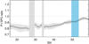 |
Fig. 8. Ratio of fitted period of the fundamental to 3 times the fitted period for the third harmonic, for each slit. Unity is marked with a dashed grey line. The blue region denotes the approximate range in which the n = 3 node exists. The grey region shows an estimate of the credible intervals for this ratio. These are derived using the credible intervals on the periods measured separately for the two harmonics, and propagated through the formula P1/3P3 in the usual manner for errors. |
As outlined in the introduction, this departure from unity may be attributed to the third harmonic experiencing a different (large-scale) spatial average of kink speed to that experienced by the fundamental, predominantly determined by the plasma parameters at each harmonic’s antinodes (Jain & Hindman 2012). That the ratio is less than unity implies that the kink speed experienced by the third harmonic is on average faster than that for the fundamental.
One mechanism that could be responsible for changing kink speed along the loop, such that it is slower at the loop apex than further down the legs, is density stratification. If this were the case, we could estimate the density stratification height H from the measured departure from unity. To illustrate this, we use the functional form of the stratification considered by Andries et al. (2005), Safari et al. (2007) to find
 (2)
(2)
Using the average value of the P1/3P3, measured to be 0.87, and the loop length of L = 162 ± 3 Mm yields a reasonable value of H = 32 Mm. This value is very sensitive to small changes in period ratio however. To demonstrate, using the smallest measured period ratio of 0.80 coupled with L = 159 Mm yields a lower limit of H = 18 Mm, whereas using the largest measured period ratio of 0.97 coupled with L = 165 Mm yields an upper limit of H = 150 Mm. Nonetheless this exercise illustrates in principle the benefits of detecting higher harmonics.
There are other effects that may explain the departure from unity of P1/3P3: magnetic field (cross section) variation, curvature, ellipticity, or siphon flows. Discussion on these effects may be found in Andries et al. (2009). Other more esoteric cases such as temperature difference effects (Orza et al. 2012) could potentially play a role. It should also not be forgotten that even the ideal kink modes in a cylindrical geometry are slightly dispersive due to the waveguide, though the effect should be small (Edwin & Roberts 1983). The dispersion effect on long wavelength modes has therefore previously been taken to be negligible for unstratified loops (Van Doorsselaere et al. 2007; McEwan et al. 2006). To compare the relative likelihood of several different models explaining a non-uniform kink speed, one may use a Bayesian statistics methodology (for example see Arregui et al. 2013). In principle such comparative analysis using information from both oscillation harmonics is appropriate for this sort of observation, as the Bayesian framework allows progressively more information to be introduced through its prior distributions, however such an analysis is not presented here.
5.2. Comparison of quality factors
Figure 9 shows the first attempt to compare quality factors τi/Pi for different oscillation harmonics. The average quality factor of all slits from fitting of the original time series (taken to be the quality factor for the fundamental harmonic n = 1) was found to be τ1/P1 = 3.4. The credible intervals found on the quality factors for the fundamental decrease with spatial index, as expected from higher amplitude signal nearer the loop apex having increased signal to noise ratio.
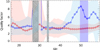 |
Fig. 9. Signal quality factors calculated from fitting original (n = 1) data for each slit (red), and from fitting the bandpass filtered data in blue (n = 3). Diamonds show the quality factor value, and error estimates calculated using the credible intervals for τi and Pi propagated through standard error formula are shown in red for n = 1, and blue for n = 3. The purple region denotes the region in which the n = 3 node lies. |
Quality factors for the third harmonic n = 3 are estimated from the fitting of the bandpass filtered time series with damped sinusoids. For slits 15 to 45 along the leg, sufficiently below the third harmonic node, the average quality factor is τ3/P3 = 3.6. The average quality factor for all slits is 5.5, however this value is severely affected by uncertainty on the larger slit indices as can be seen on Fig. 9. It is also clear that the uncertainty on the quality factors for the filtered data become substantially larger near slit 51. This also conforms to common sense, since this is the spatial location of the node of the third harmonic. The credible intervals reduce towards the apex, only to balloon at the very highest locations. The quality factor itself is larger at higher slit numbers, caused by the slight period difference making the denominator (period) smaller. As discussed above this effect is most likely not real. For all slits, the quality factor calculated for n = 3 agrees with the quality factor for n = 1 within the levels of uncertainty. The conclusion that may be drawn is that the quality factors for the fundamental compared to those from the third harmonic agree within error along the whole loop.
6. Discussion and conclusions
In this paper we have investigated the transverse oscillation of a coronal loop and shown it to contain two periods of oscillation, 7.8 min and 3.0 min. These are attributed to be the fundamental standing kink mode and its third harmonic. Evidence for this includes a spectral decomposition of the oscillation at all points along the loop with the global wavelet transform, where the two periods are seen distinctly with a period ratio of approximately 3. A node for the higher frequency component can also be seen at the expected spatial location one third along the loop, accounting for line of sight. A bandpass filter – formed of an ideal step function between two and four minutes – allows us to separate out the signal for the third harmonic. Cross correlations of the filtered data confirm the phase behaviour as changing across the node as expected. Fitting the original data and the bandpass filtered data with damped sinusoids at many points along the loop gives estimates for the oscillation parameters throughout the loop, for both frequency components. These also display the spatial dependence of amplitude and phase expected for the fundamental mode of oscillation (n = 1) and its third harmonic (n = 3). Examining the fitted parameters of period and damping time for both harmonics, the ratio of periods P1/3P3 exhibits a slight departure from unity at 0.87, and the quality factors for both harmonics agree within error, agreeing with resonant absorption theory.
It is worth noting that the period measured from the maximum global wavelet amplitude summed over all loops was 7.9 min, which is consistent with the value of 7.7 min measured for the same oscillation in Pascoe et al. (2016b). We have shown here that the period is consistent throughout the observable length of the loop, rather than relying on fitting the oscillation profile at a single spatial location. Only by analysing multiple spatial positions such as in Pascoe et al. (2016a), and investigating the phase behaviours between them can claims of higher harmonics be convincingly made. Relying on the modelling a single time series leaves one susceptible to the choice of spatial location, particularly with respect to observing multiple harmonics. As an example, for this observation if one considered only slit 51 (the node for the third harmonic), one might incorrectly conclude the oscillation contains only one frequency. Similar circumstances would occur if only tracking a loop’s apex, since a second harmonic would have its node there and thus presents little signal to be analysed. The technique outlined in this work, using information of phase and amplitude from across the whole loop, is less susceptible to spatially local biases. This technique would also be ideal for locating antinode positions, which has previously been used for seismology (Guo et al. 2015).
It is interesting that the oscillation does not exhibit signatures of the second harmonic as strongly as for the third harmonic, which damps away faster. This absence of the second harmonic implies the perturbation was symmetric about the apex, as in the simulations in Pascoe & De Moortel (2014). This is in contrast to the observation in Pascoe et al. (2016a), where the second harmonic was excited by an eruption that clearly affected one leg more than the other and so was strongly asymmetric. We can be confident the third harmonic was not excited by some non-linear cascade or evolution, because we would expect there to be some inertial period in which the non-linearity grows, or in other words see the amplitude grow and then decrease. Yet it may be seen in Fig. 7 that the third harmonic has its highest amplitude at the beginning of the oscillation, and both modes of oscillation appear to begin at the same time. Together these make the simultaneous excitation of the fundamental and third harmonic the simplest explanation for the observed behaviour. The fundamental mode being most strongly excited implies the spatial scale of the perturbation was comparable with the loop length, kdriver ≥ k1. Because the driver does not coincide with the first harmonic we also get the third harmonic which is also symmetric about the apex. It is also possible that the temporal profile of the driver could influence the generation of higher harmonics, since an impulsive driver localised in space and time is broadband in k − ω space and allows a wide range of frequencies to be excited. This was recently demonstrated for the case of propagating sausage modes (Goddard et al. 2019). Either way we might expect the fifth harmonic to also be present with an amplitude about an order of magnitude weaker than the third harmonic, though that would be undetectable because of its very small period of oscillation, damping rate, and amplitude.
In this observation, it was shown that (within error) the quality factors for the third harmonic and the fundamental agree across the whole loop. This is as expected for a loop whose transverse density profile and density contrast does not vary longitudinally along the loop, since resonant absorption relates the quality factor to loop density contrast, its transverse density profile and the width of the inhomogeneous layer in which resonant absorption is maximised (Ruderman & Roberts 2002). It is also expected that uniform density stratification would approximately preserve this relation between damping time and period (Dymova & Ruderman 2006). However there is information about different density profiles at different heights embedded in the comparison of quality factors for different harmonics, because the damping rate is strongly dependent on transverse density profile (Pascoe et al. 2017). If there was a longitudinal variation in density profile (and/or density contrast), different harmonics would experience different quality factors. The fact that we do not see much difference between quality factors (within our resolution), nor does the loop cross section in AIA appear to vary between the apex and the loop leg, implies the loop’s density profile and density contrast are fairly constant throughout the loop. This is believed to be the first time such comparison has been done, so the potential of such comparisons of quality factors is still largely unknown. This would naturally call into question the following: whether the resonant absorption rates would be affected differently for various types of harmonics, and whether this could be observed by using similar observations as those presented in this paper.
Overall it may be seen that spatial resolution of oscillation harmonics and their parameters may be useful for information about the coronal loop structure. In particular the differences between harmonics could lead to more informative comparisons between observed dispersion and theory, potentially shedding a light on things previously hidden such as the internal density structure of the loop. Higher harmonics are not uncommon in solar coronal loops oscillations, and the detection of higher harmonics in the ubiquitous decay-less oscillations also means such seismological tools demonstrated here could be used more widely than just flaring loops. It is imperative that more theoretical work is carried out to this end, particularly examination of the effect of spatially varying transverse density profile upon different harmonics’ resonant absorption.
Acknowledgments
This work was supported by the British Council via the Institutional Links Programme (Project 277352569 “Seismology of Solar Coronal Active Regions”), the STFC consolidated grant ST/L000733/1. DJP was supported by the GOA-2015-014 (KU Leuven) and the European Research Council (ERC) under the European Union’s Horizon 2020 research and innovation programme (grant agreement No 724326). CRG was supported by ERC Synergy grant WHOLE SUN 810218.
References
- Andries, J., Arregui, I., & Goossens, M. 2005, ApJ, 624, L57 [NASA ADS] [CrossRef] [Google Scholar]
- Andries, J., van Doorsselaere, T., Roberts, B., et al. 2009, Space Sci. Rev., 149, 3 [NASA ADS] [CrossRef] [Google Scholar]
- Arregui, I., Asensio Ramos, A., & Díaz, A. J. 2013, ApJ, 765, L23 [NASA ADS] [CrossRef] [Google Scholar]
- Aschwanden, M. J., Nightingale, R. W., Andries, J., Goossens, M., & Van Doorsselaere, T. 2003, ApJ, 598, 1375 [NASA ADS] [CrossRef] [Google Scholar]
- De Moortel, I., & Nakariakov, V. M. 2012, Philos. Trans. R. Soc. London A: Math. Phys. Eng. Sci., 370, 3193 [Google Scholar]
- Duckenfield, T., Anfinogentov, S. A., Pascoe, D. J., & Nakariakov, V. M. 2018, ApJ, 854, L5 [NASA ADS] [CrossRef] [Google Scholar]
- Dymova, M. V., & Ruderman, M. S. 2006, A&A, 457, 1059 [NASA ADS] [CrossRef] [EDP Sciences] [Google Scholar]
- Edwin, P. M., & Roberts, B. 1983, Sol. Phys., 88, 179 [NASA ADS] [CrossRef] [Google Scholar]
- Goddard, C. R., Nisticò, G., Nakariakov, V. M., & Zimovets, I. V. 2016, A&A, 585, A137 [NASA ADS] [CrossRef] [EDP Sciences] [Google Scholar]
- Goddard, C. R., Nakariakov, V. M., & Pascoe, D. J. 2019, A&A, 624, L4 [NASA ADS] [CrossRef] [EDP Sciences] [Google Scholar]
- Guo, Y., Erdélyi, R., Srivastava, A. K., et al. 2015, ApJ, 799, 151 [NASA ADS] [CrossRef] [Google Scholar]
- Inglis, A. R., & Nakariakov, V. M. 2009, A&A, 493, 259 [NASA ADS] [CrossRef] [EDP Sciences] [Google Scholar]
- Jain, R., & Hindman, B. W. 2012, A&A, 545, A138 [NASA ADS] [CrossRef] [EDP Sciences] [Google Scholar]
- Kupriyanova, E. G., Melnikov, V. F., & Shibasaki, K. 2013, Sol. Phys., 284, 559 [NASA ADS] [CrossRef] [Google Scholar]
- McEwan, M. P., Donnelly, G. R., Díaz, A. J., & Roberts, B. 2006, A&A, 460, 893 [NASA ADS] [CrossRef] [EDP Sciences] [Google Scholar]
- McEwan, M. P., Díaz, A. J., & Roberts, B. 2008, A&A, 481, 819 [NASA ADS] [CrossRef] [EDP Sciences] [Google Scholar]
- Nakariakov, V. M., & Ofman, L. 2001, A&A, 372, L53 [NASA ADS] [CrossRef] [EDP Sciences] [Google Scholar]
- Nakariakov, V. M., Ofman, L., Deluca, E. E., Roberts, B., & Davila, J. M. 1999, Science, 285, 862 [NASA ADS] [CrossRef] [PubMed] [Google Scholar]
- Nakariakov, V. M., Pilipenko, V., Heilig, B., et al. 2016, Space Sci. Rev., 200, 75 [NASA ADS] [CrossRef] [Google Scholar]
- Nechaeva, A., Zimovets, I. V., Nakariakov, V. M., & Goddard, C. R. 2019, ApJS, 241, 31 [NASA ADS] [CrossRef] [Google Scholar]
- Ofman, L., & Aschwanden, M. J. 2002, ApJ, 576, L153 [NASA ADS] [CrossRef] [Google Scholar]
- Orza, B., Ballai, I., Jain, R., & Murawski, K. 2012, A&A, 537, A41 [NASA ADS] [CrossRef] [EDP Sciences] [Google Scholar]
- Pascoe, D. J., & De Moortel, I. 2014, ApJ, 784, 101 [NASA ADS] [CrossRef] [Google Scholar]
- Pascoe, D. J., Goddard, C. R., & Nakariakov, V. M. 2016a, A&A, 593, A53 [NASA ADS] [CrossRef] [EDP Sciences] [Google Scholar]
- Pascoe, D. J., Goddard, C. R., Nisticò, G., Anfinogentov, S., & Nakariakov, V. M. 2016b, A&A, 589, A136 [NASA ADS] [CrossRef] [EDP Sciences] [Google Scholar]
- Pascoe, D. J., Anfinogentov, S., Nisticò, G., Goddard, C. R., & Nakariakov, V. M. 2017, A&A, 600, A78 [NASA ADS] [CrossRef] [EDP Sciences] [Google Scholar]
- Ruderman, M. S., & Roberts, B. 2002, ApJ, 577, 475 [NASA ADS] [CrossRef] [Google Scholar]
- Safari, H., Nasiri, S., & Sobouti, Y. 2007, A&A, 470, 1111 [NASA ADS] [CrossRef] [EDP Sciences] [Google Scholar]
- Van Doorsselaere, T., Nakariakov, V. M., & Verwichte, E. 2007, A&A, 473, 959 [NASA ADS] [CrossRef] [EDP Sciences] [Google Scholar]
- Verwichte, E., Nakariakov, V. M., Ofman, L., & Deluca, E. E. 2004, Sol. Phys., 223, 77 [NASA ADS] [CrossRef] [Google Scholar]
- Zaitsev, V. V., & Stepanov, A. V. 1982, Sov. Astron. Lett., 8, 132 [NASA ADS] [Google Scholar]
- Zimovets, I. V., & Nakariakov, V. M. 2015, A&A, 577, A4 [NASA ADS] [CrossRef] [EDP Sciences] [Google Scholar]
All Figures
|
Fig. 1. SDO/AIA 171 Å image of the loop, 2012 May 26 20:50 UT. Every other slit location used to extract time-distance data from is indicated. The slit nearest the limb is indexed 1, the slit nearest the apex is indexed 60, as indicated by the labelled slits with thicker lines. The white hashed areas denote noisy slits where data was not good enough to get reliable time series. |
| In the text | |
|
Fig. 2. Example time-distance maps from slit 35 (top) situated about half way up the loop leg, and slit 58 (bottom) near the loop apex. The overplotted white dotted line shows the fitted time series data. Each time distance map was averaged over 5 pixels perpendicular to the slit. The blue vertical lines denote where data was cut before the spectral analysis and fitting. In real time these correspond to 20:44 UT and 21:04 UT. |
| In the text | |
|
Fig. 3. Left: morlet wavelet plot of the time series data corresponding to slit 26. Middle: global wavelet spectrum, normalised to its maximum value. The period of maximal global wavelet power for this slit’s time series is found to be 7.28 min. Right top: SDO/AIA image, rotated for reader’s convenience, on which the loop midplane (dashed line) and slit position (solid line) is overlaid. Right bottom: time-distance map for this slit (zoomed), from which the time series is extracted. |
| In the text | |
|
Fig. 4. Two–dimensional distribution of spectral amplitude estimated from the Global Wavelet Spectrum per slit against period and slit number. Top: amplitude summed across all slits shows a peak at ∼7.87 min. The hashed regions correspond to slits where the data was not good enough to get reliable time series, predominantly caused by an overlapping loop. |
| In the text | |
|
Fig. 5. Correlation values calculated when a slit’s time series is cross correlated with a reference slit. Cross correlation values with the reference slit near the apex (slit 59) are shown in red, and on the same plot, the cross correlation values with the reference slit near the leg (slit 19) are shown in black. The region marked by blue highlights where the amplitude of the third harmonic is low, and data is not trustworthy. Top: expected correlations, calculated using synthetically generated time series for a perfect third harmonic signal, incorporating the side on perspective and only showing one leg (as is the case for the real data). Middle: synthetically generated time series consisting of a fundamental mode, a third harmonic and (coloured) noise. This synthetic signal also underwent the same bandpass filter as was used on the data. Bottom: correlation plot calculated from data. The existence of the node of the third harmonic is clearly seen. |
| In the text | |
|
Fig. 6. Time distance maps overlaid with sinusoids calculated using the MAP parameters output by the MCMC sampling for that respective slit. The sinusoid corresponding to n = 1 is in blue, the sinusoid corresponding to n = 3 is in green, and their sum is shown by the dashed black line. The average displacement of the loop for each slit has been added so the curves line up with time distance map behind it. Top: slit 26 as shown in Fig. 3. The summed curve clearly deviates from a pure sinusoid as per the time distance map behind it, as a result of the third harmonic. Bottom: slit 59 at the apex. Despite being an antinode for the third harmonic, the summed curve does not deviate far from a pure sinusoid due to the large amplitude of the n = 1 component. |
| In the text | |
|
Fig. 7. Resulting parameters from MCMC sampling to describe the unfiltered data (corresponding to the fundamental n = 1 mode) (left column), and to describe the filtered data (corresponding to the third harmonic n = 3) (right column). The parameters are amplitude (top), period (middle), and damping time (bottom). The black diamonds show the MAP parameter value from the MCMC sampling, and its credible interval is shaded light grey for each slit. The hashed regions correspond to slits where the data was not good enough to get reliable time series, predominantly caused by an overlapping loop. The blue region denotes the approximate node for the third harmonic, where amplitude is small and data is not to be trusted. |
| In the text | |
|
Fig. 8. Ratio of fitted period of the fundamental to 3 times the fitted period for the third harmonic, for each slit. Unity is marked with a dashed grey line. The blue region denotes the approximate range in which the n = 3 node exists. The grey region shows an estimate of the credible intervals for this ratio. These are derived using the credible intervals on the periods measured separately for the two harmonics, and propagated through the formula P1/3P3 in the usual manner for errors. |
| In the text | |
|
Fig. 9. Signal quality factors calculated from fitting original (n = 1) data for each slit (red), and from fitting the bandpass filtered data in blue (n = 3). Diamonds show the quality factor value, and error estimates calculated using the credible intervals for τi and Pi propagated through standard error formula are shown in red for n = 1, and blue for n = 3. The purple region denotes the region in which the n = 3 node lies. |
| In the text | |
Current usage metrics show cumulative count of Article Views (full-text article views including HTML views, PDF and ePub downloads, according to the available data) and Abstracts Views on Vision4Press platform.
Data correspond to usage on the plateform after 2015. The current usage metrics is available 48-96 hours after online publication and is updated daily on week days.
Initial download of the metrics may take a while.