| Issue |
A&A
Volume 632, December 2019
|
|
|---|---|---|
| Article Number | A92 | |
| Number of page(s) | 8 | |
| Section | The Sun | |
| DOI | https://doi.org/10.1051/0004-6361/201936728 | |
| Published online | 10 December 2019 | |
Investigating the nature of the link between magnetic field orientation and proton temperature in the solar wind
1
Institute for National Astrophysics (INAF) – Institute for Space Astrophysics and Planetology (IAPS), Via Fosso del Cavaliere 100, 00133 Rome, Italy
e-mail: raffaella.damicis@inaf.it
2
Italian Space Agency (ASI), Via del Politecnico snc, 00133 Rome, Italy
Received:
18
September
2019
Accepted:
29
October
2019
Solar wind fluctuations are a mixture of propagating disturbances and advected structures that transfer into the interplanetary space the complicated magnetic topology present at the basis of the corona. The large-scale interplanetary magnetic field introduces a preferential direction in the solar wind, which is particularly relevant for both the propagation of the fluctuations and their anisotropy and for the topology of the structures advected by the wind. This paper focusses on a particular link observed between angular displacements of the local magnetic field orientation from the radial direction and values of the proton temperature. In particular, we find that observations by Helios and Wind show a positive correlation between proton temperature and magnetic field orientation. This is especially true within Alfvénic wind characterized by large-amplitude fluctuations of the background field orientation. Moreover, in the case of Wind, we found a robust dependence of the perpendicular component of the proton temperature on the magnetic field angular displacement. We interpret this signature as possibly due to a physical mechanism related to the proton cyclotron resonance. Finally, by simulating the sampling procedure of the proton velocity distribution function (VDF) of an electrostatic analyzer, we show that the observed temperature anisotropy is not due to instrumental effects.
Key words: solar wind / magnetic fields / methods: data analysis / turbulence / Sun: heliosphere / plasmas
© ESO 2019
1. Introduction
The Helios in-situ measurements have shown unambiguously that the proton temperature ratio T⊥/T∥, within fast wind streams is typically larger than unity and could reach values larger than T⊥/T∥ = 3 at a distance of 0.3 AU from the Sun (Marsch et al. 1982), suggesting strong local ion heating. When the heliocentric distance increases, this ratio tends to decrease down to values around unity at 1 AU. The temperature anisotropy found in the core of the proton velocity distribution (VDF; Marsch et al. 1982), as well as the preferential heating and acceleration of minor ions (see review by Marsch 2006), suggest that a coupling between the magnetic energy of the fluctuations and the kinetic energy of the ions is at work. In this regard, Alfvén-cyclotron waves are thought to play a relevant role through the resonant wave–particle interactions in the heating and acceleration of the solar corona (Zhang et al. 2005) and solar wind (see review by Marsch 2006, and references therein) and, have been invoked in the literature to explain temperature anisotropy in favor of the component perpendicular to the local magnetic field direction.
Bourouaine et al. (2010) showed that temperature anisotropy depends on the power density of transverse magnetic field fluctuations, corroborating the idea that Alfvén waves play a crucial role. Bruno et al. (2006) noted that there is a positive correlation between the angle the magnetic field forms with a fixed direction, say the average background field direction (defined as the angular displacement with respect to that direction) and temperature, T. Bruno et al. (2004) first studied the time behavior of the vector displacement between each magnetic field instantaneous direction and an arbitrary fixed direction which was chosen to be the direction of the first vector of the time series. The choice of the fixed direction is arbitrary and does not change the result of the analysis. In the same paper, Bruno et al. (2004) also defined an angular displacement as the angle this instantaneous direction forms with the fixed direction. It is important to note that the vector and angular displacements provide more information about the vector difference between two vectors at a given scale. Indeed, as shown in Bruno et al. (2004), the vector displacement is obtained as the contribution of two components: small-amplitude and high-frequency fluctuations superimposed on a sort of larger-amplitude low-frequency background structure. Thus, this angle is sensitive to both propagating Alfvénic fluctuations and advected structures (e.g., flux tubes), the two main ingredients of solar wind turbulence. However, the Alfvénic component largely dominates on the nonpropagating structures within the fast wind and in the Alfvénic slow streams studied in our analysis as shown by large values of cross-helicity or of v − b correlation coefficient. This is why this angle can be used to study the relationship, if any, between temperature and magnetic field orientation, although this link must be regarded as qualitative rather than quantitative. In particular, we would expect that an increase in large-amplitude noncompressive magnetic field fluctuations is related to an increase in large directional fluctuations of the background field orientation (and so large θBR), and corresponds to an increase in temperature, T. However, some caution must be taken since data reduction can artificially introduce this correlation when the proton temperature is not obtained from canonical moment calculation of the three-dimensional (3D) proton VDF but rather from the radial component of the total temperature after integration on azimuthal and polar angles, as we discuss below.
Bruno et al. (2006) suggested that the relationship between θBR and T may be due to continuous local generation of high-frequency Alfvén ion-cyclotron waves from low-frequency Alfvén waves through magnetohydrodynamics (MHD) turbulent cascade (e.g., Tu et al. 1984): energy cascades from the largest energy-containing eddies to the high-frequency region of the spectrum where wave–particle interactions energize the ions at scales comparable to those typical of protons (Marsch 2012). The consequent effect of this interaction is a steepening of the spectral index which marks the beginning of the dissipation range (Denskat et al. 1983) or, in other words, the beginning of the frequency range where kinetic effects must be taken into account. It has also been reported (Bruno et al. 2014) that the spectral slope at the beginning of the kinetic range shows high variability and a tendency to be steeper within the trailing edge of the fast streams where the speed and the Alfvénic character of the fluctuations are higher, and to be flatter within the subsequent slow wind. The value of the spectral index depends on the power associated to the fluctuations within the inertial range; the higher the power the steeper the slope, suggesting that there must be some response of the dissipation mechanism which becomes more efficient whenever the energy transfer rate along the inertial range increases (see also D’Amicis et al. 2019a). Nevertheless, it was shown that steeper indices belong to hotter wind samples, supporting the idea that steeper spectral indices in the dissipation range imply greater heating rates (Leamon et al. 1998).
On the other hand, there is a conspicuous number of different theoretical approaches to explain the heating of the space plasma with particular reference to the proton temperature anisotropy (Wang et al. 2006; Wu & Yoon 2007; Nariyuki et al. 2010; Verscharen & Marsch 2011; Dong 2014; Voitenko & Goossens 2004; Chandran et al. 2010; Bourouaine & Chandran 2013; Osman et al. 2011; Dmitruk et al. 2004; Vasquez & Hollweg 2001, among others) and not based on the cyclotron resonant interaction, and there is not yet a general consensus on one of them.
In addition to the debate over theory, there is also an experimental aspect that has to be considered. At present, the complete measurement of the full 3D proton VDF in space performed by Helios takes a rather long time compared to, for example, the inverse of the local gyrofrequency, and it has been suggested (Verscharen & Marsch 2011) that this might influence the correct evaluation of the temperature anisotropy favoring the perpendicular component especially when the proton VDF is sampled in the presence of large-amplitude Alfvénic fluctuations like those observed by Helios in fast wind streams close to the sun (Bruno et al. 1985). In other words, a slow sampling procedure might produce a sort of smearing effect which would introduce an artificial temperature anisotropy.
In the present paper we analyze and compare Helios observations at 0.3 AU with Wind observations at 1 AU. We search in both databases for a clear relationship between field orientation computed at the smallest available scale (40.5 s) and plasma temperature. Moreover, we simulate the sampling procedure of the proton VDF followed by an electrostatic analyzer looking for possible instrumental effects. We conclude that while the Helios database is dominated by effects produced by noncanonical plasma data reduction which introduces artificial correlations between the two parameters above, results based on Wind data show a genuine link between the same parameters. In particular, we find that the perpendicular temperature depends on the amplitude of angular displacements of the magnetic field from the radial direction.
2. Data analysis
Alfvénic fluctuations are believed to play a relevant role in heating and accelerating the solar wind. They are characterized by large-amplitude magnetic field fluctuations related to large directional fluctuations of the background field orientation for a quasi-constant magnetic field intensity with respect to a given fixed direction, such as for example the radial direction. The angle the magnetic field forms with the radial direction, indicated as θBR, can then can be used to study magnetic field fluctuations as described in the introduction. Following preliminary results by Bruno et al. (2006), we focus this section on the study of the relationship between θBR and temperature, at different radial distances, using data from Helios and Wind. We would expect that an increase in θBR corresponds to an increase in temperature although this behavior has to be intended as qualitative rather than quantitative.
2.1. Helios observations
To examine the relationship between θBR and the proton temperature, T, in a statistically robust manner as suggested by Bruno et al. (2006), we started analyzing Helios data at the perihelion. We select Helios 2 observations at 40.5 s resolution using data from the plasma experiment E1 (Rosenbauer et al. 1977) and from the magnetic field experiment E3 (described by Scearce et al. 1975; Mariani et al. 1978). We focus on a time interval spanning heliocentric distances around the perihelion passage (from 0.356 to 0.293 AU) from day 101 to day 107 of year 1976. This represents the best example so far of a fast wind stream showing large-amplitude Alfvénic fluctuations in the solar wind close to the Sun. Proton data were downloaded from the NASA website CDAWeb where the contribution of the alpha particle population has been removed.
Figure 1 shows Helios 2 perihelion passage characterized by a transition from a slow to a fast wind stream, thus providing the opportunity to compare the behavior of different solar wind conditions. In the hypothesis of Alfvén waves playing a role in solar wind heating, we would expect a different degree of correlation between magnetic field orientation and proton temperature for the two solar wind types. Presently, the two winds are characterized by a different Alfvénic content, with fast wind being more Alfvénic than slow wind (Bruno & Carbone 2013).
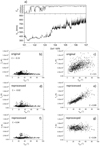 |
Fig. 1. Helios 2 at 0.3 AU. Panel a: bulk speed, Vsw (lower plot), and the v − b correlation coefficient at 1 h scale, Cvb (upper plot). Panels b and c: scatter plots of TR (as derived with Eq. (1)) and θBR for an interval of slow wind (left) and fast wind (right), respectively, using data from NASA website CDAWeb (https://cdaweb.sci.gsfc.nasa.gov), indicated as original. Panels d and e: analogous to panels b and c, respectively, for data from the Space Sciences Laboratory University of California (Berkeley) dataset (http://helios-data.ssl.berkeley.edu/data/), indicated as reprocessed. We show also the scatter plots of the total temperature T vs. θBR referring to reprocessed data in panels f and g. Panels b–g: we report also the value of the linear correlation coefficient, C, between TR (or T) and θBR, in the zoomed time intervals. |
Panel a of Fig. 1 shows the solar wind speed profile, Vsw, (lower plot) along with the v − b correlation coefficient (upper plot) between the z components of magnetic field, b, and velocity, v in the RTN (Radial, Tangential, Normal) coordinate system, indicated as Cvb which is computed at 1 h scale, well within the Alfvénic range, using a sliding window. Here, Cvb is a measure of the degree of Alfvénicity. The fast wind stream from about day 103.15 to the end of the interval is characterized by a high v − b correlation, Cvb being equal to 0.9 on average. The time interval preceding it on the other hand is marked by an alternation of small portions of good Alfvénic correlations (as already found in D’Amicis & Bruno 2015) and other ones showing a correlation coefficient oscillating around zero. In this section, we focus on the difference between Alfvénic fast wind and nonAlfvénic slow wind (as the one from DoY 101.5 to DoY 103.15). D’Amicis & Bruno (2015) and D’Amicis et al. (2019a) have shown that even slow wind can sometimes be highly Alfvénic both closer to the Sun (Helios observations, see also Stansby et al. 2019; Perrone et al 2019) and at 1 AU (Wind observations). Moreover, this kind of slow wind shows a similar behavior to that of the fast wind under many aspects rather than to the one of the highly variable slow wind. However, we postpone showing the behavior of this kind of slow wind to the following section dedicated to Wind observations.
Panel b of Fig. 1 shows the scatter plot of T and θBR for an interval of slow wind, shown as an example. In this case the two quantities are poorly related to each other, with a low correlation coefficient (indicated as C), which is found to be −0.15. Panel c shows the same for an interval of fast wind when fluctuations are large and Cvb is the highest. Compared to the case of slow wind, visual inspection shows that the two signals are characterized by a better correlation. This evidence is further confirmed by computing the correlation coefficient between T and θBR, which is found to be C = 0.5. As expected, a stronger positive correlation is found within fast wind rather than within slow wind, supporting the idea that Alfvénic fluctuations play a role.
It must be noted that the same results are found also using Helios 1 data (not shown here) during the first perihelion passage that occurred between day 72 and day 77 of the year 1975. Even in that case, a similar transition from a slow wind and a fast wind stream was observed, allowing us to perform the same analysis and compare results for the same solar wind conditions.
Stansby et al. (2018) raised the issue of Helios temperature, stating that only the radial component (TR) of the temperature tensor was computed and made available since being derived from 1D energy spectra obtained integrating the 3D VDFs over all solid angles. Here, TR would depend on both temperature components (parallel, T∥, and perpendicular, T⊥) and also on the angle the magnetic field vector forms with the radial direction (θBR) in the following way (Kasper et al. 2002):
![$$ \begin{aligned} T_{\rm R} = T_{\parallel } (\hat{R} \cdot \hat{b})^2 + T_{\perp } [1 - (\hat{R} \cdot \hat{b})^2], \end{aligned} $$](/articles/aa/full_html/2019/12/aa36728-19/aa36728-19-eq1.gif)
where  , with
  , the unit vector corresponding to the radial direction and
  , the unit vector corresponding to the magnetic field direction. Equation (1) suggests that TR reflects mostly T⊥ if θBR is large, and mostly T∥ if θBR is small. This effect is purely geometrical and leads to a correlation between TR and θBR which is not real but derived from the definition of TR itself. Moreover, the above equation shows that this angular dependence disappears in case of isotropy (Gogoberidze et al. 2018).
Stansby et al. (2018) then reprocessed the original Helios ion VDFs using a bi-Maxwellian analysis of the full 3D VDF and focusing on the proton core number density, velocity, and temperatures parallel and perpendicular to the magnetic field. Data are available at1. We also used the reprocessed dataset for our purposes and computed TR as previously defined in order to verify the relationship between TR and θBR also in this case. Panels d and e of Fig. 1 show the scatter plots for slow and fast wind, respectively. These panels clearly support the conclusions by Gogoberidze et al. (2018) since the correlation between TR and θBR is found in the fast wind (which is anisotropic) rather than in the slow wind (which is isotropic). The better correlation found for reprocessed data rather than for original data is probably due to the way data are derived. The temperature components of the reprocessed dataset referring to full 3D VDFs focused on the proton core are therefore more representative of this population, neglecting contributions from other features such as beams, as for example in the original Helios dataset.
We also repeated the same comparative study for the temperature components versus θBR of the reprocessed dataset since the original dataset does not contain these quantities, and also for the total temperature but no correlations were found in either comparative study, in agreement with Gogoberidze et al. (2018). In panels f and g of Fig. 1, we show, as an example, the scatter plots of the total temperature versus θBR for slow and fast wind, respectively.
2.2. Wind observations
In the hypothesis that a cyclotron resonance mechanism may be at work, we should expect a better correlation with the perpendicular component of the proton temperature rather than with the parallel component. The Helios reprocessed dataset does not show any evidence of this kind of correlation. In this section, however, we focus on another dataset. We move to 1 AU and use 24 s moments of the proton VDF sampled by the Three-Dimensional Plasma and Energetic Particle Investigation (3DP) experiment (Lin et al. 1995) and magnetic field measurements sampled by the Wind Magnetic Field Investigation (MFI; Lepping et al. 1995) onboard Wind spacecraft (s/c). The 3DP experiment derives moments from a full 3D VDF, meaning that in this case we do not expect any issue related to possible projection of temperature due to the use of 1D energy spectra. We then performed this study on several fast streams from 1995 to the actual solar cycle, always finding the same results. We report results from the time interval from DoY 27 to DoY 33 of 1995 as a representative period, as shown in Fig. 2.
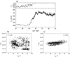 |
Fig. 2. Wind at 1 AU. Panel a: bulk speed, Vsw (lower plot) and v − b correlation coefficient at 1 h scale, Cvb (upper plot); panels b and c: scatter plots of T and θBR for an interval of slow (left) and fast wind (right), respectively, along with the value of the linear correlation coefficient between T and θBR (indicated as C) in the zoomed-in time interval. |
Even with Wind observations we make a comparison between temperature and magnetic field orientation as in the previous section. The results are shown in Fig. 2 with the same format as Fig. 1. Similar to Helios data, the Wind time series is characterized by a transition from a slow to a fast wind stream, allowing us to study different solar wind speed conditions. Panel a shows the solar wind speed profile and the v − b correlation coefficient, Cvb, between the z components given in the GSE (Geocentric Solar Ecliptic) coordinate system. The latter is on average above 0.8 from DoY 30 and 33 keeping its value high within the main portion of the fast stream where velocity fluctuations are larger. On the other hand, the first part of the time interval is characterized by slow speed and low v − b correlation. It is worth noting that not only do slow and fast wind show a different Alfvénic content but Alfvénicy also decreases when moving away from the Sun. The decrease of the correlation coefficient observed in the fast streams at 0.3 AU (Helios) and at 1 AU (Wind) might therefore be explained as an effect of the radial evolution of Alfvénicity in the solar wind and a consequent degradation of the v − b correlation.
Panels b and c show the scatter plots of θBR and T for slow and fast wind, respectively. Visual inspection shows again that T and θBR are better correlated within fast wind than within slow wind. In terms of the T–θBR correlation coefficient, C = 0.50 and −0.11, respectively.
Now that we have verified the behavior of the total temperature with respect to θBR also in Wind data, we move to the anisotropic analysis which allows us to derive the temperature components with respect to the magnetic field direction. We restrict the comparison of θBR with T∥ and T⊥ to the fast wind. Figure 3 shows two panels containing the scatter plots of θBR versus T∥ (upper panel) and T⊥ (lower panel) for the same time interval of fast wind shown in Fig. 2. It can easily be seen that the two temperature components show a different relationship with θBR. Here, T∥ is not correlated with θBR, with a very low correlation coefficient (C = −0.12). On the contrary, T⊥ correlates very well with θBR with a relatively high correlation coefficient of C = 0.57, indicating a positive correlation.
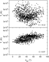 |
Fig. 3. Wind at 1 AU. Upper panel: θBR vs. T∥. Lower panel: θBR vs. T⊥. Results are shown for the interval of fast wind shown in Fig. 2. Each panel also reports the value of the linear correlation coefficient between T components and θBR in that interval. |
It must be noted that the results obtained in such short time intervals are representative of the behavior of the fast and slow wind, respectively. We computed histograms of the correlation coefficient between θBR and the temperature components using a sliding window of 1 h. Fast wind was selected from day 30 to 35 of the year 1995 and slow wind from day 25 to 29 of the same year. Figure 4 shows frequency counts normalized to the total number of cases of the correlation coefficient between θBR and T⊥ (upper panel) and between θBR and T∥ (lower panel). The fast wind interval, characterized by a high degree of v − b correlation, is represented by black circles. On the contrary, the slow wind is characterized by a very low correlation and is represented by empty circles. It must be observed that for slow wind the distribution corresponding to the correlation coefficient for both components is similar with a symmetric and spread distribution that peaks around zero. Fast wind on the contrary shows a different behavior for the two temperature components. Only the perpendicular component shows a skewed distribution shifted towards positive values and peaking around 0.5, while the parallel component is peaked and centered around zero.
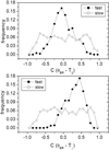 |
Fig. 4. Wind at 1 AU. Frequency counts normalized to the total number of cases of the correlation coefficient between θBR and T∥ (upper panel) and between θBR and T⊥ (lower panel) for fast wind (black circles) and slow wind (empty circles). The time intervals used to compute the histograms are indicated in the text. |
D’Amicis & Bruno (2015) and D’Amicis et al. (2019a) found at 1 AU the presence of slow wind streams characterized by a high Alfvénic content. This result was rather unexpected for several reasons. Firstly, the identification of this Alfvénic slow wind is not limited to case studies only; rather it is found on a statistical basis over a period of 30 months. Moreover, it was found at 1 AU while we would expect a degradation of the Alfvénic correlation due the solar wind expansion. Marsch et al. (1981) was the first to identify Alfvénic slow solar wind at Helios perihelion. D’Amicis & Bruno (2015) then showed that it was characterized by smaller-amplitude fluctuations with respect to fast wind at Helios perihelion. This study was further improved by D’Amicis et al. (2019a) who showed that the Alfvénic slow wind at 1 AU not only has a similar Alfvénic content but also the amplitude of fluctuations is similar to the fast wind streams as also shown by D’Amicis et al. (2019b). To corroborate our findings, we further show in Fig. 5 the results for a representative Alfvénic solar wind stream from day 25 to 35 of the year 2002. The time interval also includes a “typical” slow wind following the Alfvénic slow wind stream. In particular, the left panels show the solar wind speed profile Vsw (lower plot) and v − b correlation coefficient computed at over 1 h scale Cvb (upper plot), between the z components given in the GSE coordinate system. The Alfvénic slow wind stream extends from day 26 to 30. The lower panels show a zoomed-in view of scatter plots of θBR versus T∥ (upper panel) and θBR versus T⊥ (lower panel). Also in this case, similar to the fast wind case, there is a positive correlation between θBR and the perpendicular temperature component but no such correlation is seen with the parallel component. The linear correlation coefficient between T components and θBR in the two cases is 0.05 and 0.58, respectively.
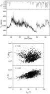 |
Fig. 5. Wind at 1 AU. Upper panels: bulk speed Vsw (lower plot) and correlation coefficient at 1 h scale Cvb (upper plot). The dashed red box marks the main portion of the Alfvénic slow wind stream. Lower panels: zoom of the time interval showing the scatter plots of θBR vs. T∥ (upper panel) and θBR vs. T⊥ (lower panel). The panels also show the value of the linear correlation coefficient between T components and θBR. |
To summarize, both Helios 2 at 0.3 AU and Wind observations at 1 AU have shown a positive correlation existing between the proton temperature and the magnetic field orientation. This behavior has to be intended as qualitative rather than quantitative. However, the correlation found in Helios observations can be explained as in Gogoberidze et al. (2018), considering that we are dealing with the radial component of temperature derived from 1D VDF which by definition is related to θBR. Nevertheless, in Wind measurements at 1 AU, temperature components are derived from 3D VDF and the correlation between T and θBR found at the shortest available timescale and clearly appearing only within the Alfvénic winds (both fast and slow) can be interpreted as due to a physical mechanism. In particular, the correlation observed between the perpendicular component and the magnetic field direction, and a lack of correlation with the parallel component, would suggest a role of the cyclotron resonant mechanism.
3. Numerical simulations – evaluating instrumental effects
We now estimate whether or not a long-lasting particle velocity distribution measurement like the one performed by Helios/I1a has an impact on the proton temperature anisotropy value. Our goal is to numerically simulate the typical sampling of the VDF operated by a quadrispherical electrostatic analyzer in order to estimate any possible artificial contribution to the temperature anisotropy and perform a comparison with observations.
Verscharen & Marsch (2011) addressed the question of “apparent” temperature anisotropies due to wave activity in solar wind. As a matter of fact, a low plasma β bi-Maxwellian VDF with equal parallel and perpendicular temperature with respect to the ambient magnetic field is shaped by the presence of a large-amplitude Alfven-cyclotron wave. In this case, the VDF displays a sloshing motion perpendicular to B, which when averaged by the process of measurement, leads to a greater perpendicular temperature. However, Nicolaou et al. (2019) showed that typical fluctuations due to solar wind turbulence (e.g., Alfvénics fluctuations and slow modes) have only minor effects on moment computation and those effects decrease with decreasing acquisition time. The numerical study has been performed taking into account the fact that the VDF sampled by an electrostatic analyzer can be obtained from the particle counts considering that

where dN is the number of counts with velocity vector v which pass in a time dt through the aperture with area S with direction along the inward normal, f(v) is the VDF and G(v) is the response function, that is the probability that a particle with velocity v incident on the sensor will be counted. G(v) is different from zero in a limited region of space, namely the field of view (FOV) of the sensor.
Considering the instrumental elementary acceptance volume ΔvΔΘΔΦ and time of acceptance Tacc, Eq. (2) becomes
![$$ \begin{aligned} N_{{ v}\Theta \Phi } = f_{{ v}\Theta \Phi }[G]{ v}^4 T_{\rm acc}, \end{aligned} $$](/articles/aa/full_html/2019/12/aa36728-19/aa36728-19-eq6.gif)
where G is the geometrical factor, which relates the number of particles detected to the flux incident on the instrument, and is evaluated through a calibration procedure in the laboratory. Equation (3) can be easily inverted to compute the 3D VDF once the number of particles in each pixel is known. The moments of the VDF of a given particle species are defined as
where vn is an n-fold dyadic product. The zero-order moment is the number density, N. The bulk speed U is derived from the first-order moment which is the number flux density vector, NU. The second- and third-order moments are the momentum flux density tensor, Π, and the energy flux density vector, Q, from which the pressure tensor (and then temperature) and the heat flux, respectively, can be derived after moving in the plasma frame (v-U).
When calculating moments, the VDF is given in terms of count rates by Eq. (3), with integrals replaced by sums referred to the field of view and energy steps of the sensor. A question that is often debated is whether or not the sampling time of the VDF, which can be long compared to the typical times of the wave–particle interaction processes, may alter the VDF while it is being measured, resulting eventually in distorted moments. The need for long sampling times is due essentially to the low density of particles in solar wind. The geometrical factor can also be a limit, since the sensor capabilities represent a trade-off between the measurement requirements and resources available, in terms of mass, power, and electronics.
In order to understand whether or not the acquisition of the proton VDF (and the following definition of moments) onboard the s/c can be affected by the presence of Alfvén waves, we performed a numerical simulation of this measurement process by means of a sensor with technical characteristics similar to that of the I1a sensor for positive ions flown onboard Helios s/c. To this aim, a top-hat electrostatic analyzer was simulated (Carlson et al. 1983) allowing selection of charged particles according to specific energy and angular criteria. The I1a sensor has 32 energy steps Ei, ranging from 155 to 15320 eV, nine polar angles Θj, from −22.5° to 22.5°, and an azimuth of 87° divided into 16 anodes Φk. The energy steps are contiguous and logarithmically spaced. A different energy interval is acquired for each s/c rotation, which in our simulation lasts 1 s, meaning that the acquisition of the whole VDF takes 32 s. In any case, considering that the solar wind proton distribution is usually very focused and occupies a small portion of the FoV, the real acquisition time is roughly one-third of this.
The usual way to perform computer simulations for moment computation is to consider a bi-Maxwellian VDF with a given number density, bulk velocity, and temperature. This is converted into particles counts using Eq. (3), detected by a sensor with the specified response characteristics. Particles are then added with Poissonian noise and moment integration is carried out. For the present case, we carry out a simulation in which the VDF is dynamically modified during the acquisition process according to wave activity and compare the moments thus obtained to those found in the unperturbed case. We consider here only perturbation to the bulk velocity induced by Alfvén waves propagating parallel to the ambient magnetic field. The acquisition time interval of the VDF is partitioned in subintervals of 1 s each s/c rotation in which a different energy step and/or direction is sampled. For each subinterval the bulk velocity is given by
where ti represents the elementary acquisition time, that is the acquisition time of ith energy step, and  , and
, and  are the averaged velocity, mass density, and magnetic field during the current measure. Thus, for each ti a new VDF is generated with the same given temperature and density, but different velocity. The overall result is that the sensor “sees” a VDF subject to a rigid shift during the measure, but no deformation of the VDF takes place.
The initial condition is represented by a solar wind with a purely radial bulk velocity of 700 km s−1 and a number density of 30 cm−3. Initial temperatures are taken equal to 50 eV (5.8 × 10⁵ K) both parallel and perpendicular to the magnetic field. We use magnetic field data measured from Helios at 1 AU at 4 Hz and then averaged at 1 Hz, for a time interval of around 13.8 h and a total of 1552 mock-up distributions.
For a single acquisition of a VDF the angle θBR during the measurement time can be quantified as
where  and
and  are the unit vectors associated to magnetic field and radial direction, respectively and N is the number of energy steps. Figure 6 shows the scatter plots of θBR vs. T∥ (upper panel) and θBR vs. T⊥ (lower panel) as derived by numerical simulations. In both cases, the two quantities are spread in the scatter plots and appear clearly uncorrelated. Specifically, the correlation coefficients between T components and θBR are 0.07 and 0.1 for T∥ and T⊥, respectively, thus proving that the acquisition of an electrostatic analyzer in the presence of Alfvénic fluctuations does not introduce any artificial anisotropy.
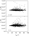 |
Fig. 6. Scatter plots of θBR vs. T∥ (upper panel) and θBR vs. T⊥ (lower panel) as derived by numerical simulations reproducing the acquisition of an electrostatic analyzer. Correlation coefficients between T components and θBR are indicated in the two panels. |
It must be noted that this result applies for an electrostatic analyzer like the I1a instrument onboard Helios sampling the 3D VDF in about 32 s. Thus, it is still valid for the 3DP instrument onboard Wind which has a faster acquisition time.
4. Summary and conclusions
In the present paper we analyze and compare Helios observations at 0.3 AU with Wind observations at 1 AU. The motivation for our work comes from the fact that if Alfvénic fluctuations have a role in plasma heating, we should be able to find a correlation between the magnetic field noncompressive fluctuations and the proton temperature level simply from the raw plasma and magnetic field data, as described in Sect. 1. We then search in both databases for a clear relationship between field orientation and plasma temperature, using the angle the magnetic field forms with a fixed direction, such as for example the radial direction.
We found a positive correlation between temperature and magnetic field orientation, studied by means of θBR, on a scale of 40.5 s for Helios data at 0.3 AU within the fast and highly Alfvénic wind and no correlation within slow wind. However, the correlation found in Helios observations can be explained as in Kasper et al. (2002) and Gogoberidze et al. (2018). Furthermore, the available Helios temperature is the radial component derived from 1D VDF which by definition is related to θBR. This is true for an anisotropic VDF in which pseudo-thermal fluctuations (see Gogoberidze et al. 2018) responsible for the correlation are driven by large-amplitude Alfvénic fluctuations.
Successively, we used Wind data at 24 s resolution. In this case, temperature components are derived from canonical moment computation and the correlation between T and θBR, found at the shortest available timescale and clearly appearing only within the Alfvénic winds (both fast and slow), could be attributed to a physical mechanism. Moreover, as expected, the slow and non Alfvénic wind confirmed the absence of such correlations. Finally, the temperature anisotropy data from Wind gave us the possibility to show that the correlation between magnetic field and total temperature is due only to the perpendicular component of the proton temperature rather than to the parallel component. This might be interpreted as an ion cyclotron resonant mechanism as has been reported several times in the literature (e.g., see reviews by Tu & Marsch 1995; Hollweg & Isenberg 2002). In particular, the large perpendicular temperature anisotropy shown in Helios observations, together with the regulation of the anisotropy by pitch angle diffusion of solar wind protons in resonance with cyclotron waves (Tu & Marsch 2002), represent clear evidence.
Our interpretation is in agreement with the results by Bruno & Telloni (2015) and Telloni & Bruno (2016). Those authors identified signatures of Ion-Cyclotron Waves (ICWs) within the main portion of fast streams. The presence of ICWs might be related to fluid-scale Alfvénic fluctuations, this time characterizing intervals which would experience cyclotron resonance with protons (Bruno & Trenchi 2014) causing an enhanced temperature anisotropy. It must be stressed however that although this study provides a possible explanation of our observations in terms of the ion-cyclotron mechanism, it does not exclude the contribution of other possible kinetic nonresonant mechanisms.
There are also other mechanisms which might play a role in heating the protons, as reported in the introduction, and there is a lack of convergence within the community towards the identification of the primary physical mechanism at the basis of heating and acceleration of the solar wind plasma. This is mainly due to the fact that we still lack sufficiently fast sampling of the VDFs of protons, electrons, and minor ions. In particular, we lack this kind of measurement close enough to the Sun where wave-particle coupling is stronger. Sufficiently fast near-Sun plasma and field measurements are therefore of key importance in determining which mechanism plays the major role and the next two heliospheric missions Parker Solar Probe and Solar Orbiter will fulfill this requirement.
Finally, we simulated the sampling procedure of the proton VDF followed by an electrostatic analyzer in search of possible instrumental effects. We proved that the correlation between magnetic field orientation and proton temperature is not caused by a smearing of the distribution due to a long-lasting VDF measurement during which Alfvénic fluctuations would cause an incorrect evaluation of the perpendicular temperature component in agreement with Nicolaou et al. (2019). In addition, our simulations also excluded the introduction of an artificial temperature anisotropy of instrumental origin.
We conclude that while the relationship between θBR and T in the original Helios plasma data is dominated by effects produced by a noncanonical plasma data reduction, results from Wind would suggest that this effect is genuine since T is derived from a 3D VDF. In the Helios case, the functional relation in Eq. (1) implies an artificial correlation between θBR and TR. In the Wind case, the qualitative dependence of the perpendicular temperature on θBR would suggest an active role of the proton cyclotron resonance mechanism at the basis of the observed temperature anisotropy. However, we would also expect a correlation between θBR and T⊥ in the reprocessed Helios data, but this is not the case. The fact that we find this effect in Wind, and in particular in T⊥, might be ascribed to two different situations: one where the effect is genuine and might be associated to the presence of Alfvénic fluctuations experiencing ion-cyclotron resonance with protons; and another where the effect, for some reason, is artificial and temperature anisotropy of 3DP Wind data is not reliable. However, we cannot give a definitive answer. The different results of reprocessed Helios and Wind data therefore require further investigation with particular reference to the way moments (in particular temperature components) are derived from 3D VDFs in order to verify whether or not the fitting procedure could affect the moment computation itself. This is a very important issue in view of the interpretation of plasma data coming from the Parker Solar Probe and from Solar Orbiter.
Acknowledgments
The authors are grateful to the following people and organizations for data provision: R. Schwenn (Max Planck Institute) for Helios/E1, F. Neubauer (University of Cologne) for Helios/E3, R. Lin (UC Berkeley) for Wind/3DP, R. P. Lepping (NASA/GSFC) for Wind/MFI data. All these data are available on the NASA-CDAWeb website: https://cdaweb.sci.gsfc.nasa.gov/index.html. The authors also aknowledge the use of the reprocessed Helios data available on http://helios-data.ssl.berkeley.edu/data/. Results from the simulation presented in this paper are directly available from the authors. The authors thank the reviewer for helping in improving this paper. This research was partially supported by the Agenzia Spaziale Italiana under contract 2018-30-HH.O.
References
- Bourouaine, S., & Chandran, B. D. G. 2013, ApJ, 774, 96 [NASA ADS] [CrossRef] [Google Scholar]
- Bourouaine, S., Marsch, E., & Neubauer, F. M. 2010, Geophys. Res. Lett., 37, 14104 [NASA ADS] [CrossRef] [Google Scholar]
- Bruno, R., Bavassano, B., & Villante, U. 1985, J. Geophys. Res., 90, 4373 [NASA ADS] [CrossRef] [Google Scholar]
- Bruno, R., Carbone, V., Primavera, L., et al. 2004, Ann. Geophys., 22, 3751 [Google Scholar]
- Bruno, R., Bavassano, B., D’Amicis, R., et al. 2006, AGU Fall Meeting Abstracts 2006, SH14A [Google Scholar]
- Bruno, R., & Carbone, V. 2013, Liv. Rev. Sol. Phys., 10, 2 [Google Scholar]
- Bruno, R., & Telloni, D. 2015, ApJ, 811, L17 [Google Scholar]
- Bruno, R., & Trenchi, L. 2014, ApJ, 787, L24 [NASA ADS] [CrossRef] [Google Scholar]
- Bruno, R., Trenchi, L., & Telloni, D. 2014, ApJ, 793, L15 [NASA ADS] [CrossRef] [Google Scholar]
- Carlson, C. W., Curtis, D. W., Paschmann, G., & Michael, W. 1983, Adv. Space Res., 2, 67 [Google Scholar]
- Chandran, B. D. G., Li, B., Rogers, B. N., et al. 2010, ApJ, 720, 503 [NASA ADS] [CrossRef] [Google Scholar]
- D’Amicis, R., & Bruno, R. 2015, ApJ, 805, 84 [NASA ADS] [CrossRef] [Google Scholar]
- D’Amicis, R., Matteini, L., & Bruno, R. 2019a, MNRAS, 483, 4665 [NASA ADS] [Google Scholar]
- D’Amicis, R., Matteini, L., & Bruno, R. 2019b, Sol. Phys., submitted [Google Scholar]
- Denskat, K. U., Beinroth, H. J., & Neubauer, F. M. 1983, J. Geophys. – Z. Geophys., 54, 60 [Google Scholar]
- Dong, C. 2014, Phys. Plasmas, 21, 022302 [NASA ADS] [CrossRef] [Google Scholar]
- Dmitruk, P., Matthaeus, W. H., & Seenu, N. 2004, ApJ, 617, 667 [NASA ADS] [CrossRef] [Google Scholar]
- Gogoberidze, G., Voitenko, Y. M., & Machabeli, G. 2018, MNRAS, 480, 1864 [NASA ADS] [CrossRef] [Google Scholar]
- Hollweg, J. V., & Isenberg, P. A. 2002, J. Geophys. Res., 107, 1147 [CrossRef] [Google Scholar]
- Kasper, J. C., Lazarus, A. J., & Gary, S. P. 2002, Geophys. Res. Lett., 29, 1839 [NASA ADS] [CrossRef] [Google Scholar]
- Leamon, R. J., Smith, C. W., Ness, N. F., et al. 1998, J. Geophys. Res., 103, 4775 [NASA ADS] [CrossRef] [Google Scholar]
- Lepping, R. P., Acuña, M. H., Burlaga, L. F., et al. 1995, Space Sci. Rev., 71, 207 [NASA ADS] [CrossRef] [Google Scholar]
- Lin, R. P., Anderson, K. A., Ashford, S., et al. 1995, Space Sci. Rev., 71, 125 [NASA ADS] [CrossRef] [Google Scholar]
- Mariani, F., Ness, N. F., Burlaga, L. F., et al. 1978, J. Geophys. Res., 83, 5161 [NASA ADS] [CrossRef] [Google Scholar]
- Marsch, E., Rosenbauer, H., Schwenn, R., et al. 1981, J. Geophys. Res., 86, 9199 [NASA ADS] [CrossRef] [Google Scholar]
- Marsch, E., Schwenn, R., Rosenbauer, H., et al. 1982, J. Geophys. Res., 87, 52 [NASA ADS] [CrossRef] [Google Scholar]
- Marsch, E. 2006, Liv. Rev. Sol. Phys., 3, 1 [Google Scholar]
- Marsch, E. 2012, Space Sci. Rev., 172, 23 [NASA ADS] [CrossRef] [Google Scholar]
- Nariyuki, Y., Hada, T., & Tsubouchi, K. 2010, Phys. Plasmas, 17, 072301 [NASA ADS] [CrossRef] [Google Scholar]
- Nicolaou, G., Verscharen, D., Wicks, R. T., & Owen, J. 2019, ApJ, 886, 101 [NASA ADS] [CrossRef] [Google Scholar]
- Osman, K. T., Matthaeus, W. H., Greco, A., & Servidio, S. 2011, ApJ, 727, L11 [NASA ADS] [CrossRef] [Google Scholar]
- Perrone, D., D’Amicis, R., De Marco, R., et al. 2019, A&A, submitted [Google Scholar]
- Rosenbauer, H., Schwenn, R., Marsch, E., et al. 1977, J. Geophys., 42, 561 [Google Scholar]
- Scearce, C., et al. 1975, NASA/GSFC Tech. Rep. X-692-75-112 [Google Scholar]
- Stansby, D., Salem, C., Matteini, L., & Horbury, T. 2018, Sol. Phys., 293, 155 [NASA ADS] [CrossRef] [Google Scholar]
- Stansby, D., Matteini, L., Horbury, T. S., et al. 2019, MNRAS, submitted [Google Scholar]
- Telloni, D., & Bruno, R. 2016, MNRAS, 463, L79 [NASA ADS] [CrossRef] [Google Scholar]
- Tu, C.-Y., & Marsch, E. 1995, Space Sci. Rev., 73, 1 [Google Scholar]
- Tu, C.-Y., & Marsch, E. 2002, J. Geophys. Res., 107, 1249 [CrossRef] [Google Scholar]
- Tu, C.-Y., Pu, Z.-Y., & Wei, F.-S. 1984, J. Geophys. Res., 89, 9695 [NASA ADS] [CrossRef] [Google Scholar]
- Vasquez, B. J., & Hollweg, J. V. 2001, J. Geophys. Res., 106, 5661 [NASA ADS] [CrossRef] [Google Scholar]
- Verscharen, D., & Marsch, E. 2011, Ann. Geophys., 29, 909 [NASA ADS] [CrossRef] [Google Scholar]
- Voitenko, Y., & Goossens, M. 2004, Nonlinear Proc. Geophys., 11, 535 [NASA ADS] [CrossRef] [Google Scholar]
- Wang, C. B., Wu, C. S., & Yoon, P. H. 2006, Phys. Rev. Lett., 96, 125001 [NASA ADS] [CrossRef] [Google Scholar]
- Wu, C. S., & Yoon, P. H. 2007, Phys. Rev. Lett., 99, 075001 [NASA ADS] [CrossRef] [Google Scholar]
- Zhang, T.-X., Wang, J.-X., & Xiao, C.-J. 2005, Chin. J. Astron. Astrophys., 5, 285 [NASA ADS] [CrossRef] [Google Scholar]
All Figures
|
Fig. 1. Helios 2 at 0.3 AU. Panel a: bulk speed, Vsw (lower plot), and the v − b correlation coefficient at 1 h scale, Cvb (upper plot). Panels b and c: scatter plots of TR (as derived with Eq. (1)) and θBR for an interval of slow wind (left) and fast wind (right), respectively, using data from NASA website CDAWeb (https://cdaweb.sci.gsfc.nasa.gov), indicated as original. Panels d and e: analogous to panels b and c, respectively, for data from the Space Sciences Laboratory University of California (Berkeley) dataset (http://helios-data.ssl.berkeley.edu/data/), indicated as reprocessed. We show also the scatter plots of the total temperature T vs. θBR referring to reprocessed data in panels f and g. Panels b–g: we report also the value of the linear correlation coefficient, C, between TR (or T) and θBR, in the zoomed time intervals. |
| In the text | |
|
Fig. 2. Wind at 1 AU. Panel a: bulk speed, Vsw (lower plot) and v − b correlation coefficient at 1 h scale, Cvb (upper plot); panels b and c: scatter plots of T and θBR for an interval of slow (left) and fast wind (right), respectively, along with the value of the linear correlation coefficient between T and θBR (indicated as C) in the zoomed-in time interval. |
| In the text | |
|
Fig. 3. Wind at 1 AU. Upper panel: θBR vs. T∥. Lower panel: θBR vs. T⊥. Results are shown for the interval of fast wind shown in Fig. 2. Each panel also reports the value of the linear correlation coefficient between T components and θBR in that interval. |
| In the text | |
|
Fig. 4. Wind at 1 AU. Frequency counts normalized to the total number of cases of the correlation coefficient between θBR and T∥ (upper panel) and between θBR and T⊥ (lower panel) for fast wind (black circles) and slow wind (empty circles). The time intervals used to compute the histograms are indicated in the text. |
| In the text | |
|
Fig. 5. Wind at 1 AU. Upper panels: bulk speed Vsw (lower plot) and correlation coefficient at 1 h scale Cvb (upper plot). The dashed red box marks the main portion of the Alfvénic slow wind stream. Lower panels: zoom of the time interval showing the scatter plots of θBR vs. T∥ (upper panel) and θBR vs. T⊥ (lower panel). The panels also show the value of the linear correlation coefficient between T components and θBR. |
| In the text | |
|
Fig. 6. Scatter plots of θBR vs. T∥ (upper panel) and θBR vs. T⊥ (lower panel) as derived by numerical simulations reproducing the acquisition of an electrostatic analyzer. Correlation coefficients between T components and θBR are indicated in the two panels. |
| In the text | |
Current usage metrics show cumulative count of Article Views (full-text article views including HTML views, PDF and ePub downloads, according to the available data) and Abstracts Views on Vision4Press platform.
Data correspond to usage on the plateform after 2015. The current usage metrics is available 48-96 hours after online publication and is updated daily on week days.
Initial download of the metrics may take a while.