| Issue |
A&A
Volume 632, December 2019
|
|
|---|---|---|
| Article Number | A23 | |
| Number of page(s) | 11 | |
| Section | Stellar atmospheres | |
| DOI | https://doi.org/10.1051/0004-6361/201936307 | |
| Published online | 22 November 2019 | |
Surprises in the simultaneous X-ray and optical monitoring of π Aquarii★
1
Groupe d’Astrophysique des Hautes Energies, STAR, Université de Liège, Quartier Agora (B5c, Institut d’Astrophysique et de Géophysique),
Allée du 6 Août 19c, 4000 Sart Tilman, Liège, Belgium
e-mail: This email address is being protected from spambots. You need JavaScript enabled to view it.
2
National Optical Astronomy Observatory,
950 N Cherry Ave, Tucson, AZ 85721, USA
Received:
13
July
2019
Accepted:
17
October
2019
Abstract
To help constrain the origin of the peculiar X-ray emission of γ Cas stars, we conducted a simultaneous optical and X-ray monitoring of π Aqr in 2018. At that time, the star appeared optically bright and active, with a very strong Hα emission. Our monitoring covers three 84 d orbital cycles, allowing us to probe phase-locked variations as well as longer-term changes. In the new optical data, the radial velocity variations seem to span a smaller range than previously reported, which might indicate possible biases. The X-ray emission is variable, but without any obvious correlation with orbital phase or Hα line strength. Furthermore, the average X-ray flux and the relative range of flux variations are similar to those recorded in previous data, although the latter data were taken when the star was less bright and its disk had nearly entirely disappeared. Only the local absorption component in the X-ray spectrum appears to have strengthened in the new data. This absence of large changes in X-ray properties despite dramatic disk changes appears at odds with previous observations of other γ Cas stars. It also constrains scenarios proposed to explain the γ Cas phenomenon.
Key words: stars: early-type / stars: emission-line, Be / stars: massive / X-rays: stars / supernovae: general / stars: individual: π Aqr
Based on spectra obtained with the TIGRE telescope, located at La Luz observatory, Mexico (TIGRE is a collaboration of the Hamburger Sternwarte, the Universities of Hamburg, Guanajuato, and Liège), as well as data collected with the Neil Gehrels Swift Observatory.
F.R.S.-FNRS Senior Research Associate.
© ESO 2019
1 Introduction
Massive stars have decades ago been found to emit X-rays. This high-energy emission may be linked to accretion onto a compact object either from their stellar wind or through Roche-lobe overflow, when they are part of high-mass X-ray binaries. The ensuing X-ray emission is hard and extremely intense. On the other hand, shocks within the stellar wind or between two stellar winds in massive binaries also lead to the emission of X-rays, but this thermal emission is much softer (kT ~ 0.6−2 keV) and dimmer (log[LX∕LBOL] ~ −7 to –6).
In between these two extremes are γ Cas analogs, named after their prototype, the central star of the Cassiopeia constellation. These stars exhibit a thermal spectrum with a high plasma temperature (kT = 5–15 keV) and a fluorescent iron line at 6.4 keV in the iron complex. Their (variable) brightness is intermediate between “normal” OB-stars and X-ray binaries (log[LX∕LBOL] between –6 and –4). Currently, about 20 such objects are known (see Smith et al. 2016; Nazé & Motch 2018).
The origin of the peculiar X-ray emission of γ Cas stars remains debated. Two main classes of scenarios have been proposed. On the one hand, X-rays could be emitted by an accreting white dwarf (Murakami et al. 1986) or by an accreting neutron star in the propeller regime (Postnov et al. 2017). On the other hand, X-rays could be emitted by star-disk interactions occurring through localized magnetic fields in the disk, which could be generated by disk instabilities (Smith et al. 1998; Smith & Robinson 1999), and in the star, possibly arising from a subsurface equatorial convective zone (Cantiello et al. 2009; Motch et al. 2015). In both cases, changes in the disk are expected to eventually affect the X-ray emission, possibly after some delay, depending on the model under consideration.
Monitoring therefore is an essential tool for understanding the γ Cas phenomenon, and we therefore decided to undertake a simultaneous X-ray and optical monitoring of π Aqr in 2018. This recently discovered (Nazé et al. 2017) example of a γ Cas star is a known binary with a period of 84.1 d (Bjorkman et al. 2002, see Table 1). If the peculiar X-ray emission of γ Cas stars is linked to accretion, the low-mass companion detected by Bjorkman et al. (2002) would have to be the compact accretor (although these authors favored a non-degenerate nature). There is no room in the system for a third object to orbit close to (and to accrete from) the disk in a stable way.
Our monitoring fully covered three orbital cycles of π Aqr in order to ascertain the presence of phase-locked changes of the X-ray emission. These variations could occur because the orbital inclination of the system is rather high (70°) and the companion was known to affect the disk geometry (Zharikov et al. 2013). Comparing the new data to older X-ray detections also allows us to study the longer-term variations, if any. This article reports the results of this variability study. Aftera brief summary of the observations and their reduction (Sect. 2), the behavior of π Aqr in the optical and X-ray domains is examined (Sects. 3 and 4, respectively) before we draw a short conclusion (Sect. 5).
Properties of π Aqr as reported by Bjorkman et al. (2002).
2 Observations and data reduction
2.1 Optical spectroscopy
We monitored three orbits of π Aqr in April–December 2018 with the fully robotic 1.2 m TIGRE telescope (Schmitt et al. 2014) installed at La Luz Observatory near Guanajuato (Mexico). The telescope is equipped with the refurbished HEROS echelle spectrograph covering the wavelength domain from 3800 to 8800 Å, with a small 100 Å wide gap near 5800 Å. The resolving power is about 20 000. The data reduction was performed with the dedicated TIGRE/HEROS reduction pipeline (Mittag et al. 2011). Absorption by telluric lines was corrected within IRAF using the template of Hinkle et al. (2000) around the He I λ 5876 Å, Hα, O, and Fe lines in 7400–7850 Å, as well as the Paschen lines at 8350–8800 Å. As a last step, the high-resolution spectra were normalized over limited wavelength windows using splines of low order. The journal of the observations is provided in Table 2.
2.2 X-ray data
Simultaneously with the optical campaign, π Aqr was observed 35 times by the Neil Gehrels Swift Observatory in April–December 2018. One of these observations (ObsID = 00010659015) was stopped before pointing had settled, the source appeared on the edge of the detector in another observation (ObsID = 00010659030), and it fell onto bad pixels in a third observation (ObsID = 00010659037), making these three observations unusable. Two additional observations (ObsID = 00010659012 and 21) lasted less than 200 s, hence were too short to provide a detectable signal for the target. Table 3 provides the journal of the remaining 30 observations, which have a typical duration of 1 ks.
Because π Aqr is a bright source at optical and UV wavelengths, the XRT data were taken in Windowed Timing mode to avoid optical loading. To eliminate any remaining contamination, we used only the best-quality (grade = 0) events. The UK online tool1 was used to extract spectra for each observation as well as corrected (full point spread function, PSF) count rates in the 0.5–10. keV energy band. No reliable count rates could be produced online for three observations (ObsID = 00010659008, 16, and 39), however, hence they are missing from Table 3.
In parallel, we also processed the data locally using the XRT pipeline of HEASOFT v6.22.1 with calibrations v20170501. The source spectra were extracted within a circular aperture centered on the Simbad coordinates of the source. Following recommendations of the XRT team, a small radius of 20 px was used to minimize the background contribution; in a few cases, when the source appeared closer to the edge, it was even further reduced to 10 px. For the background estimate, we again followed theXRT team recommendations and used the surrounding annular region with radii 70 and 130 px. Because Windowed Timing data from a single snapshot are compressed in a single row, the spectral scaling parameter (BACKSCAL keyword in header) had to be modified from the areas of the circular regions to their diameters2, that is, to a value of 40 (or 20) for the source and 59 for the background. The adequate RMF matrix from the calibration database was used, and specific ARF response matrices were calculated for each dataset using xrtmkarf, considering the associated exposure map. Both local and online spectra were finally binned using grppha to reach at least 10 cts per bin.
Journal of the TIGRE observations of π Aqr.
3 Optical and near-infrared lines of π Aqr
The optical and near-infrared (NIR) spectrum of π Aqr from our data is shown in Fig. 1. It is dominated by strong emissions of hydrogen (Balmer Hα and Hβ, as well as Paschen lines). Additional emissions, linked to Fe II but also to O I and O III, are detected. Absorption lines include He I lines and several interstellar lines (Na I, Ca II, and diffuse interstellar bands; DIBs). Some lines, such as other Balmer lines and He I λλ4471, 5876 Å, display a mixed absorption and emission content, however.
To characterize the lines, we calculated moments after subtracting 1 from the normalized (see Sect. 2.1) spectra: M0 = ∑ (Fi − 1), M1 = ∑ (Fi − 1) × vi∕∑ (Fi − 1), and  where vi is the radial velocity and Fi the normalized flux. They provide the equivalent width3 EW, the line centroid, and the square of the line width, respectively. For each line, we limited the calculation to a wavelength interval covering most of the profile while avoiding nearby lines or the continuum regions. While the errors on moments can be calculated using error propagation, the interstellar lines provide a check and typical values. The average moments of the interstellar Na I λ 5895.924 Å line, estimated between –25 and 5 km s−1, are M0 = 0.214 ± 0.008Å, M1 = −9.2 ±0.5 km s−1, and a width
  km s−1 (the errors here correspond to dispersions around the means). In the same velocity intervals, the values for the interstellar Ca II λ 3933.663 Å and Ca II λ 3968.468 Å are M0 = 0.095 ± 0.007Å, M1 = −10.7 ± 0.4 km s−1,
  0.4 km s−1, and M0 = 0.109 ± 0.008Å, M1 = −10.3 ± 0.5 km s−1,
  km s−1, respectively. The <1 km s−1 uncertainty in velocity is typical of the wavelength accuracy of TIGRE data (M. Mittag, priv. comm.). Finally, the values for the DIB at 6613.62 Å, estimated between –50 and 60 km s−1, are M0 = 0.032 ± 0.005Å, M1 = −1.7 ± 2.5 km s−1, with a width
  km s−1; the uncertainties are larger because the line is much weaker and broader.
Throughout our campaign, the Hα emission strengthened, with EWs evolving from –22 to –25 Å (Fig. 2, Table 2). Other hydrogen lines follow that behavior (i.e., more emission or less absorption in more recent times), except for H9, whose absorption increased, and the blends H I λ8437 Å + O Iλ8446 Å and H I λ8502 Å, whose emissions decreased. He I and metallic lines displayed small changes in line strength but without a clear trend with time, except for He I λ3819,4471 Å and Mg II λ4481 Å, whose absorptions increased.
Finally, we note that the amplitude of the violet peak with respect to the red peak evolves with time, following a similar behavior in Hα and Hβ emissions (Fig. 3). However, there is no clear correlation with orbital phase, as has been reported for recent years by Nazé et al. (2019). Moreover, π Aqr seems to have recently brightened in the optical domain (V band) as itsemission strengthened (Fig. 4). A similar correlation was detected for γ Cas (Smith et al. 2012), but the opposite trend was found for HD 45314 (Rauw et al. 2018). These positive and negative correlations have been theoretically explained by Sigut & Patel (2013) by way of differences in disk inclination (higher inclinations leading to inverse correlations) but also in disk scale heights.
X-ray properties of π Aqr derived from Swift observations.
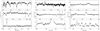 |
Fig. 1 Spectrum of π Aqr taken by TIGRE on 10 July 2018, after correction of the telluric lines. |
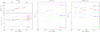 |
Fig. 2 Evolution with time of zeroth-order moments (EWs) for hydrogen, He I, and metallic lines. In these panels, higher emissions (absorptions) are toward the top (bottom). For Hα, the values derived from amateur data reported by Nazé et al. (2019) are also shown as small red crosses. |
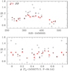 |
Fig. 3 Evolution with time or phase of the V∕R for the Hα and Hβ lines. |
3.1 Radial velocities
In addition to the first-order moment of the full profile, we evaluated the radial velocity (RV) of Hα using two other techniques focusing on the line wings that were previously applied to the case of γ Cas. The first technique compares the line profile and its mirror (after reversing velocities) for different shifts, searching for the least difference between them (Nemravová et al. 2012, and references therein). Only the wings between approximately 20 and 60% of the maximum amplitude were considered in this calculation for γ Cas. This corresponds to normalized fluxes of 1.4 and 2.2 for π Aqr because the profile peaks around a normalized flux of 3 in 2018. Shifts from –50 to +50 km s−1 were examined, with steps of 0.5 km s−1. A parabolic fitting of the χ2 values was then made to find the final best shift, which corresponds to −RV. The second technique correlates the line profile to the two-Gaussians function ![Mathematical equation: $G(v)\,{=}\,\textrm{exp}[-(v-a)^2/2\sigma^2]-\textrm{exp}[-(v+a)^2/2\sigma^2]$](/articles/aa/full_html/2019/12/aa36307-19/aa36307-19-eq6.png) (Smith et al. 2012, based on Shafter et al. 1986). The RV is then found when the correlation reaches zero. The Gaussian center a and width σ were chosen to be 245 and 20 km s−1, respectively, to allow us to derive the velocity near the half-maximum of the line (i.e., it is a bisector value).
(Smith et al. 2012, based on Shafter et al. 1986). The RV is then found when the correlation reaches zero. The Gaussian center a and width σ were chosen to be 245 and 20 km s−1, respectively, to allow us to derive the velocity near the half-maximum of the line (i.e., it is a bisector value).
The left panel of Fig. 5 compares the velocities derived for the Hα line by these three different techniques (see Table 2 for values), revealing a good agreement between them. The dispersion for first-order moments appears larger, but this is to be expected because they probe the entire line profile, including the most strongly varying central regions. The right panel of the same figure displays these velocities folded with the mean ephemeris of Bjorkman et al. (2002). It also compares them to the orbital solution of Bjorkman et al. (2002) for the primary star. We recall that this solution was derived by using the mirror method on the absorption component (photosphere of the primary) because the disk had nearly completely disappeared at the time of their observations, while our values correspond to the velocities of the emission component (disk of the primary) because the disk now strongly dominates the Hα line.
Two conclusions can be drawn. First, there seems to be no phase shift, showing that the Bjorkman ephemeris remains accurate to this day. Second, a mismatch in amplitude is clearly detected: Bjorkman et al. (2002) inferred a semi-amplitude K1 of 16.7 km s−1 for the Hα absorption observed at that time, while the semi-amplitude recorded for the Hα emission in 2018 only amounts to half this value. At first, this decrease might be attributed to the blend with the companion line and/or the imperfect symmetry of the disk. Because the disk appears slightly brighter on the companion side (see Sect. 3.2 and Nazé et al. 2019), the derived velocities could be biased toward the companion velocity. A blend would have a similar effect. This would imply that velocities derived from the Be disk emissions may not be fully representative of the Be star’s true velocity, although emissions such as Hα are commonly used to this aim (see, e.g., Nemravová et al. 2012 or Smith et al. 2012 for γ Cas).
However, the three methods for deriving Hα velocities sample very different regions of the disk but yield very similar results. The moment method uses the full line profile, including any potential (direct or indirect) signature of the companion. The two-Gaussian correlation method only examines the line profile in a very small interval near its half-maximum (which occurs near ± 245 km s−1), and the mirror method only examines wings, approximately in the intervals between ± 375 and ± 210 km s−1. These two methods therefore probe regions that are not affected by the companion line because its velocity lies between –100 and 100 km s−1 (Bjorkman et al. 2002), but they could still suffer from the effect of a disk asymmetry triggered by the companion (although the Hα emission region is currently much more symmetric, see Sect. 3.2 for more details). Because the regions probed by the three methods are different, we would expect a varying effect on the resulting velocities, hence diverse RVs, if the influence of the companion were biasing the results, but this is not the case (Fig. 5). Only a small difference does exist: the first-order moments slightly deviate, preferentially showing less extreme velocities than derived from the other methods (i.e., less negative velocities near minimum velocity and more negative velocities near maximum velocity: black dots are first below the dotted diagonal line and then above it in Fig. 5). If this is a real effect and if it is linked to the direct signature of the secondary (i.e., the low emission recorded by Bjorkman et al. 2002), then it leads to a change by a few km s−1 at most on both extremes of the RV curve. However, the observed change with respect to the Bjorkman et al. (2002) RV curve is not a global reduction in amplitude. The more negative velocities seem to remain unchanged and only the positive velocities appear affected, having been shifted to lower values. Furthermore, as the Hα emission strength and the disk asymmetry varied greatly over the years (Nazé et al. 2019), we would expect that the difference, if it is due to the effect of the disk or companion, to change with time, but the opposite appears to be true: a very similar range in velocity is recorded over the years (Fig. 6).
In Fig. 7 we further compare the first-order moments of Hα to those of other lines. A very good correlation is found for other H I lines regardless of whether they are in absorption or emission, although the blends in H I λ8437, 8502 Å lead to a global shift for them. He I lines remain in absorption, and the velocities of He I λ4009, 4026, 4471 Å display a neat correlation with those of Hα, although there is a global shift for the last two lines. He Iλ5876 Å appears contaminated by emission in its wings, hence we estimated the moments only in the line core (v in the interval –175 to 175 km s−1). The resulting centroid appears well correlated with the Hα velocity, although it covers a wider velocity range. This is best visible in Fig. 8 where the velocities are folded with the ephemeris of Bjorkman et al. (2002). Finally, the He I λ3819, 3927, 4143 Å seem too noisy to allow obtaining good results. The same can be said for many metallic lines, but some of them (Fig. 7) still appear with velocities similar to Hα (although the correlation remains noisy). The difference with the results of Bjorkman et al. (2002) therefore remains unexplained.
Bjorkman et al. (2002) had found the direct signature of the companion in the Hα line during the quasi-normal star phase of π Aqr. It was a shallow emission with a full width at half-maximum FWHM = 200 km s−1 and an amplitude reaching only 8% of the continuum. We have examined the TIGRE spectra in quest of lines from the companion. Figure 9 compares lines taken at phases corresponding to the two extremes in RVs. While the Be lines display a small shift and the interstellar lines remain stationary, there is no evidence of a component at the expected companion velocity.
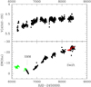 |
Fig. 4 Evolution with time of EW(Hα) (red stars from this paper, black dots from Nazé et al. 2019, green crosses from Zharikov et al. 2013) and V magnitude from ASAS-SN (“bb” camera only). Two dotted lines indicate the time of pointed X-ray observations (see Sect. 4). |
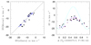 |
Fig. 5 Left: comparison between Hα velocities derived through three different methods, with the velocities derived by the mirror method as ordinates and those derived from moments (black dots) and two-Gaussian correlation (blue stars) as abscissae. The dotted diagonal indicates equality. Right: derived velocities phased with the average ephemeris of Bjorkman et al. (2002). Symbols are black dots for the centroid derived from moments, blue stars for velocities derived from the two-Gaussian correlation, and red crosses for velocities derived by the mirror method. The dotted cyan line provides the orbital solution of Bjorkman et al. (2002). |
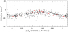 |
Fig. 6 Comparison of first-order moments derived for Hα in amateur spectra taken between October 2014 and January 2019 (black crosses) and in TIGRE data (red points). |
3.2 Tomography
We performed a tomographic analysis of the Hα line recorded by TIGRE in the same way as in Nazé et al. (2019). This technique assumes that the line profile variations are only due to our changing viewing angle because of the orbital motion (Horne 1991). Therefore, the emitting gas is stationary in the rotating frame of the binary, and each emitting parcel is associated with a specific (vx, vy) pair, considering an x-axis pointing from the primary to the secondary and a y-axis in the direction of the secondary motion. At any phase, the radial velocity of an emitting parcel recorded by a terrestrial observer will then be v(ϕt) = −vx cos(2πϕt) + vy sin(2πϕt) + vz. In this formulation, ϕt is zero at the conjunction with the secondary in front, so that it is shifted with respect to the orbital phase ϕ based on the ephemeris of Bjorkman et al. (2002): ϕt = ϕ + 0.25. Our Doppler tomography method further uses a Fourier-filtering to suppress some unwanted artifacts (Horne 1991; Rauw et al. 2002, 2005). The resulting Doppler map, shown in Fig. 10, provides the positions of emitting parcels in the velocity space considering that they remain stationary in the rotating frame of the binary. We may note that the tomographic map derived from Hα spectra taken by amateurs in 2018 (see Nazé et al. 2019 for the list) appears very similar to that derived from the TIGRE data alone, showing that the map appearance is not an artifact that is due to a peculiar sampling, for instance.
In this map, the Be disk appears as a large annular region encompassing the stars, with an outer radius slightly larger than 200 km s−1 and an inner radius <50 km s−1. The maximum intensities (delineated by the dark blue and magenta contours in Fig. 10) occur at a radius of ~100 km s−1, with a radial drop in intensity on either side. An additional drop in azimuth indicates a small asymmetry: the maximum intensities occur near the line joining the two stars and decrease in other directions. Compared to previous years (Zharikov et al. 2013; Nazé et al. 2019), the disk map in 2018 appears similar to the map recorded in 2016 or 2017. The Doppler map strongly differs, however, with the very asymmetric and thin partial ring of emission observed before 2015 when the Hα emission was much weaker.
Tomographic maps of other emission lines were also calculated (Hβ, H I λ8545, 8598 Å, Fe II λ 5317 Å, O I λ 7771–7775 Å). The resulting maps were similar to that of Hα, although they were noisier because these emissions are weaker.
4 High-energy emission
In the X-rayrange, π Aqr was first detected during the ROSAT all-sky survey and then during an XMM-Newton slew maneuver, but a detailed spectral description awaited a specific pointing by XMM-Newton in mid-November 2013 (Nazé et al. 2017). The latter observation showed that π Aqr exhibits the properties ofγ Cas stars: high temperature (kT ~11 keV), brightness intermediate between “normal” B stars and X-ray binaries ( erg cm−2 s−1, log [LX∕LBOL] ~−5.5), a fluorescent iron line in the iron complex at 6.7 keV, and variability. In this section, we derive the X-ray properties exhibited by π Aqr in 2018, and examine them in light of the simultaneous optical monitoring. We also compare them to the older X-ray data.
4.1 Spectral fitting
Count rates (Table 3) already provide some information on the X-ray properties of π Aqr, notably indicating significant variability (constancy is rejected with a significance level well below 0.1%). However, to study the system in more detail, the X-ray spectral distribution should be analyzed (Fig. 11). To this aim, we used Xspec v12.9.1p and considered reference solar abundances from Asplund et al. (2009). A visual examination of the spectra reveals that despite precautions (see Sect. 2.2), the spectra appear somewhat erratic or very noisy below 0.5 keV. These spectral bins were therefore not considered in our spectral fitting. As is usual for massive stars, we used an absorbed optically thin thermal emission model of the type tbabs × phabs × apec. The first absorption component represents the interstellar contribution, fixed to 3.6 × 1020 cm−2 (Nazé & Motch 2018), while the second accounts for additional local absorption. A single thermal component was used because this is sufficient to reach a good fit. Nazé et al. (2017) added a Gaussian line to account for the fluorescent iron line, but the low signal-to-noise ratio (S/N) of Swift spectra (compared to XMM-Newton data) renders this addition unnecessary.
We performed several fitting trials. First, we simultaneously fit all 30 Swift spectra with the same model. The reduced χ2 of the best fit reached a rather high value (1.80), which could be expected in view of the significant count rate changes from one observation to the next. We then kept the same temperature and absorbing column for all spectra, but allowed for different normalization factors. At 1.24, the reduced χ2 was much improved. The best-fit local column was (5.6 ± 0.5) × 1022 cm−2 and the best-fit temperature 16.5 keV, with a 68% (1σ) confidence interval of 13.2–21.0 keV. A last simultaneous fitting considered only the temperature as common to all data. It yielded an even better reduced χ2 (0.93), with a best-fit temperature of 14.8 keV (with a 68% confidence interval of 12.2–18.4 keV).
We then performed individual fittings, with local absorbing column, temperature, and normalization factor as free parameters. However, the fits often meandered because of the low S/N, resulting in unrealistic large error bars on the derived fluxes. We therefore decided to fix the temperature to 14.8 keV, as found in the simultaneous fitting, and found that the fit quality remained very similar (with a small modification of the second decimal of the reduced χ2 at most). Table 3 reports the results of this fitting procedure. When the temperature was instead fixed to 11.0 keV, as found from XMM-Newton data, the results were only marginally affected, with a second decimal change of the reduced χ2, for example. As a check, we compared the observed fluxes derived from this constrained fitting with the count rates (i.e., values derived without any fitting), and found a good correlation between them (ρ = 70%). As a second check, we also fit spectra obtained from the online tool (see footnote 1 in Sect. 2.2), and their results agree well with those derived from locally processed spectra. We therefore report in Table 3 only the latter.
Following recommendations of the XRT team for such bright sources (see also Nazé et al. 2018), the spectral fitting was also performed considering the possibility of energy scale offsets (command “gain fit” under Xspec, with slope fixed to 1). However, not only did the spectral parameters agree with those found from the usual fitting, but (1) the χ2 improvement was marginal, (2) very different offset values provided very similar statistics, and (3) offset valuesappeared not significant because they agreed with zero within the errors (or twice these 1σ errors). Because thisadjustment provided no significant improvement on the fits, we discuss only the fits achieved without these offsets here.
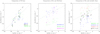 |
Fig. 7 Comparison of first-order moments of Hα to those of other lines. |
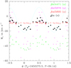 |
Fig. 8 Evolution with phase of first-order moments of Hα and other lines. The dotted cyan line provides the orbital solution of Bjorkman et al. (2002). The velocities of a non-varying interstellar line are shown in red to provide a comparison point. |
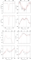 |
Fig. 9 Comparison of spectra taken at two different phases (25 August 2018, ϕ = 0.08, shown as thesolid black line, and 29 September 2018, ϕ = 0.50, shown as the red dotted line) around selected lines. The vertical lines indicate the expected companion velocity for the orbital solution of Bjorkman et al. (2002). |
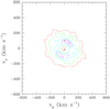 |
Fig. 10 Doppler map for Hα in 2018. The magenta, blue, cyan, green, and red contours correspond to amplitudes of 95, 80, 65, 50, and 35% of the maximum intensity. The two crosses indicate the velocities of the secondary (top) and primary (bottom) according to the semi-amplitudes K derived by Bjorkman et al. (2002). The maps correspond to a slice at vz = − 10 km s−1, the mean value in RV of the system; values of +10 or 0 km s−1 provide similar results, however. |
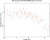 |
Fig. 11 Two X-ray spectra of π Aqr recorded by Swift, showing the intense emission at high energies at all times, but also clear variations. |
4.2 Behavior in 2018
During the 2018 campaign, the observed X-ray flux of π Aqr varied from 0.7 to 2.1 × 10⁻¹¹ erg cm−2 s−1 (Table 3). Normalization factors varied by a larger factor (3.2 versus 2.9) because the absorbing column also changed. However, the low-energy bins have low S/Ns and are therefore less reliable: while the local column seems to change (see previous section), its error bar remains large and caution should be taken when interpreting it. We may nevertheless note the presence of possible high-absorption events. This is not unusual for γ Cas stars (Hamaguchi et al. 2016), but they generally corresponded to times of lower (observed) X-ray fluxes. In our data, no strong correlation exists between absorbing column and fluxes: the correlation coefficient ρ is positive but only amounts to 12% when columns are compared to the observed fluxes (Fig. 12) and 46% when the noisier absorption-corrected fluxes are considered.
Figure 13 further shows the evolution of the X-ray fluxes and local absorbing columns with time and orbital phase: no coherent behavior is detected. Furthermore, in the same figure, the flux variations are compared with the evolution of the strength of the Hα line, which is a diagnostic of the disk properties. During 2018, the line strength slowly increased with time, the EW passed from –22 to –24.5 Å. In contrast, the X-ray fluxes do not display any obvious trend with time, neither does the local absorbing column: both rather seem to fluctuate continuously. The right panel of Fig. 13 directly compares X-ray fluxes and EWs when the X-ray exposures are associated with the closest optical spectra (see the last column of Table 2; averages were used when two X-ray datasets corresponded to one optical spectrum or vice versa). The figure shows large scatter. The correlation coefficient between these two parameters is only 15%, which demonstrates the absence of a strong and direct correlation between X-ray flux and Hα emission strength. Regardless of the time, the range in flux values remains rather constant. Similarly, no coherent behavior is found with phase for optical and X-ray diagnostics, despite a rather high disk inclination (50–75°, with 70° favored, see Bjorkman et al. 2002). The absence of (strong) orbital effects underlines that Hα and X-ray emission processes are independent from the presence of a companion. It may further be related to the fact that the disk now lacks the strong asymmetry noted in earlier data (see Sect. 3.2 and Nazé et al. 2019).
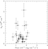 |
Fig. 12 Comparison between the local absorbing columns and the observed fluxes. |
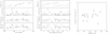 |
Fig. 13 Evolution with time (left) or orbital phase (middle, using an average ephemeris from Bjorkman et al. 2002) of the X-ray fluxes, best-fit local absorbing columns, and EWs of Hα in 2018 for π Aqr. The right panel directly compares the EW of Hα measured on TIGRE spectra and the observed X-ray flux of the closest Swift exposure(s). |
4.3 Long-term behavior
Examining the behavior of π Aqr on longer timescales implies a comparison with previous X-ray observations that were taken by ROSAT and XMM-Newton, although only the pointed XMM-Newton exposure (taken on HJD = 2 456 614.422) provided spectral information (Nazé et al. 2017; Nazé & Motch 2018). The best-fit temperature found for Swift spectra is only slightly higher than the temperature found for the pointed XMM-Newton observation (14.8 or 16.5 keV versus ~11.0 keV). Considering the error bars, this difference is marginal: it is only at the 2σ level. In addition, the fit quality does not significantly change when the XMM-Newton temperature is used to fit the Swift data. The available data therefore do not suggest strong temperature variations in the hot plasma of π Aqr.
The local absorbing columns found in individual fits vary between 1020 and 3 × 1022 cm−2, a wide range that encompasses the XMM-Newton value (2 × 1021 cm−2). However, the Swift observations are 1 ks snapshots, while the XMM-Newton exposure was 55 ks long. During this exposure, the source brightness varied by a factor 2–3 over a few hours (see Fig. 2 of Nazé et al. 2017), a similar range as observed in Swift observations over several months. It therefore appears meaningful to compare the column found from the fitting the whole XMM-Newton exposure with that derived from the simultaneous fitting of all Swift spectra (5.6 × 1022 cm−2, see above). The local absorption is then found to be significantly (7σ) higher in Swift observations. Because no systematic difference between Swift and XMM-Newton (i.e., due to imperfect cross-calibration) has been reported, this absorption difference is most probably real.
In the Swift data, π Aqr displays an average flux of  (1.38 ± 0.04) × 10−11 erg cm−2 s−1. In the pointed XMM-Newton exposure, π Aqr showed
  10−11 erg cm−2 s−1 (Nazé & Motch 2018), therefore the X-ray level of π Aqr appears somewhat higher in 2018 than in2013. π Aqr was also detected by XMM-Newton on HJD = 2 453 145.919 during slew maneuvers. It is reported in the slew survey clean catalog, v2.0, as XMMSL2 J222517.0+012226 with an EPIC-pn count rate of 2.8 ± 1.1 cts s−1 in 0.2–12. keV. In the same energy band, the 3XMM-DR8 catalog reports the π Aqr detection from the pointed observation as 3XMM J222516.6+012238 with an EPIC-pn4 count rate of 2.242 ± 0.008 cts s−1. The slew count rate is therefore formally 25% higher than that in the pointed observation, but it is indistinguishable in view of its large error bar. Nazé et al. (2017) also compared the ROSAT detection and the pointed XMM-Newton observation. The ROSAT count rate formally indicates a flux in the 0.1–2.0 keV energy band that is ~30% lower, but the values were compatible at 3σ considering the rather large ROSAT error.
Overall, the average X-ray level of π Aqr thus seems to vary in a moderate way (up to 40%) over time. However, the short-term variations are of a large amplitude: a factor of 3 during the 2018 Swift monitoring, and a factor of 2–3 during the 55 ks XMM-Newton exposure. A random snapshot of π Aqr, such as the XMM-Newton slew observation or any individual Swift exposure, therefore has a high probability of deviating from the average by a non-negligible amount. When we take these short-term variations into account and consider the similar average levels, the only possible conclusion is that the X-ray emission level of π Aqr has not significantly changed over time.
In parallel, the disk of π Aqr has undergone dramatic changes, as traced by its Hα line. During the Swift monitoring, the Hα line was very strong (EW ~−23Å) and the disk appeared quite symmetric (see Sect. 3.2). In contrast, at the time of the pointed XMM-Newton observation, the Hα emission was much weaker, and the photospheric absorption was clearly detectable (Nazé et al. 2019). The closest amateur spectrum, taken only one day later, has EW = −1.73Å (Nazé et al. 2019), with EW estimated in the same way as in previous section. Furthermore, the disk was then much more asymmetric and much less extended (Nazé et al. 2019). In this context, it is also important to note that ASAS-SN photometry indicates a simultaneous overall brightening of π Aqr by ~0.4 mag in V band (Fig. 4).
Unfortunately, much less information is available for the time of the other X-ray observations. The ROSAT survey observations took place in 1990–1991, when π Aqr was rapidly transitioning from an active to a quiet phase (Bjorkman et al. 2002): very precise observing dates would be needed for a meaningful statement, but they are not available. The EW of the Hα line at the time of the XMM-Newton slew observation (HJD = 2 453 145.919) is unknown: the closest spectrum, taken three months later, is reported by Zharikov et al. (2013) with a moderate EW of –3.53 Å.
To further specify the extent of the disk variation between 2013 and 2018, we now try to quantitatively assess the disk size. The separation between the violet and red peaks of the Hα emission profile can be related to the radius of the emission zone if the disk rotation is Keplerian (Zamanov et al. 2019). When we use the observed separation (~320 km s−1 in 2013 and ~140 km s−1 in 2018, see Nazé et al. 2019) as well as the projected rotational velocity of the star (v sini ~ 250 km s−1) and stellar radius (R* = 6.1 R⊙) from Bjorkman et al. (2002), Eq. (2) of Zamanov et al. (2019) yields a radius for the emission region of 2.4 R* = 14.9 R⊙ in 2013 and 12.8 R* = 77.8 R⊙ in 2018, that is, an increase by a factor of 5 in the extension of the Hα emission region. The separation between the Be star and its companion was determined to be a sini = 0.96 AU = 207 R⊙, or 220 R⊙ for the favored inclination, 70° (Bjorkman et al. 2002). This means that the orbital separation was 14.8 times the disk radius (as determined from the Hα emission) in2013, but only 2.8 times that radius in 2018. In Sect. 3.1 we found that the velocity amplitude of the primary in 2018 was half the value reported by Bjorkman et al. (2002), which implies a separation a smaller by 7%. For the same inclination, this separation would correspond to 13.7 Rdisk in 2013 or 2.6 Rdisk in 2018. Because the absorbing column appears larger when the disk emission is stronger, this may readily be interpreted in terms of more material being available along the line of sight to emit as well as to absorb X-rays (the latter being observed while the former is not).
How does π Aqr compare with other γ Cas stars? Unfortunately, only two such stars were simultaneously monitored in X-ray and optical domains. The first is γ Cas itself. It simultaneously brightens at optical and X-ray wavelengths, as demonstrated by the clear correlation between the X-ray fluxes and the V-band magnitudes found by Robinson et al. (2002) and Motch et al. (2015), apparently without delay, and we recall that Smith et al. (2012) found that γ Cas brightens in the optical as its disk emission strengthens. Furthermore, it also exhibited an increased local absorption of X-rays when its Hα emission was stronger (Smith et al. 2012). The second example is HD 45314. This star was monitored during large variations of its disk by Rauw et al. (2018): the strong Hα weakening (EW passing from –22.6 to –8.5 Å), although not as extreme as for π Aqr, corresponded to a flux decrease in X-rays of an order of magnitude ( changing from 11. to 1.2 × 10⁻¹³ erg cm−2 s−1). This was interpreted as reflecting the fact that much less disk material was then available for X-ray emission. No obvious relationship was found between local absorbing column and X-ray flux or EW(Hα), however, but the spectral model was different in the minimum flux stage because the thermal emission was also much softer at the time, rendering a direct comparison of the absorption of the hard component more awkward. While the variation in absorption seems similar to that recorded in γ Cas, the behavior of π Aqr therefore surprisingly departs from that of its fellow γ Cas stars by lacking the large change in X-ray flux observed for both γ Cas and HD 45314 in reaction to the disk variations (traced by Hα emission and/or V-band magnitudes).
Theoretically, both scenarios under consideration for explaining the γ Cas phenomenon (accretion and star-disk interactions) expect changes in the disk to lead to changes in X-ray emission level. This is quite obvious for the star-disk interaction scenario because the X-ray emission directly arises in or close to the disk and is therefore expected to depend sensitively on its properties. However, the emission is assumed to take place close to the star in this model, therefore the disk density in the inner regions could be more important than the disk extent itself.
On the other hand, scenarios involving accretion onto a compact object could be more sensitive to variations in the outer regions of the disk. Be X-ray binaries display changes in their X-ray emission when the disk varies (e.g., type II outbursts, see Reig 2011). Some delay may be involved in this case, however. For accretion onto a neutron star in the propeller stage, Postnov et al. (2017) estimated a delay of  (where RL is the Roche-lobe radius of the neutron star) for free-fall time inside the neutron star’s Roche lobe. Considering Kepler’s third law 4π2 a3 = P2G(MBe + MNS) and RL ~ 0.5aMNS∕(MBe + MNS) (Eq. (17) in Postnov et al. 2017) yields a delay ~ P∕8π or 3 d for π Aqr. To this should be added the time for any stellar mass-loss or outer disk material to flow to the Roche lobe of the neutron star. However, because we focus here on the slow and large Hα variations, which took years (see Fig. 4), this delay is negligible when we compare the 2013 and 2018 epochs. In this context, it may be useful to note that for the mass ratio of 0.16 determined by Bjorkman et al. (2002), the Roche-lobe radius of the primary reaches 54% of the separation, or 120 R⊙, so that no overflow seems possible even in 20185. Disk Roche-lobe overflow therefore seems prohibited at all times. Instead, we might imagine that the stellar wind is responsible for accretion instead of the disk material. However, a strong decoupling between disk (as traced by the Hα line in this scenario) and wind (as traced by X-rays in this scenario) is then required in π Aqr but not in the other two γ Cas stars to explain observations. Finally, we may note that orbital modulation of the X-ray emission appears widespread for systems with accreting white dwarfs (e.g., Szkody et al. 1996; Patterson et al. 1998; Parker et al. 2005), although none is observed here.
5 Conclusions
We conducted a monitoring of π Aqr in 2018 in the optical and X-ray domains. At the time, π Aqr appeared very active, reaching emission levels that had not been seen since 1990 (Nazé et al. 2019). The Hα line shows clear velocity variations, which can be phased with the ephemeris of Bjorkman et al. (2002). However, the positive velocity values recorded two decades ago (when the Hα line was in absorption) are not seen during our 2018 monitoring (with the same line being in emission). As a consequence, the velocity amplitude has been halved. This does not seem to be linked to a bias introduced by the companion emission line or its influence on the disk structure.
X-ray variations by a factor of 3 are recorded during our monitoring. However, they show no obvious link with orbital phase or with Hα line strength. They most probably reflect the short-term X-ray variability seen in γ Cas stars. Comparing the properties to older X-ray detections, we find that the overall X-ray flux level of π Aqr remains stable, despite an increase in optical brightness (V magnitude) and large changes in disk structure and extent (as traced by the Hα line). An increase in absorbing column is potentially detected, however.
This stability appears at odds with observations of other γ Cas stars, which showed clear correlations between their X-ray and optical (EW(Hα) or V-magnitude) emissions, and also possibly with scenarios proposed to explain the γ Cas behavior. The surprising behavior of π Aqr therefore points toward a missing ingredient in the considered scenarios. Unfortunately, it is quite difficult to point out the exact reason for this discrepancy because the number of γ Cas stars that are monitored in optical and X-rays is quite limited for the moment. Such monitoring should therefore be performed for more stars to assess exactly whether π Aqr is truly an exception or if a range of behaviors are actually present in γ Cas stars, with π Aqr and γ Cas/HD 45314 at the extremes. Extending the wavelength coverage to the NIR and UV also seems relevant to further assess the wind and circumstellar material as well as the properties of the companion.
Acknowledgements
We thank C. Motch, R. Lopes de Oliveira, and A. Miroshnichenko for fruitful discussions. Y.N. and G.R. acknowledgesupport from the Fonds National de la Recherche Scientifique (Belgium), the Communauté Française de Belgique, the European Space Agency (ESA) and the Belgian Federal Science Policy Office (BELSPO) in the framework of the PRODEX Programme (contract XMaS). We are grateful to the Swift team, especially Kim Page, for their help and good advice. ADS and CDS were used for preparing this document.
References
- Asplund, M., Grevesse, N., Sauval, A. J., & Scott, P. 2009, ARA&A, 47, 481 [NASA ADS] [CrossRef] [Google Scholar]
- Baade, D., Pigulski, A., Rivinius, T., et al. 2018, A&A, 610, A70 [NASA ADS] [CrossRef] [EDP Sciences] [Google Scholar]
- Bailer-Jones, C. A. L., Rybizki, J., Fouesneau, M., Mantelet, G., & Andrae, R. 2018, AJ, 156, 58 [NASA ADS] [CrossRef] [Google Scholar]
- Bjorkman, K. S., Miroshnichenko, A. S., McDavid, D., & Pogrosheva, T. M. 2002, ApJ, 573, 812 [NASA ADS] [CrossRef] [Google Scholar]
- Cantiello, M., Langer, N., Brott, I., et al. 2009, A&A, 499, 279 [NASA ADS] [CrossRef] [EDP Sciences] [Google Scholar]
- Evans, P. A., Beardmore, A. P., Page, K. L., et al. 2009, MNRAS, 397, 1177 [NASA ADS] [CrossRef] [Google Scholar]
- Hamaguchi, K., Oskinova, L., Russell, C. M. P., et al. 2016, ApJ, 832, 140 [NASA ADS] [CrossRef] [Google Scholar]
- Hinkle, K., Wallace, L., Valenti, J., & Harmer, D. 2000, Visible and Near Infrared Atlas of the Arcturus Spectrum 3727-9300 A, eds. K. Hinkle, L. Wallace, J. Valenti, & D. Harmer (San Francisco: ASP) [Google Scholar]
- Horne, K. 1991, in Fundamental Properties of Cataclysmic Variable Stars: 12th North American Workshop on Cataclysmic Variables and Low Mass X-ray Binaries, ed. A. W. Shafter (San Diego: SDSU Press), 23 [Google Scholar]
- Mittag, M., Hempelmann, A., González-Pérez, J. N., & Schmitt, J. H. M. M. 2010, Adv. Astron., 2010 101502 [NASA ADS] [CrossRef] [Google Scholar]
- Motch, C., Lopes de Oliveira, R., & Smith, M. A. 2015, ApJ, 806, 177 [NASA ADS] [CrossRef] [Google Scholar]
- Murakami, T., Koyama, K., Inoue, H., & Agrawal, P. C. 1986, ApJ, 310, L31 [NASA ADS] [CrossRef] [Google Scholar]
- Nazé, Y., & Motch, C. 2018, A&A, 619, A148 [NASA ADS] [CrossRef] [EDP Sciences] [Google Scholar]
- Nazé, Y., Rauw, G., & Cazorla, C. 2017, A&A, 602, L5 [NASA ADS] [CrossRef] [EDP Sciences] [Google Scholar]
- Nazé, Y., Ramiaramanantsoa, T., Stevens, I. R., et al. 2018, A&A, 609, A81 [NASA ADS] [CrossRef] [EDP Sciences] [Google Scholar]
- Nazé, Y., Rauw, G., Guarro Fló, J., et al. 2019, New Astron., 73, 101279 [CrossRef] [Google Scholar]
- Nemravová, J., Harmanec, P., Koubský, P., et al. 2012, A&A, 537, A59 [NASA ADS] [CrossRef] [EDP Sciences] [Google Scholar]
- Parker, T. L., Norton, A. J., & Mukai, K. 2005, A&A, 439, 213 [NASA ADS] [CrossRef] [EDP Sciences] [Google Scholar]
- Patterson, J., Richman, H., Kemp, J., et al. 1998, PASP, 110, 403 [NASA ADS] [CrossRef] [Google Scholar]
- Postnov, K., Oskinova, L., & Torrejón, J. M. 2017, MNRAS, 465, L119 [NASA ADS] [CrossRef] [Google Scholar]
- Rauw, G., Crowther, P. A., Eenens, P. R. J., Manfroid, J., & Vreux, J.-M. 2002, A&A, 392, 563 [NASA ADS] [CrossRef] [EDP Sciences] [Google Scholar]
- Rauw, G., Crowther, P. A., De Becker, M., et al. 2005, A&A, 432, 985 [NASA ADS] [CrossRef] [EDP Sciences] [Google Scholar]
- Rauw, G., Nazé, Y., Smith, M. A., et al. 2018, A&A, 615, A44 [NASA ADS] [CrossRef] [EDP Sciences] [Google Scholar]
- Reig, P. 2011, Ap&SS, 332, 1 [NASA ADS] [CrossRef] [Google Scholar]
- Robinson, R. D., Smith, M. A., & Henry, G. W. 2002, ApJ, 575, 435 [NASA ADS] [CrossRef] [Google Scholar]
- Schmitt, J. H. M. M., Schröder, K.-P., Rauw, G., et al. 2014, Astron. Nachr., 335, 787 [NASA ADS] [CrossRef] [Google Scholar]
- Shafter, A. W., Szkody, P., & Thorstensen, J. R. 1986, ApJ, 308, 765 [NASA ADS] [CrossRef] [Google Scholar]
- Sigut, T. A. A., & Patel, P. 2013, ApJ, 765, 41 [NASA ADS] [CrossRef] [Google Scholar]
- Szkody, P., Long, K. S., Sion, E. M., et al. 1996, ApJ, 469, 834 [NASA ADS] [CrossRef] [Google Scholar]
- Smith, M. A., & Robinson, R. D. 1999, ApJ, 517, 866 [NASA ADS] [CrossRef] [Google Scholar]
- Smith, M. A., Robinson, R. D., & Corbet, R. H. D. 1998, ApJ, 503, 877 [NASA ADS] [CrossRef] [Google Scholar]
- Smith, M. A., Lopes de Oliveira, R., Motch, C., et al. 2012, A&A, 540, A53 [NASA ADS] [CrossRef] [EDP Sciences] [Google Scholar]
- Smith, M. A., Lopes de Oliveira, R., & Motch, C. 2016, Adv. Space Res., 58, 782 [NASA ADS] [CrossRef] [Google Scholar]
- Zamanov, R., Stoyanov, K. A., Wolter, U., Marchev, D., & Petrov, N. I. 2019, A&A, 622, A173 [NASA ADS] [CrossRef] [EDP Sciences] [Google Scholar]
- Zharikov, S. V., Miroshnichenko, A. S., Pollmann, E., et al. 2013, A&A, 560, A30 [NASA ADS] [CrossRef] [EDP Sciences] [Google Scholar]
After multiplication by minus the wavelength step, to have the usual definition of positive EWs for absorptions and negative EWs for emissions.
Nazé et al. (2017) incorrectly assumed that the slew count rates refer to all EPIC and not to the EPIC-pn camera alone.
If we were to keep the secondary velocity amplitude of Bjorkman et al. (2002) but considered half the value for the primary amplitude (see Sect. 3.1), the mass ratio would then be halved and the Roche-lobe radius of the primary increased to 150 R⊙.
All Tables
All Figures
|
Fig. 1 Spectrum of π Aqr taken by TIGRE on 10 July 2018, after correction of the telluric lines. |
| In the text | |
|
Fig. 2 Evolution with time of zeroth-order moments (EWs) for hydrogen, He I, and metallic lines. In these panels, higher emissions (absorptions) are toward the top (bottom). For Hα, the values derived from amateur data reported by Nazé et al. (2019) are also shown as small red crosses. |
| In the text | |
|
Fig. 3 Evolution with time or phase of the V∕R for the Hα and Hβ lines. |
| In the text | |
|
Fig. 4 Evolution with time of EW(Hα) (red stars from this paper, black dots from Nazé et al. 2019, green crosses from Zharikov et al. 2013) and V magnitude from ASAS-SN (“bb” camera only). Two dotted lines indicate the time of pointed X-ray observations (see Sect. 4). |
| In the text | |
|
Fig. 5 Left: comparison between Hα velocities derived through three different methods, with the velocities derived by the mirror method as ordinates and those derived from moments (black dots) and two-Gaussian correlation (blue stars) as abscissae. The dotted diagonal indicates equality. Right: derived velocities phased with the average ephemeris of Bjorkman et al. (2002). Symbols are black dots for the centroid derived from moments, blue stars for velocities derived from the two-Gaussian correlation, and red crosses for velocities derived by the mirror method. The dotted cyan line provides the orbital solution of Bjorkman et al. (2002). |
| In the text | |
|
Fig. 6 Comparison of first-order moments derived for Hα in amateur spectra taken between October 2014 and January 2019 (black crosses) and in TIGRE data (red points). |
| In the text | |
|
Fig. 7 Comparison of first-order moments of Hα to those of other lines. |
| In the text | |
|
Fig. 8 Evolution with phase of first-order moments of Hα and other lines. The dotted cyan line provides the orbital solution of Bjorkman et al. (2002). The velocities of a non-varying interstellar line are shown in red to provide a comparison point. |
| In the text | |
|
Fig. 9 Comparison of spectra taken at two different phases (25 August 2018, ϕ = 0.08, shown as thesolid black line, and 29 September 2018, ϕ = 0.50, shown as the red dotted line) around selected lines. The vertical lines indicate the expected companion velocity for the orbital solution of Bjorkman et al. (2002). |
| In the text | |
|
Fig. 10 Doppler map for Hα in 2018. The magenta, blue, cyan, green, and red contours correspond to amplitudes of 95, 80, 65, 50, and 35% of the maximum intensity. The two crosses indicate the velocities of the secondary (top) and primary (bottom) according to the semi-amplitudes K derived by Bjorkman et al. (2002). The maps correspond to a slice at vz = − 10 km s−1, the mean value in RV of the system; values of +10 or 0 km s−1 provide similar results, however. |
| In the text | |
|
Fig. 11 Two X-ray spectra of π Aqr recorded by Swift, showing the intense emission at high energies at all times, but also clear variations. |
| In the text | |
|
Fig. 12 Comparison between the local absorbing columns and the observed fluxes. |
| In the text | |
|
Fig. 13 Evolution with time (left) or orbital phase (middle, using an average ephemeris from Bjorkman et al. 2002) of the X-ray fluxes, best-fit local absorbing columns, and EWs of Hα in 2018 for π Aqr. The right panel directly compares the EW of Hα measured on TIGRE spectra and the observed X-ray flux of the closest Swift exposure(s). |
| In the text | |
Current usage metrics show cumulative count of Article Views (full-text article views including HTML views, PDF and ePub downloads, according to the available data) and Abstracts Views on Vision4Press platform.
Data correspond to usage on the plateform after 2015. The current usage metrics is available 48-96 hours after online publication and is updated daily on week days.
Initial download of the metrics may take a while.