| Issue |
A&A
Volume 631, November 2019
|
|
|---|---|---|
| Article Number | A169 | |
| Number of page(s) | 14 | |
| Section | Planets and planetary systems | |
| DOI | https://doi.org/10.1051/0004-6361/201935364 | |
| Published online | 18 November 2019 | |
Ground-based optical transmission spectrum of the hot Jupiter HAT-P-1b★
1
Anton Pannekoek Institute for Astronomy, University of Amsterdam,
Science Park 904,
XH 1098
Amsterdam,
The Netherlands
e-mail: This email address is being protected from spambots. You need JavaScript enabled to view it.
2
CASA, University of Colorado,
389 UCB,
Boulder,
CO
80309-0389,
USA
3
Department of Astronomy and Astrophysics, University of Chicago,
Chicago,
IL
60637,
USA
4
Department of Astronomy and Astrophysics, University of California,
Santa Cruz,
CA
95064,
USA
5
Space Telescope Science Institute,
3700 San Martin Drive,
Baltimore,
MD
21218,
USA
6
NOAO, Gemini Observatory,
950 North Cherry Ave.,
Tucson,
AZ
85719,
USA
Received:
25
February
2019
Accepted:
17
September
2019
Abstract
Context. Time-series spectrophotometric studies of exoplanets during transit using ground-based facilities are a promising approach to characterize their atmospheric compositions.
Aims. We aim to investigate the transit spectrum of the hot Jupiter HAT-P-1b. We compare our results to those obtained at similar wavelengths by previous space-based observations.
Methods. We observed two transits of HAT-P-1b with the Gemini Multi-Object Spectrograph (GMOS) instrument on the Gemini North telescope using two instrument modes covering the 320–800 and 520–950 nm wavelength ranges. We used time-series spectrophotometry to construct transit light curves in individual wavelength bins and measure the transit depths in each bin. We accounted for systematic effects. We addressed potential photometric variability due to magnetic spots in the planet’s host star with long-term photometric monitoring.
Results. We find that the resulting transit spectrum is consistent with previous Hubble Space Telescope (HST) observations. We compare our observations to transit spectroscopy models that marginally favor a clear atmosphere. However, the observations are also consistent with a flat spectrum, indicating high-altitude clouds. We do not detect the Na resonance absorption line (589 nm), and our observations do not have sufficient precision to study the resonance line of K at 770 nm.
Conclusions. We show that even a single Gemini/GMOS transit can provide constraining power on the properties of the atmosphere of HAT-P-1b to a level comparable to that of HST transit studies in the optical when the observing conditions and target and reference star combination are suitable. Our 520–950 nm observations reach a precision comparable to that of HST transit spectra in a similar wavelength range of the same hot Jupiter, HAT-P-1b. However, our GMOS transit between 320–800 nm suffers from strong systematic effects and yields larger uncertainties.
Key words: planets and satellites: atmospheres / planets and satellites: individual: HAT-P-1b / techniques: spectroscopic
A table of the chromatic light curves and the reduced spectra are only available at the CDS via anonymous ftp to cdsarc.u-strasbg.fr (130.79.128.5) or via http://cdsarc.u-strasbg.fr/viz-bin/cat/J/A+A/631/A169
e-mail: This email address is being protected from spambots. You need JavaScript enabled to view it.
Current address: Palo Alto, CA, USA.
© ESO 2019
1 Introduction
The atmospheres of transiting hot exoplanets have been probed through time-series transit spectroscopy, for instance, using data from the Hubble Space Telescope (HST, e.g., Charbonneau et al. 2002; Vidal-Madjar et al. 2003; Deming et al. 2013; Sing et al. 2016; Arcangeli et al. 2018). From the ground, transit studies have used multi-object spectrographs (MOS; e.g., Bean et al. 2010, 2011; Gibson et al. 2013b; Stevenson et al. 2014; Nikolov et al. 2016; Huitson et al. 2017; Rackham et al. 2017; Bixel et al. 2019; Espinoza et al. 2019) and long-slit spectrographs in low-resolution mode (e.g., Sing et al. 2012; Murgas et al. 2014, 2019; Nortmann et al. 2016). Studies using ground-based high-resolution spectrographs (e.g., Redfield et al. 2008; Snellen et al. 2008; Nortmann et al. 2018) have also yielded information on the planetary atmospheres.
We here focus on the MOS technique, which relies on time-series spectrophotometry of the target star-planet system during transit. The objective, as with all time-series transit spectroscopy, is to measure the depth of a transit as a function of wavelength to extract a transit spectrum, which carries information about the contents of the planetary atmosphere. A reference star is typically observed in another MOS slit to help mitigate any spectrophotometric systematic effects. Long-slit spectrographs have also been used.
This work, along with the study by Huitson et al. (2017), is part of a transit spectroscopy survey using the Gemini/GMOS instrument that observed nine transiting exoplanets during a total of about 40 transits with high spectrophotometric precision in visible wavelengths. The results from Huitson et al. (2017) have been used by Bouma et al. (2019) along with other observations, including TESS transits, to detect transit timing variations of the hot Jupiter WASP-4b. The goal of the GMOS survey is to robustly estimate systematic effects and extract high-fidelity transit spectra for the target planets, ultimately constraining Rayleigh scattering and cloud deck prevalence in irradiated atmospheres. In this study, we focus on GMOS time-series transit spectroscopy observations of a well-studied hot Jupiter.
HAT-P-1b is one of the first hot Jupiters discovered with the transit technique (Bakos et al. 2007, Table 1). The host star, HAT-P-1, is reasonably bright, old (3.6 Gyr, Bakos et al. 2007), and inactive (e.g., Knutson et al. 2010; Nikolov et al. 2014). The equilibrium temperature of the planet’s day side is approximately 1300 K (assuming full irradiation redistribution to the night side; Nikolov et al. 2014). The Rossiter-McLaughlin effect for the system was observed by Johnson et al. (2008), who showed that the planet’s orbital axis is well aligned with the stellar spin axis, indicating a post-formation orbital evolution that preserves alignment. Another aspect of the system is the presence of an equal-mass stellar companion at an angular distance of 11.26′′ (V = 9.75, F8V).
The atmosphere of HAT-P-1b has been studied extensively in the past. Todorov et al. (2010) observed the planet’s secondary eclipses using broadband photometry at 3.6, 4.5, 5.8, and 8.0 μm with the IRAC instrument on Spitzer and concluded that the mid-infrared spectral energy distribution of the planet’s dayside is consistent with a black body. The secondary eclipse of the planet was also detected in the Ks band using the Long-slit Intermediate Resolution Infrared Spectrograph (LIRIS) on the William Herschel Telescope (WHT) (de Mooij et al. 2011). In the following years, investigators focused on transit spectroscopy studies using the HST with the Wide Field Camera 3 (WFC3) and the Space Telescope Imaging Spectrograph (STIS) instruments. Wakeford et al. (2013) used the G141 grism on the WFC3 to create a low-resolution (R ~70) transit spectrum in the wavelength range between 1.09 and 1.68 μm. These authors detected water absorption from the 1.4 μm at more than 5σ. Nikolov et al. (2014) used HST/STIS to extract a low-resolution transit spectrum between 0.29 and 1.03 μm. These observations yielded a detection of sodium at 0.589 μm at 3.3σ. Sing et al. (2016) summarized the HST observations and placed them in the context of Spitzer transit photometry observations at 3.6 and 4.5 μm, and of otherHST transit spectroscopy studies of hot Jupiters. Montalto et al. (2015) presented a very low-resolution transit spectrum in the visible range obtained with the Device Optimized for the Low Resolution (DOLORES) on the 3.6 m ground-based TelescopioNazionale Galileo (TNG). Potassium has been detected in the atmosphere of HAT-P-1b in transit using the Optical System for Imaging and low Resolution Integrated Spectroscopy (OSIRIS) on the Gran Telescopio Canarias (GTC) in tunable filter imaging mode near 766.5 nm (Wilson et al. 2015).
In this work, we measure the optical transit spectra we have obtained between 0.3 and 0.9 μm, using the GMOS-N instrument on the Gemini North telescope and discuss them in the context of previous HST/STIS and TNG/DOLORES results in the visible range. In Sect. 2 we present the our observational strategy and discuss the specifics of our data. Section 3 details our data reduction approach. Section 4 focuses on our treatment of the time series and the transit spectrum extraction. Section 5 discusses our data modeling and the implications of our results.
Parameters for the HAT-P-1 system.
2 Observations
2.1 GMOS transit spectroscopy
We observed two primary transits of HAT-P-1b using the Gemini Multi-Object Spectrograph (GMOS-N) instrument on the GeminiNorth telescope (Maunakea, Hawaii) on 2012 November 12 and on 2015 November 02 (Table 2). Our observing strategy is similar to that of Huitson et al. (2017) and to those of other earlier studies using this instrument (e.g., Gibson et al. 2013a,b; Stevenson et al. 2014; von Essen et al. 2017).
The goal of the observations was to perform accurate spectrophotometry of the target star (HAT-P-1, or BD+37 4734B). Therefore, we configured GMOS in its multi-object spectrograph mode (MOS) to observe the target and a suitable reference star (BD+37 4734A, the binary companion to the target, 11.26′′ separation). The target and reference stars have comparable spectral types and magnitudes (G0V with V = 9.87, and F8V with V = 9.75, respectively; Høg et al. 2000; Zacharias et al. 2013).
Both stars were observed through the same 30′′ long slit because they are close enough that a single slit provides sufficient sky coverage to assess the background. To mitigate any time-variable slit losses that could complicate our time-series analysis, we chose to use a wide slit (10′′). We ensured that the wavelength coverage was consistent between stars by selecting the position angle of the MOS slit mask to be equal to the PA between the two stars (74.3° E of N).
The transit observation in 2012 was performed with the R150 + G5306 grating combination (from now on, “the R150 transit”). The OG515_G0306 filter was used to block light at wavelengths shorter than ~520 nm, as well as to block out contamination from other orders. This yielded a wavelength coverage of 520 to 950 nm. The 2015 transit observation used the B600 + G5307 grating (the “B600 transit”), with a wavelength coverage of 320–800 nm. No blocking filter was used.
The ideal resolving power of the R150 observation is R = 631 at the blaze wavelength (717 nm), and for the B600 observation, it is R = 1688 at a blaze wavelength of 461 nm. These values assume a 0.5′′ wide slit (Hook et al. 2004, GMOS Online Manual), but our observations use a 10′′ wide slit and are seeing limited. The wavelength resolution we obtain is 2− 6× lower than the ideal values.
Our data were observed while GMOS was still operating with its e2v DD detectors. These are decommissioned in GMOS-N since February 2017. We reduced the read-out noise by windowing a region of interest (ROI) on the detector in covering both spectral traces, rather than reading the whole detector. A single ROI was used to cover both stellar spectra. In addition, we binned the detector output (1 × 2) in the cross-dispersion direction. The detector was read out with six amplifiers and with gains of approximately 2 e− /ADU in each amplifier (although the R150 spectral traces only cover four amplifiers). Exposure times were chosen to keep count levels between ~10 000 and 40 000 peak ADU and well within the linear regime of the CCDs (<50% of the full well of the detector). The total duration of the transit observations was 6 h 13 m (R150) and 5 h 44 m (B600). The transit duration of HAT-P-1b is 2 h 40 m, allowing sufficient out-of-transit sampling of the light curves.
Observations.
2.2 Long-term photometric monitoring of HAT-P-1
We obtained photometric observations in the Johnson-Cousins/Bessell B-band of HAT-P-1b using the Las Cumbres Observatory (LCO) global network of robotic telescopes (Brown et al. 2013). The network consists of 42 telescopes with mirrors with diameters of 40 cm, 1 m, and 2 m. The telescopes are spread across Earth in latitude and longitude, providing full sky coverage. Our 674 photometric observations cover eight months between 2016 April 25 and 2016 December 12 (one measurement every 8 h on average, weather permitting, with flexible scheduling). We used only the 40 cm and 1 m telescopes with the SBIG 4k × 4k imagers.
3 Data reduction
We based our data reduction on the custom GMOS transit spectroscopy pipeline discussed in detail in Huitson et al. (2017). We used this code to correct the raw images for gain and bias levels, to perform cosmic ray identification, to remove bad columns, to flat-field the data, and to correct for slit tilt (as needed), and finally, to extract the 1D spectra. We then applied corrections for additional time- and wavelength-dependent dispersion shifts between target and reference stars on the detector due to weather and airmass, for example. In this section we outline the main points of the pipeline and the additional corrections required by our data.
3.1 Extracting the time series
Cosmic rays were detected with 5σ clipping using a moving boxcar of 20 frames in time, where the value of a given pixel was compared to the values of the same pixel in the images obtained immediately before and after. The value of the flagged pixel was replaced by the median value of that pixel within the boxcar. The cosmic-ray removal flagged several percent of pixels per image frame.
The GMOS-N e2v detectors suffered from bad pixel columns, which we identified and excluded from our analysis. The pipeline flagged 1.9– 2.6% of columns as bad by comparing the out-of-slit counts within a given column with those of neighboring columns. The majority (~90%) of flagged columns are consistent between transits and typically occur in the transition regions between detector amplifiers. We saw no columns of shifted charge like those in the GMOS detector on the Gemini South telescope prior to July 2014, as reported by Huitson et al. (2017).
Flat-fielding should ideally not be necessary because our measurement is relative and we followed thecounts in the same set of pixels as a function of time. However, as the pointing changed throughout the night, the gravity vector on the instrument evolved, causing flexing. As a result, the spectral trace drifted over different detector pixels during the observation. Therefore, we tested our extraction with and without flat-fielding. We find that flat-fielding does not significantly affect the scatter of the resulting white-light curves, increasing it(B600) or decreasing it (R150) by several percent. For consistency, we chose to omit flat-fielding in both observations.
The HAT-P-1 transit spectrum observations do not suffer from spectral tilt. The sky lines on the image are parallel to the pixel columns. We therefore did not correct for it.
We applied the optimal extraction algorithm (Horne 1986) to obtain the 1D spectra. We tested a range of aperture sizes between 10 and 60 pixels in the cross-dispersion direction. We find that the lowest scatter in the out-of-transit light curves is produced by an aperture of 20 pixels for both observations.
3.1.1 Slit losses
Slit losses are caused by a combination of differential atmospheric dispersion and differential refraction (e.g., Sánchez-Janssen et al. 2014). For the airmass ranges in our study (Table 2), a separation of 11.26′′, and using Eq. (3) in Sánchez-Janssen et al. (2014), we estimate that the apparent shift in position due to differential refraction is between 0.002′′ and 0.009′′ (R150), and 0.002′′ and 0.016′′ (B600). This is much smaller than our 10′′ slit, and so it is unlikely that differential refraction plays a large role in our observations. Because the reference and target stars form an almost equal-mass binary, they have very similar spectral types, colors, and apparent brightness. Thus, differential atmospheric dispersion is also unlikely to play a large role for our observations. Any variations are likely to be gradual with time and would be accounted for by our instrumental effects corrections (e.g., Sect. 4.1, Eq. (2)).
Another aspect is that any time jitter in the position angle (PA) of the slit could introduce differential slit losses. No such variability is recorded in the FITS file headers, but low-level pointing changes cannot be completely ruled out. To estimate the magnitude of this effect, we measured the exposure-to-exposure pointing jitter in the cross-dispersion direction and found that it is typically less than 0.04′′ in both transit observations, compared to the 10′′ slit. The change in PA of the slit is likely of similar or smaller magnitude. Any slit losses that do occur would contribute to the red noise we observe in our light curves, but should at least in part be accounted for by our common mode correction (Sect. 4.3).
3.1.2 Diluted light
The reference star we used in our study is also the stellar companion of HAT-P-1 (11.2′′) that shares a similar magnitude and spectral type (planet host: G0, V = 9.87, companion: F8, V = 9.75). Because the two objects have a small separation on the sky, the reference star point spread function (PSF) dilutes the transit light-curve measurement. In order to estimate the magnitude of this effect, we measured the flux of the reference star at 11.2′′ in the cross-dispersion direction opposite from the target. This flux is a combination of sky background and scattered reference star light. We assumed that the sky background is spatially uniform within our field of view, and we estimated its value by measuring the flux value farthest from the reference star within the ROI in Fig. 1. The combined background and diluted-light fluxes correspond to ~ 1% of the target stellar flux. To ensure that using the PSF shape on the opposite side of the target is reasonable, we tested the symmetry of the GMOS spectral PSF for a single star using the observations of WASP-4 (Huitson et al. 2017). We found that at 11.2′′, the spectroscopic PSF is symmetric in the cross-dispersion direction within 0.2–0.4% of the overall flux level at this location.
We caution that this needs to be accounted for when the robustness of the background measurement is tested. One way to test the background estimation is to multiply the estimated background level in a cross-dispersion slice by a constant factor, f, and test theeffect of deliberately over- or undersubtracting the background on the final results. This test is not appropriate, however, if diluted light from a nearby companion is present because multiplying the background also increases the slope of the diluting PSF that rises toward the reference star and does not take this into account in the optimal extraction stage. This increases the wavelength-dependent dilution by a factor f, but this increase is later not normalized by dividing by a reference star flux that is also f times higher. This can cause spurious changes in the transit spectrum that would incorrectly suggest that the background subtraction is not reliable.
In our case, the reference and target stars are clearly separated enough to ensure that the spatial slope of the diluting flux is approximately linear. We estimated the dilution strength by comparing the wavelength-dependent estimate of the dilution to the flux of the target star. The contamination level in the R150 data set of the target PSF caused by the reference PSF is 0.1% (near ~ 500 nm) and increases to ~1.5% (~ 800 nm). In the B600 data, the dilution is ~1% and is stable in time and wavelength, except near the edges of the observed wavelength range. These dilution levels reduce the transit depth by ~ 10−200 parts per million (ppm), which corresponds to δRp∕R⋆ ≾ 0.015, and this can be wavelength dependent.
The dilution contamination increases to several percent near the edges of the observed wavelength ranges for both observations. This is particularly important in the bluest region of B600 (≾ 400 nm), but we discarded these data from our final analysis due to additional strong systematic effects toward the end of the observation caused by high airmass. The reddest part of the R150 observation (≿ 850 nm) is also affected by strong dilution of the target star (3–4% level). We do not use these data in Sect. 5 either.
In order to test the effect of the dilution correction on the extracted planetary transit spectrum, as an experiment, we performed our analysis with and without correcting the stellar spectra for dilution. We find that in the B600 data, the effect of dilution on the measured transit depth is small, typically much smaller than 1σ at a given wavelength. For R150, the uncorrected time-series spectra result in a slope in the transit spectrum with shallower transits at longer wavelengths, where the dilution increases with wavelength, as a fraction of the total flux at R150, while at B600, the dilution ratio remains fairly constant with wavelength. In our final analysis, we therefore applied dilution correction to the R150 data but not to the B600 data.
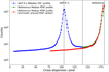 |
Fig. 1 Median PSF profiles of the target and the reference star from the R150 data. The B600 observations look similar. We have mirrored the reference star PSF profile around its peak (green and red) in order to illustrate our method of correcting for diluted light. The black line indicates the point where we separate the two spectra. Because we have ensured that the single-star PSFs observed with GMOS are symmetric, we can use the mirrored part of the PSF to estimate the amount of contamination on the target PSF. We also correct the reference star for diluted light from the target in a similar way. We extrapolate the red curve linearly for regions beyond the spatial range of the observation. The boundary (black line) we select between the target and reference stars was fixed as a function of time, although the spectral trace evolves withairmass and gravity vector on the instrument. However, this can be arbitrary (as long as it is reasonable) because the exact location of the boundary does not affect the amount of scattered light from the reference diluting the target flux extracted from the core of the target PSF. This is measured only using the opposite wing of the reference PSF, which is not affected by our choice of border. |
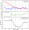 |
Fig. 2 Top: wind velocity and direction during the B600 transit observation, with respect to the current pointing vector of the telescope. The transverse wind component (red) comes from the right when positive and from the left when negative in the observer reference frame because it follows the target star during the night. The head-on wind component (blue) comes from the observer’s back when negative and from the front when positive. The transverse wind component coming from the right drops to zero near phase of 0.987 and then again increases in strength, but from the other direction. The head-on component of the wind remains fairly constant throughout the observation with respect to the dome opening, and always returns from the back of the observer. Middle: median PSF FWHM for each exposure throughout the observation, showing a spike of a factor of ~ 2 near phase 0.987, which coincides with the change in direction in the transverse wind component. The overall gradual increase in the FWHM beyond this point is likely caused by worsening seeing caused by the increasing airmass of the observation. Bottom: B600 white-light curve (black solid line) and a sketch of the ramp we use to correct the overall slopes. The green dotted vertical lines represent the two defects in the light curve that appear to cause changes in the baseline slope. The defect near 0.987 is likely induced by the change in the wind direction, while the cause of the other remains unclear. |
3.1.3 Ghost spectra
During both transit observations (B600 and R150), each spectral trace image was accompanied by a fainter trace-like signal. The amplitude of the signal is small, ~50 ppm, compared to the amplitude of the observed stellar spectrum. For both the reference and the targets stars, it was confined to between 22 and 30 pixels from the peak of the main trace, and followed the same spatial behavior as the main trace in all wavelengths. Despite its low amplitude, this spurious signal is clearly detected due to the extremely high signal-to-noise ratio of the median-combined spectral image of the HAT-P-1 stellar system over the entire night. However, attempting to extract its spectrum is difficult because it is dominated by the wings of the PSF of the main spectral trace. Thus, we cannot explore its spectral signature in detail, but its persistent appearance in the same location in all images and above both the target and reference stars suggests that it is likely caused by internal reflections within the instrument. Because it is highly localized, we masked the strip of pixels that showed this spurious signal and did not use them in our analysis.
3.2 Effect of terrestrial wind on the time series
The B600 white-light curve exhibits several unusual artifacts that could not be corrected or correlated with any of the methods that are frequently discussed in the literature. We explored the headers of the raw fits file and discovered that one of these artifacts (near phase 0.987) coincides with a sudden change in the transverse wind at the observatory site: the projected wind component, perpendicular to the line of sight of the telescope, switches direction from the right to the left (Fig. 2). We suggest that the abrupt change in the apparent baseline slope of the B600 white-light curve near phase 0.987 could be due to structural vibrations caused by the change in wind direction with respect to the line of sight, which affect the spectral PSF width. The timing of this defect is unfortunate because it coincides with the ingress of the transit. We removed these data from our analysis.
The leading one hour of the R150 white-light curve ends with a kink near phase 0.9805. At about this time, the direction of the head-on component of the wind from changes. It comes from the front instead of the back, as before. In this data set, the transverse component of the wind always comes from the left of the observer and is approximately constant. This change in the wind does not produce a corresponding spike in the spectral PSF full width at half-maximum (FWHM), as in the B600 observation, and we cannot unambiguously attribute the kink to it.
3.3 Wavelength calibration
After spectral extraction, we obtained the wavelength solution using CuAr lamp spectra taken on the same day as each science observation. To observe the CuAr spectra at high resolution, we used a separate MOS slit mask to that used for science, with the same slit position and slit length as the science mask, but the slit width was only 1′′ (compared to 10′′). The arc frames were obtained with the same grating and filter setup as the corresponding science observation.
We used the identify task in the Gemini IRAF package to identify the spectral features in the CuAr spectra. A wavelength solution wasthen constructed by fitting a straight line to the pixel locations of the spectral features and their known wavelengths. This solution was then refined by cross-correlating all spectra with the pixel locations of several known stellar and telluric features.
The final uncertainties in the wavelength solution are approximately 1 nm for all observations, which is ~ 3% and ~ 6− 7% of the bin widths used in the final transmission spectrum for the R150 and B600 transits, respectively. This level of uncertainty in the wavelength solution has been shown to be sufficient to avoid systematic effects caused by wavelength-dependent differences in the limb-darkening models we used to fit the transits in Sect. 4 (Huitson et al. 2017), and in addition, it is also smaller than our resolution element (~ 4 nm in R150 and ~2 nm in B600).
3.4 Dispersion-direction shifts of the stellar spectra
Because GMOS has no atmospheric dispersion compensator, we expect the wavelength solution to shift with time. Huitson et al. (2017) reported that throughout the night, individual spectra are shifted and stretched in the dispersion direction. The shift and stretch are both time and wavelength dependent. Left uncorrected for, this effect could introduce spurious signals in the observed transit spectrum of the planet. In order to avoid these systematic effects in the final light curves related to shifting wavelength solution with time, we applied a correction for this effect.
A priori differential refraction calculations alone do not explain the observed shifts for our observations well. Therefore we applied a cross-correlation to four spectral segments as a function of time to measure the spectral shift and stretch empirically, similarly to Huitson et al. (2017).
Finally, we corrected for the differential offset in wavelength between the reference and target star spectra on the detector. This offset is caused by the fact that the PA of the detector slit is slightly different from the PA of the reference star. We used a cross-correlation to measure the offset (1.57–1.63 pixels for all observations). We interpolated the reference star’s spectrum onto the target star’s wavelength solution. Bad columns (which are the same columns on the detector but are at different wavelengths for each star) were omitted.
We tested the effect of wavelength shifts with time by running our analysis with and without the correction. We find that for the low-resolution broad bins that we adopted, the correction results in differences typically smaller than 0.1 σ in both B600 and R150. However, the shift correction has a small effect on the narrow bins we used to investigate the Na absorption region. Therefore we chose to keep this correction in our analysis.
4 Transit light-curve analysis
We describe our transit depth measurements for the B600 and R150 observations below. First, we describe the model we used to correct for the systematic effects in Sect. 4.1. In Sect. 4.2 we focus on the wavelength-integrated white-light curves for each of the observations. Section 4.3 focuses on the transit light curves in individual wavelength bins, while Sect. 4.4 discusses the time series near the 589 nm Na I resonant doublet expected in the planet’s atmosphere. Section 4.5 addresses any potential variability in the host star based on the LCO data.
4.1 Light-curve model of systematic effects
To describe the systematic effects (telluric absorption and instrumental effects) in our light curves, we adopted the parameterization of Stevenson et al. (2014), who used the same instrument, GMOS, to study the transmission spectrum of the hot Jupiter WASP-12b in the red-optical. This model addresses effects caused by the Cassegrain Rotator Position Angle (CRPA), the airmass, and the time-varying PSF of the instrument. Our light-curve model also accounts for any approximately linear or quadratic trends as a function of time that are commonly seen in transit studies. We applied this model to both the R150 and B600 data and to both the white-light curves and the wavelength-dependent light curves.
We parameterized the systematic effect due to the CRPA by approximating the photometric dependence of the flux on the CRPA as a cosine function:
 (1)
(1)
Here, ACRPA and θCRPA are the free parameters, while θ(t) is the known CRPA as a function of time. Like Stevenson et al. (2014), we considered a systematic trend, or a “ramp”, as a function of time in the light curve in the form,
 (2)
(2)
where a and b are free parameters, while t is time and t0 is the time of observation of the first frame in the time series. However, we find that with our data, aramp is degenerate with the transit depth, and based on the resulting Bayesian information criterion (BIC) values, the data are better described by a pure linear ramp. We included an airmass correction:
 (3)
(3)
where α(t) is the known run of airmasses at the time of observation, and Cα is a free parameter.
These parameters account well for the long-timescale (hours) variations of the light curves, but do not correct short-timescale (≲ 10 min) effects. To address these, we experimented with several time-varying quantities: the ratio of the widths of the target and reference PSFs, the cross-dispersion position of the target PSF on the detector, and the dispersion direction shifts of the target spectrum. We find that most of these are correlated with the light curves at some level, but the data are best described by the width of the target PSF as a function of time:
 (4)
(4)
where CPSF width is a free parameter, and W(t) is the run of the median PSF widths throughout the observations. This correction term is likely related to the state of the atmosphere above the telescope during the observations.
Thus, the final model to fit to the light curve (normalized to the out-of-transit flux) can be represented as
 (5)
(5)
T(t) is the astrophysical transit light-curve model, normalized to 1 out-of-transit.
We used several open-source packages to model and fit the transit light curves. T(t) was calculated with the transit code batman (Kreidberg 2015), and for the fit we used emcee, a pure-Python implementation of the affine-invariant Markov chain Monte Carlo (MCMC) ensemble sampler (Goodman & Weare 2010; Foreman-Mackey et al. 2013). The stellar limb darkening was pre-computed for each wavelength bin using PyLDTk (Parviainen & Aigrain 2015), which uses the spectral library in Husser et al. (2013), based on the atmospheric code PHOENIX. We used the nonlinear parameterization for limb-darkening coefficients (Claret 2000; Sing 2010).
4.2 White-light curve
We constructed transit white-light curves for each transit (B600 and R150) by integrating each observed target and reference spectrum over wavelength and dividing one by the other. This approach eliminates many of the light-curve artifacts caused by variations in Earth’s atmosphere. Because some transit parameters are not wavelength dependent (e.g., the ratio of semimajor axis to stellar radius, a∕R⋆, the central time of transit, T0, and the orbital period, P), we can use the precise white-light curves, which have a high signal-to-noise ratio, to measure them, rather than the noisier light curves at specific wavelengths.
The data cover wide wavelength ranges from the blue optical to the near-infrared. Our B600 light curve includes intensity measurements between 330 and 770 nm. Similarly, we integrated the R150 spectral time series between 550 and 950 nm (Fig. 3). We estimated the uncertainties of each photometric point in two ways: from photon noise (assuming the only source of uncertainty of a given point is due to Poisson noise of the incoming photons), and based on the local scatterof the points, after subtracting a white-light curve smoothed by convolving it with a Gaussian. The latter approach is an empirical estimate of the uncertainty of the points, and we used it to fit the white-light curve.
As we discuss in Sect. 3.2, there is a sharp change in the slope of the ramp in the R150 data (Fig. 3), possibly related to a change in the head-on component of the wind. However, phase 0.9805 is also close to the phase where the target crossed the meridian (airmass of 1.057), and telescope field rotation may also have contributed. Regardless, the residuals of the first hour of observations (Fig. 3, bottom panel) show a different slope than the rest of the observation. Because this happens well before egress, we simplified our analysis and dropped these data. The final 45 min of R150 data were also excluded because they were taken at high airmass and their residuals are higher than those of the preceding white-light curve points.
We also removed the data near phase 0.987 in the B600 data set, where the light curve is strongly distorted. We removed all phases covered by the unusual spike in the PSF FWHM, which coincides with a change in the direction from which the transverse wind component impacts the dome (Fig. 2). We also dropped the last several minutes of this light curve, taken at high airmass where the white-light curve appears to become unstable (Fig. 3).
We fit the white-light curve with the model described in Sect. 4.1. In the statistical fits, we allowed the semimajor axis (a∕R⋆), the transit depth (Rp ∕R⋆), and the central time of transit (T0), which are a part of the T(t) calculation, to vary freely. A large uncertainty in the orbital inclination could result in a degeneracy with the slope of the transit spectrum (Alexoudi et al. 2018). However, the orbital parameters of HAT-P-1b are well known (e.g., Nikolov et al. 2014), therefore wefixed the limb-darkening coefficients and inclination of the planetary orbit in our analysis (Table 3).
Unlike the R150 white-light curve, the B600 white-light curve is poorly described by a single linear ramp. The white-light curve appears to increase slightly until the defect near orbital phase 0.987, after which the ramp slope appears to decrease with a shallow slope during ingress and then sharply drop off near phase 0.994 (Fig. 2). We experimented with a segmented version of the linear ramp and found that the fit quality and the BIC are optimal for a ramp with three segments (before phase 0.987, between 0.987 and 0.994, and after 0.994),where each segment is linear with a free slope. We explored a number of different configurations for the break points and correction parameters for the white-light curve. We tried to fit the B600 white-light curve without anybreak points, and using the airmass function to correct for the changing slope. This led to a reduced χ2 of the fit of 1.9 and BIC = 650. Relying on a single break point improved these values, but the best fits were achieved with two break points: reduced χ2 = 0.94, and BIC = 360, showing a clear preference for the models with two break points. The location of the break near 0.994 is clearly visible by eye, while for the break near 0.987, we ran the white-light curve fit on a grid of locations and selected the location that yielded the best BIC. We experimented by letting the break-point locations vary as a free parameter, but the MCMC fits did not converge, even with strict priors. We therefore fixed the break-point locations. At these pointsthe adjacent segments of the ramp were required to have the same value to avoid discrete jumps in the ramp.
Additional detrending options can be explored (e.g., Stevenson et al. 2014), but regardless of that choice, the ramp slope of this observation is variable and changes sharply during ingress and the transit itself. Because of this, any decorrelation function that could be applied to the B600 data would be degenerate with the transit depth, leading to larger transit spectrum uncertainties (Sect. 4.3).
We present the R150 white-light curve corrected for systematic effects in Fig. 4 and compare it to an HST/STIS white-light curves in the optical (Nikolov et al. 2014). In our fit, we kept the inclination of the system fixed to the value found by Nikolov et al. (2014), based on multiple HST transits with the STIS and WFC3 instruments. The a∕R⋆ parameter we find for the R150 light curve is well within 1 σ of the HST value.
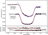 |
Fig. 3 White-light curves of the transits observed with the B600 and R150 grating spectral time series integrated over wavelength between 330 and 770 nm and 550 and 950 nm, respectively. Gray points indicate poor-quality data excluded from the analysis. The anomalous peak near phase 0.987 in the B600 light curve has an amplitude of about 0.5% and represents a defect in the light curve, likely caused by rapid change in the wind at the observatory site, correlated with a spike in the PSF FWHM (Fig. 2). Near phase 0.987, we exclude the part of the spectral time series with anomalously broad PSFs. The R150 light curve appears to be better behaved and displays no large-scale irregularities, but the initial hour of the light curve is difficult to account for with our model of systematic effects. We drop it from the analysis, along with the final ~ 45 min, which were obtained at high airmass and have a large scatter. The red lines represent the best-fit model of the transit and systematic effects for the white-light curve (top) and the smoothed residuals to highlight any residual red noise (bottom). The faint blue lines in the top panel represent sample model instances from the converged MCMC chains. |
Best-fit parameters for the white-light curve MCMC.
4.3 Transit spectrum
We divided the time-series spectra into wavelength bins. For consistency, we used 200 pixel bins in both R150 and B600, which corresponds to bins of 36 and 16 nm, respectively. To measure the transit spectrum of HAT-P-1b, we applied the model discussed in the previous section to the transit light curves corresponding to individual wavelength bins (λLC) with several changes. To correct for wavelength-independent systematic effects that were not accounted for by our white-light curve model, we divided eachλLC by the white-light curve residuals (data minus best-fit model). We smoothed the white-light curve residuals byconvolving them with a Gaussian to reduce the effect of high-frequency noise when the light curve was divided. When we skipped this step, the point-to-point scatter in the R150 and B600 λLCs typically increased by~20 and ≲ 5%, respectively. This common-mode correction resulted in lower χ2 fits, but did not constitute an additional free parameter because we always divided the light curves by the same white-light curve residuals.
We fixed the ratio of the semimajor axis to stellar radius, a∕R⋆, the central time of transit, T0 to their best-fit values from the white-light curve fits because they are wavelength independent. The transit depth, ACRPA, θCRPA, Cα, and CPSF width remained free, as were the linear ramp parameters. As with the white-light curve, we used a segmented ramp for the B600 λLCs.
We fit each light curve in every bin again using the PyLDTk code to compute the limb-darkening coefficients and the emcee package to retrieve the posterior distributions of the wavelength-dependent free parameters. We plot the transit fit results in Figs. 5 and 6. While the typical R150 light curve appears to be well corrected for systematic effects, the fits near 750 and ≳ 850 nm are potentially unreliable due additional correlated noise effects of strong and variable telluric absorption by O2 and H2 O, respectively. The B600 data at wavelengths shorter than ~400 nm are heavily affected by high airmass toward the end of the observation. We tabulate both the R150 and B600 transit spectra in Table 4.
The uncertainties of photometric points in each light curve were estimated as described in Sect. 4.2. We estimated how well our data corrections work by comparing uncertainties in Rp ∕R⋆ for the fits where we assumed pure photon noise for the points in the light curves to the fits using the empirical photometric scatter (Table 4).
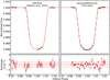 |
Fig. 4 Comparison of the GMOS R150 transit white-light curve (right panels, 4σ outliers removed) after correction for systematic effects to a corrected HST/STIS optical white-light curve (left panels, Nikolov et al. 2014). The HST transit was observed on 2012 May 30 (Visit 20) with the G750L grating (524– 1027 nm). The GMOS R150 white-light curve is binned to match the HST integration time (284 s). In the white-light curves, the scatter of the residuals is comparable between the two instruments. The rms of the residuals (dashed lines) is 90 ppm (HST/STIS) and 100 ppm (Gemini/GMOS), but GMOS can observe the transit continuously, while HST observations have gaps because the spacecraft orbits Earth. While the R150 observation is comparable in precision to that with HST/STIS, the B600 observation (not shown) is subject to more complex systematic effects and the corresponding rms of the residuals and the uncertainties in the transit parameters is higher than for space-based observationsat similar wavelengths. |
4.4 Core of the Na I absorption line
Both the R150 and the B600 spectra cover the Na I doublet at 589 nm. Sodium has been detected in the atmosphere of HAT-P-1b by Nikolov et al. (2014) and Sing et al. (2016) in the narrow core of the line (3 nm wide bin centered on 589.3 nm at 3.3σ). However, these authors did not detect the pressure-broadened wings of the Na feature.
We explored this wavelength region by comparing the narrow-band transit depth in the core of the sodium line in both the R150 and B600 observations with the broadband transit depth in that region. We divided the region around the Na I line into narrow-band bins of 2 nm each. The bins overlap each other by 1 nm in order to ensure that any increase in measured Rp ∕R⋆ is not due to asingle anomalous pixel or pixel column. The overlapping-bin light curves were fit as described in Sect. 4.3.
If the feature is real, it should ideally result in a smooth rise and drop of transit depths as a function of wavelength, essentially tracing the dispersion function of the instrument. This approach does not rule out wavelength-dependent systematic effects, but prevents our results from being influenced by a spurious feature due to a pixel defect that might produce a sharp and discontinuous change in transit depth. We tested this on wavelengths beyond the immediate vicinity of the Na I feature where we expect the spectrum to be flat. Seeing features in our spectrum in this region might indicate that narrow-band transit depth variations are difficult to measure reliably with Gemini/GMOS. In addition, we experimented with the “divide white” approach described by Stevenson et al. (2014), for example, where we compared the transit depth in the narrow-wavelength region around the Na I line to a transit light curve covering a wider wavelength region around the feature. For both transit observations, these two approaches result in narrow-band spectra that are consistent with flat lines, and we did not detect narrow-band Na absorption. Scaling our narrow-band uncertainties to the bin size of Nikolov et al. (2014), we expect that their 3.3σ Na I narrow-band absorption detection would translate into a 2.1σ detection in our R150 observation, which is marginal, and therefore we did not consider our nondetection to be in disagreement with the HST study.
Another aspect of our observations is that they are seeing limited (~ 1.5′′), corresponding to a resolution element (line-spread function width) of ~ 3.5 nm near a wavelength of 600 nm. This is similar to the bin size used by Nikolov et al. (2014) and also Nikolov et al. (2016, 3 nm bin centered on 589 nm), for instance, who observed the core of the Na line on the warm Saturn-mass exoplanet WASP-39b using ground-based transit spectroscopy with the FOcal Reducer/low dispersion Spectrograph 2 (FORS2) instrument on the Very Large Telescope (VLT).
Both observations in principle also cover the K I resonant doublet at 770 nm. This wavelength is strongly affected by telluric O2 absorption, however, and our systematic corrections are not reliable. We therefore excluded these data from consideration.
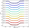 |
Fig. 5 R150 light curves in each wavelength bins (labeled) and the best-fit transit models (black lines). We indicate the rms values of the residuals between observation and model in order to quantify the scatter in each wavelength bin. |
4.5 Stellar variability
Star spots and surface inhomogeneities have been known to affect the apparent transit depth at a given wavelength, potentially affecting thetransit spectrum of a transiting exoplanet. Star spots occulted by the planet during transit have been investigated in detail (e.g., Désert et al. 2011a,b; Nutzman et al. 2011; Sanchis-Ojeda et al. 2011). We see no evidence of star spot occultations during transit in either of our white-light curves. More recently, McCullough et al. (2014) and Rackham et al. (2017), for example, have shown that unocculted star spots can mimic a Rayleigh-like slope in the transit spectra of exoplanets due to what the latter authors called the transit light-source effect (TLSE). Faculae have been demonstrated to potentially affect the transit depths near strong stellar absorption lines such as Hα, Ca II K, and Na I D (e.g., Cauley et al. 2018; Rackham et al. 2019). Espinoza et al. (2019) analyzed six transit spectroscopy observations of the hot Jupiter WASP-19b and characterized the surface of the host star. They detected two spot-crossing events, including a planetary occultation of a bright spot.
However, HAT-P-1 and its companion (which is our reference star) have not been reported to show signs of activity so far. Bakos et al. (2007) reported low atmospheric variability for both stars. Measurements of the Ca II H&K activity index of HAT-P-1,  have yielded a value of − 4.984, which indicates relatively low activity (Noyes et al. 1984; Knutson et al. 2010). Nikolov et al. (2014) monitored HAT-P-1 for 223 days, between 2012 May 4 and 2012 December 13, using the RISE camera on the Liverpool Telescope. This campaign covers our R150 observation on November 12, and Nikolov et al. (2014) placed an upper limit on the variability of the star of 0.5%.
We also examined the potential for variability and activity of the host star. We used our LCO photometric monitoring in the Johnson-Cousins/Bessell B-band, which should be particularly sensitive to magnetic star spots. Even though our photometric monitoring covers eight months in 2016 (Sect. 2.2) and does not cover our transit observations, any detection of variability in the B band would indicate that star spots and the TLSE effect need to be taken into account. We removed the photometric points taken during transit and secondary eclipse (20 and 37 points, respectively). We created a Lomb-Scargle periodogram using the remaining 617 data points in order to identify the stellar rotation period and the amplitude of variability, thus estimating the fraction of the stellar surface covered by spots (Fig. 7). However, we find no peak in the periodogram near the expected stellar rotation period (≲ 15 days, based on rotational line broadening, Johnson et al. 2008). This suggests that the star had few if any stellar spots during the period it was monitored. We find no evidence for stellar activity in our photometric and spectroscopic data, nor in the literature. We therefore do not consider it necessary to correct our results for the transit light-source effect.
Our periodogram in Fig. 7 suggests a tentative low-amplitude periodic variation (0.5% in the B band, consistent with Nikolov et al. 2014) that coincides with the planetary orbital period. It is unlikely that this signal is an alias of the stellar rotation period because we do not detect its primary order. We speculate that this variability might be an indication of a magnetic planet–star interaction, although in this case, the variability period would be expected to be the synodic period of the star in the frame of the planet (≲ 6.3 days, see, e.g., Fischer & Saur 2019).
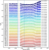 |
Fig. 6 Similar to Fig. 5, but for the B600 data. We denote our transit model break points with vertical blue lines. |
HAT-P-1b transit spectrum.
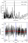 |
Fig. 7 Panel a: Lomb-Scargle periodogram of our LCO B-band long-term photometric monitoring of HAT-P-1b (in-transit and in-eclipse measurements excluded). The only interesting peak in the periodogram, near 4.4866 days, with an FAP of ~ 4 ppm, corresponds to the orbital period of the planet. The other significant peak, near 1.3 days, is likely an alias of the LCO photometriccadence (typically one measurement every eight hours). The rotation period of the star is expected to be ≲ 15 days. Panel b: our stellar photometry folded to the period of the planet (4.465 days) and fit with a sine curve. Red squares represent the photometry binned to ~ 11 h (0.1 of the orbital period of the planet). The variation (minimum to maximum) is about 0.5%, which is smaller than the transit depth. It varies slowly and therefore probably does not affect our transit spectrum measurements. The timings of the transit and the secondary eclipse are marked. |
5 Discussion
We compareour observed transit spectrum to models computed using the Exo-Transmit code (Kempton et al. 2016) and to previous studies. The uncertainties of the spectrophotometry in the B600 observations exceed the photon noise by a factor of up to four. This is likely an effect of the complex systematic effects that influence this data set, compounded by the high airmass toward the end of the transit observation. Consequently, the resulting B600 transit spectrum is consistent with both cloudy and clear models, and does not have the necessary precision to constrain the transit spectrum of HAT-P-1b. Because the effect of the airmass on the data quality is especially strong at wavelengths ≲ 500 nm, it is difficultto place limits on the Rayleigh slope in the atmosphere of HAT-P-1b based on these data.
The R150 observation is less affected by systematic effects and typical uncertainties are only ~ 50% above photon noise. The transit depths measured in R150 are comparable in terms of precision to the measurements made with HST/STIS, and the two observations are consistent with each other (Fig. 8).
We compared the R150 reduced-χ2 values for several exo-transmit models (Table 5). All models we considered have isothermal atmospheres at 1500 K, which is close to the equilibrium temperature of the planet. Our spectrum excludes strong TiO and VO features and shows preference to models with cloud decks deep in the atmosphere, or completely clear atmospheres. This is consistent with the HST/STIS results in Nikolov et al. (2014) and Sing et al. (2016), and also with ground-based broadband transit measurements with TNG/DOLORES (Montalto et al. 2015). Atmospheric spectra without clear TiO and VO absorption features are common in hot Jupiters with equilibrium temperatures similar to that of HAT-P-1b (e.g., Désert et al. 2008; Sing et al. 2016).
We tested whether our observations can be used to probe narrow-band features like the Na I resonance doublet at 589 nm. Unlike Nikolov et al. (2014), we did not detect the core of the Na absorption line, but our uncertainty estimates on the narrow-band transit depth uncertainties are ~60% larger than those derived from the HST observations, which might explain this difference. We did not observe the broad line wings either, but this is consistent with the results of Nikolov et al. (2014), who also did not detect them.
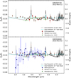 |
Fig. 8 R150 (top) and B600 (bottom) transit spectra from this work, compared to the results of Nikolov et al. (2014) and Montalto et al. (2015). The bluest wavelengths in the B600 spectrum are strongly affected by high airmass, and this spectrum as a whole has little constraining power on atmospheric models. The R150 measurements near 750 nm and ≳ 850 nm could be affected by additional correlated noise effects of strong and variable telluric absorption by O2 and H2O, respectively. We therefore exclude these transit measurements from our analysis and this figure. We compare the resulting transit spectrum to an exo-transmit model with clear atmosphere and no TiO/VO (black lines), which, based on our observations, is marginally favored over cloudy models, which are essentially flat lines (cyan lines). The model that does not include gas condensation and contains TiO/VO (not shown for clarity) is marginally disfavored by the R150 data. The R150 measurements have comparable uncertainties to the HST/STIS measurements (brown squares) for wavelength bin sizes of of tens of nanometers. |
R150 model results.
6 Conclusion
We presented ground-based observations of the visible low-resolution transit spectrum of the hot Jupiter HAT-P-1b. We showed that transit spectroscopy observations from the ground can be comparable to HST/STIS in precision and in information content, as is the case of our R150 observation. Based on our R150 observations between 550 and 850 nm, we are able to reject models with a high abundance of TiO and VO. This is consistent with the findings of previous space-based studies with HST/STIS. The B600 transit data are affected by strong systematic effects and result in a highly uncertain transit spectrum.
Our long-term photometric B-band monitoring of the host star, HAT-P-1, suggests that its activity is very low and is unlikely to affect our spectrophotometry. However, our Lomb-Scargle diagram results in an unexpected peak at the planetary orbital period. Because of this, we speculate that planet–star interactions might play a role in this system.
Acknowledgements
We thank the referee for a careful and balanced review. We thank Jacob Arcangeli, Claire Baxter, and Gabriela Muro-Arena for useful discussions, and Nikolay Nikolov for graciously sharing with us the HST/STIS white light curves. This work isbased on observations obtained at the Gemini Observatory (acquired through the Gemini Observatory Archive and Gemini Science Archive), which is operated by the Association of Universities for Research in Astronomy, Inc. (AURA), under a cooperative agreement with the NSF on behalf of the Gemini partnership: the National Science Foundation (United States), the National Research Council (Canada), CONICYT (Chile), Ministerio de Ciencia, Tecnología e Innovación Productiva (Argentina), and Ministério da Ciência, Tecnologia e Inovação (Brazil). Based in part on Gemini observationsobtained from the National Optical Astronomy Observatory (NOAO) Prop. ID: 2012B-0398; PI: J.-M. Désert. This work makes use of observations from the LCOGT network. J.M.D acknowledges support by the Amsterdam Academic Alliance (AAA) Program. The research leading to these results has received funding from the European Research Council (ERC) under the European Union’s Horizon 2020 research and innovation programme (grant agreement no. 679633; Exo-Atmos). This material is based upon work supported by the National Science Foundation (NSF) under Grant No. AST-1413663, and supported by the NWO TOP Grant Module 2 (Project Number 614.001.601). This research has made use of NASA’s Astrophysics Data System. This research made use of Astropy (http://www.astropy.org), a community-developed core Python package for Astronomy (Astropy Collaboration 2013, 2018). Other software used: diff_atm_refr.pro (http://www.eso.org/gen-fac/pubs/astclim/lasilla/diffrefr.html); ATLAS (Kurucz 1993, available at http://kurucz.harvard.edu); MPFIT (Markwardt 2009); Time Utilities (Eastman et al. 2010).
References
- Alexoudi, X., Mallonn, M., von Essen, C., et al. 2018, A&A, 620, A142 [NASA ADS] [CrossRef] [EDP Sciences] [Google Scholar]
- Arcangeli, J., Désert, J.-M., Line, M. R., et al. 2018, ApJ, 855, L30 [NASA ADS] [CrossRef] [Google Scholar]
- Astropy Collaboration (Robitaille, T. P., et al.) 2013, A&A, 558, A33 [NASA ADS] [CrossRef] [EDP Sciences] [Google Scholar]
- Astropy Collaboration (Price-Whelan, A. M., et al.) 2018, AJ, 156, 123 [Google Scholar]
- Bakos, G. Á., Noyes, R. W., Kovács, G., et al. 2007, ApJ, 656, 552 [NASA ADS] [CrossRef] [Google Scholar]
- Bean, J. L., Miller-Ricci Kempton, E., & Homeier, D. 2010, Nature, 468, 669 [NASA ADS] [CrossRef] [PubMed] [Google Scholar]
- Bean, J. L., Désert, J.-M., Kabath, P., et al. 2011, ApJ, 743, 92 [NASA ADS] [CrossRef] [Google Scholar]
- Bixel, A., Rackham, B. V., Apai, D., et al. 2019, AJ, 157, 68 [NASA ADS] [CrossRef] [Google Scholar]
- Bouma, L. G., Winn, J. N., Baxter, C., et al. 2019, AJ, 157, 217 [NASA ADS] [CrossRef] [Google Scholar]
- Brown, T. M., Baliber, N., Bianco, F. B., et al. 2013, PASP, 125, 1031 [NASA ADS] [CrossRef] [Google Scholar]
- Cauley, P. W., Kuckein, C., Redfield, S., et al. 2018, AJ, 156, 189 [Google Scholar]
- Charbonneau, D., Brown, T. M., Noyes, R. W., & Gilliland, R. L. 2002, ApJ, 568, 377 [NASA ADS] [CrossRef] [Google Scholar]
- Claret, A. 2000, A&A, 363, 1081 [NASA ADS] [Google Scholar]
- de Mooij, E. J. W., de Kok, R. J., Nefs, S. V., & Snellen, I. A. G. 2011, A&A, 528, A49 [NASA ADS] [CrossRef] [EDP Sciences] [Google Scholar]
- Deming, D., Wilkins, A., McCullough, P., et al. 2013, ApJ, 774, 95 [NASA ADS] [CrossRef] [Google Scholar]
- Désert, J. M., Vidal-Madjar, A., Lecavelier Des Etangs, A., et al. 2008, A&A, 492, 585 [NASA ADS] [CrossRef] [EDP Sciences] [Google Scholar]
- Désert, J.-M., Charbonneau, D., Demory, B.-O., et al. 2011a, ApJS, 197, 14 [NASA ADS] [CrossRef] [Google Scholar]
- Désert, J. M., Sing, D., Vidal-Madjar, A., et al. 2011b, A&A, 526, A12 [NASA ADS] [CrossRef] [EDP Sciences] [Google Scholar]
- Eastman, J., Siverd, R., & Gaudi, B. S. 2010, PASP, 122, 935 [NASA ADS] [CrossRef] [Google Scholar]
- Espinoza, N., Rackham, B. V., Jordán, A., et al. 2019, MNRAS, 482, 2065 [Google Scholar]
- Fischer, C., & Saur, J. 2019, ApJ, 872, 113 [NASA ADS] [CrossRef] [Google Scholar]
- Foreman-Mackey, D., Hogg, D. W., Lang, D., & Goodman, J. 2013, PASP, 125, 306 [CrossRef] [Google Scholar]
- Gibson, N. P., Aigrain, S., Barstow, J. K., et al. 2013a, MNRAS, 428, 3680 [NASA ADS] [CrossRef] [Google Scholar]
- Gibson, N. P., Aigrain, S., Barstow, J. K., et al. 2013b, MNRAS, 436, 2974 [NASA ADS] [CrossRef] [Google Scholar]
- Goodman, J., & Weare, J. 2010, Commun. Appl. Math. Comput. Sci., 5, 65 [Google Scholar]
- Høg, E., Fabricius, C., Makarov, V. V., et al. 2000, A&A, 355, L27 [Google Scholar]
- Hook, I. M., Jørgensen, I., Allington-Smith, J. R., et al. 2004, PASP, 116, 425 [NASA ADS] [CrossRef] [Google Scholar]
- Horne, K. 1986, PASP, 98, 609 [NASA ADS] [CrossRef] [EDP Sciences] [Google Scholar]
- Huitson, C. M., Désert, J.-M., Bean, J. L., et al. 2017, AJ, 154, 95 [NASA ADS] [CrossRef] [Google Scholar]
- Husser, T.-O., Wende-von Berg, S., Dreizler, S., et al. 2013, A&A, 553, A6 [NASA ADS] [CrossRef] [EDP Sciences] [Google Scholar]
- Johnson, J. A., Winn, J. N., Narita, N., et al. 2008, ApJ, 686, 649 [NASA ADS] [CrossRef] [Google Scholar]
- Kempton, E. M.-R., Lupu, R. E., Owusu-Asare, A., Slough, P., & Cale, B. 2016, Astrophysics Source Code Library [record ascl:1611.005] [Google Scholar]
- Knutson, H. A., Howard, A. W., & Isaacson, H. 2010, ApJ, 720, 1569 [NASA ADS] [CrossRef] [Google Scholar]
- Kreidberg, L. 2015, PASP, 127, 1161 [NASA ADS] [CrossRef] [Google Scholar]
- Kurucz, R. 1993, ATLAS9 Stellar Atmosphere Programs and 2 km/s grid. Kurucz CD-ROM No. 13 (Cambridge, MA: Smithsonian Astrophysical Observatory), 13 [Google Scholar]
- Markwardt, C. B. 2009, ASP Conf. Ser., 411, 251 [Google Scholar]
- McCullough, P. R., Crouzet, N., Deming, D., & Madhusudhan, N. 2014, ApJ, 791, 55 [NASA ADS] [CrossRef] [Google Scholar]
- Montalto, M., Iro, N., Santos, N. C., et al. 2015, ApJ, 811, 55 [NASA ADS] [CrossRef] [Google Scholar]
- Murgas, F., Pallé, E., Zapatero Osorio, M. R., et al. 2014, A&A, 563, A41 [NASA ADS] [CrossRef] [EDP Sciences] [Google Scholar]
- Murgas, F., Chen, G., Pallé, E., Nortmann, L., & Nowak, G. 2019, A&A, 622, A172 [NASA ADS] [CrossRef] [EDP Sciences] [Google Scholar]
- Nikolov, N., Sing, D. K., Pont, F., et al. 2014, MNRAS, 437, 46 [NASA ADS] [CrossRef] [Google Scholar]
- Nikolov, N., Sing, D. K., Gibson, N. P., et al. 2016, ApJ, 832, 191 [NASA ADS] [CrossRef] [Google Scholar]
- Nortmann, L., Pallé, E., Murgas, F., et al. 2016, A&A, 594, A65 [NASA ADS] [CrossRef] [EDP Sciences] [Google Scholar]
- Nortmann, L., Pallé, E., Salz, M., et al. 2018, Science, 362, 1388 [NASA ADS] [CrossRef] [EDP Sciences] [Google Scholar]
- Noyes, R. W., Hartmann, L. W., Baliunas, S. L., Duncan, D. K., & Vaughan, A. H. 1984, ApJ, 279, 763 [NASA ADS] [CrossRef] [Google Scholar]
- Nutzman, P. A., Fabrycky, D. C., & Fortney, J. J. 2011, ApJ, 740, L10 [NASA ADS] [CrossRef] [Google Scholar]
- Parviainen, H., & Aigrain, S. 2015, MNRAS, 453, 3821 [Google Scholar]
- Rackham, B., Espinoza, N., Apai, D., et al. 2017, ApJ, 834, 151 [NASA ADS] [CrossRef] [Google Scholar]
- Rackham, B. V., Apai, D., & Giampapa, M. S. 2019, AJ, 157, 96 [NASA ADS] [CrossRef] [Google Scholar]
- Redfield, S., Endl, M., Cochran, W. D., & Koesterke, L. 2008, ApJ, 673, L87 [NASA ADS] [CrossRef] [MathSciNet] [Google Scholar]
- Sánchez-Janssen, R., Mieske, S., Selman, F., et al. 2014, A&A, 566, A2 [NASA ADS] [CrossRef] [EDP Sciences] [Google Scholar]
- Sanchis-Ojeda, R., Winn, J. N., Holman, M. J., et al. 2011, ApJ, 733, 127 [NASA ADS] [CrossRef] [Google Scholar]
- Sing, D. K. 2010, A&A, 510, A21 [Google Scholar]
- Sing, D. K., Huitson, C. M., Lopez-Morales, M., et al. 2012, MNRAS, 426, 1663 [NASA ADS] [CrossRef] [Google Scholar]
- Sing, D. K., Fortney, J. J., Nikolov, N., et al. 2016, Nature, 529, 59 [NASA ADS] [CrossRef] [Google Scholar]
- Snellen, I. A. G., Albrecht, S., de Mooij, E. J. W., & Le Poole, R. S. 2008, A&A, 487, 357 [NASA ADS] [CrossRef] [EDP Sciences] [Google Scholar]
- Stevenson, K. B., Bean, J. L., Seifahrt, A., et al. 2014, AJ, 147, 161 [NASA ADS] [CrossRef] [Google Scholar]
- Todorov, K., Deming, D., Harrington, J., et al. 2010, ApJ, 708, 498 [NASA ADS] [CrossRef] [Google Scholar]
- Vidal-Madjar, A., Lecavelier des Etangs, A., Désert, J. M., et al. 2003, Nature, 422, 143 [NASA ADS] [CrossRef] [PubMed] [Google Scholar]
- von Essen, C., Cellone, S., Mallonn, M., et al. 2017, A&A, 603, A20 [NASA ADS] [CrossRef] [EDP Sciences] [Google Scholar]
- Wakeford, H. R., Sing, D. K., Deming, D., et al. 2013, MNRAS, 435, 3481 [NASA ADS] [CrossRef] [Google Scholar]
- Wilson, P. A., Sing, D. K., Nikolov, N., et al. 2015, MNRAS, 450, 192 [NASA ADS] [CrossRef] [Google Scholar]
- Zacharias, N., Finch, C. T., Girard, T. M., et al. 2013, AJ, 145, 44 [NASA ADS] [CrossRef] [EDP Sciences] [Google Scholar]
All Tables
All Figures
|
Fig. 1 Median PSF profiles of the target and the reference star from the R150 data. The B600 observations look similar. We have mirrored the reference star PSF profile around its peak (green and red) in order to illustrate our method of correcting for diluted light. The black line indicates the point where we separate the two spectra. Because we have ensured that the single-star PSFs observed with GMOS are symmetric, we can use the mirrored part of the PSF to estimate the amount of contamination on the target PSF. We also correct the reference star for diluted light from the target in a similar way. We extrapolate the red curve linearly for regions beyond the spatial range of the observation. The boundary (black line) we select between the target and reference stars was fixed as a function of time, although the spectral trace evolves withairmass and gravity vector on the instrument. However, this can be arbitrary (as long as it is reasonable) because the exact location of the boundary does not affect the amount of scattered light from the reference diluting the target flux extracted from the core of the target PSF. This is measured only using the opposite wing of the reference PSF, which is not affected by our choice of border. |
| In the text | |
|
Fig. 2 Top: wind velocity and direction during the B600 transit observation, with respect to the current pointing vector of the telescope. The transverse wind component (red) comes from the right when positive and from the left when negative in the observer reference frame because it follows the target star during the night. The head-on wind component (blue) comes from the observer’s back when negative and from the front when positive. The transverse wind component coming from the right drops to zero near phase of 0.987 and then again increases in strength, but from the other direction. The head-on component of the wind remains fairly constant throughout the observation with respect to the dome opening, and always returns from the back of the observer. Middle: median PSF FWHM for each exposure throughout the observation, showing a spike of a factor of ~ 2 near phase 0.987, which coincides with the change in direction in the transverse wind component. The overall gradual increase in the FWHM beyond this point is likely caused by worsening seeing caused by the increasing airmass of the observation. Bottom: B600 white-light curve (black solid line) and a sketch of the ramp we use to correct the overall slopes. The green dotted vertical lines represent the two defects in the light curve that appear to cause changes in the baseline slope. The defect near 0.987 is likely induced by the change in the wind direction, while the cause of the other remains unclear. |
| In the text | |
|
Fig. 3 White-light curves of the transits observed with the B600 and R150 grating spectral time series integrated over wavelength between 330 and 770 nm and 550 and 950 nm, respectively. Gray points indicate poor-quality data excluded from the analysis. The anomalous peak near phase 0.987 in the B600 light curve has an amplitude of about 0.5% and represents a defect in the light curve, likely caused by rapid change in the wind at the observatory site, correlated with a spike in the PSF FWHM (Fig. 2). Near phase 0.987, we exclude the part of the spectral time series with anomalously broad PSFs. The R150 light curve appears to be better behaved and displays no large-scale irregularities, but the initial hour of the light curve is difficult to account for with our model of systematic effects. We drop it from the analysis, along with the final ~ 45 min, which were obtained at high airmass and have a large scatter. The red lines represent the best-fit model of the transit and systematic effects for the white-light curve (top) and the smoothed residuals to highlight any residual red noise (bottom). The faint blue lines in the top panel represent sample model instances from the converged MCMC chains. |
| In the text | |
|
Fig. 4 Comparison of the GMOS R150 transit white-light curve (right panels, 4σ outliers removed) after correction for systematic effects to a corrected HST/STIS optical white-light curve (left panels, Nikolov et al. 2014). The HST transit was observed on 2012 May 30 (Visit 20) with the G750L grating (524– 1027 nm). The GMOS R150 white-light curve is binned to match the HST integration time (284 s). In the white-light curves, the scatter of the residuals is comparable between the two instruments. The rms of the residuals (dashed lines) is 90 ppm (HST/STIS) and 100 ppm (Gemini/GMOS), but GMOS can observe the transit continuously, while HST observations have gaps because the spacecraft orbits Earth. While the R150 observation is comparable in precision to that with HST/STIS, the B600 observation (not shown) is subject to more complex systematic effects and the corresponding rms of the residuals and the uncertainties in the transit parameters is higher than for space-based observationsat similar wavelengths. |
| In the text | |
|
Fig. 5 R150 light curves in each wavelength bins (labeled) and the best-fit transit models (black lines). We indicate the rms values of the residuals between observation and model in order to quantify the scatter in each wavelength bin. |
| In the text | |
|
Fig. 6 Similar to Fig. 5, but for the B600 data. We denote our transit model break points with vertical blue lines. |
| In the text | |
|
Fig. 7 Panel a: Lomb-Scargle periodogram of our LCO B-band long-term photometric monitoring of HAT-P-1b (in-transit and in-eclipse measurements excluded). The only interesting peak in the periodogram, near 4.4866 days, with an FAP of ~ 4 ppm, corresponds to the orbital period of the planet. The other significant peak, near 1.3 days, is likely an alias of the LCO photometriccadence (typically one measurement every eight hours). The rotation period of the star is expected to be ≲ 15 days. Panel b: our stellar photometry folded to the period of the planet (4.465 days) and fit with a sine curve. Red squares represent the photometry binned to ~ 11 h (0.1 of the orbital period of the planet). The variation (minimum to maximum) is about 0.5%, which is smaller than the transit depth. It varies slowly and therefore probably does not affect our transit spectrum measurements. The timings of the transit and the secondary eclipse are marked. |
| In the text | |
|
Fig. 8 R150 (top) and B600 (bottom) transit spectra from this work, compared to the results of Nikolov et al. (2014) and Montalto et al. (2015). The bluest wavelengths in the B600 spectrum are strongly affected by high airmass, and this spectrum as a whole has little constraining power on atmospheric models. The R150 measurements near 750 nm and ≳ 850 nm could be affected by additional correlated noise effects of strong and variable telluric absorption by O2 and H2O, respectively. We therefore exclude these transit measurements from our analysis and this figure. We compare the resulting transit spectrum to an exo-transmit model with clear atmosphere and no TiO/VO (black lines), which, based on our observations, is marginally favored over cloudy models, which are essentially flat lines (cyan lines). The model that does not include gas condensation and contains TiO/VO (not shown for clarity) is marginally disfavored by the R150 data. The R150 measurements have comparable uncertainties to the HST/STIS measurements (brown squares) for wavelength bin sizes of of tens of nanometers. |
| In the text | |
Current usage metrics show cumulative count of Article Views (full-text article views including HTML views, PDF and ePub downloads, according to the available data) and Abstracts Views on Vision4Press platform.
Data correspond to usage on the plateform after 2015. The current usage metrics is available 48-96 hours after online publication and is updated daily on week days.
Initial download of the metrics may take a while.