| Issue |
A&A
Volume 630, October 2019
|
|
|---|---|---|
| Article Number | A143 | |
| Number of page(s) | 14 | |
| Section | Interstellar and circumstellar matter | |
| DOI | https://doi.org/10.1051/0004-6361/201935883 | |
| Published online | 09 October 2019 | |
Interstellar dust along the line of sight of GX 3+1★
1
SRON Netherlands Institute for Space Research,
Sorbonnelaan 2, 3584 CA Utrecht, The Netherlands
e-mail: This email address is being protected from spambots. You need JavaScript enabled to view it.
2
Anton Pannekoek Astronomical Institute, University of Amsterdam,
PO Box 94249, 1090 GE Amsterdam, The Netherlands
3
Academia Sinica Institute of Astronomy and Astrophysics,
11F of AS/NTU Astronomy-Mathematics Building, No. 1, Section 4, Roosevelt Rd, Taipei 10617, Taiwan, PR China
4
Debye Institute for Nanomaterials Science, Utrecht University, Universiteitweg 99,
3584 CG Utrecht, The Netherlands
5
Astrophysikalisches Institut und Universitäts-Sternwarte (AIU),
Schillergäßchen 2-3, 07745 Jena, Germany
Received:
13
May
2019
Accepted:
30
August
2019
Abstract
Context. Studying absorption and scattering of X-ray radiation by interstellar dust grains allows us to access the physical and chemical properties of cosmic grains even in the densest regions of the Galaxy.
Aims. We aim at characterising the dust silicate population which presents clear absorption features in the energy band covered by the Chandra X-ray Observatory. Through these absorption features, in principle, it is possible to infer the size distribution, composition, and structure of silicate in the interstellar medium. In particular, in this work we investigate magnesium and silicon K-edges.
Methods. We built X-ray extinction models for 15 dust candidates using newly acquired synchrotron measurements. These models were adapted for astrophysical analysis and implemented in the SPEX spectral fitting program. We used the models to reproduce the dust absorption features observed in the spectrum of the bright low mass X-ray binary GX 3+1, which is used as a background source.
Results. With the simultaneous analysis of the two edges we test two different size distributions of dust: one corresponding to the standard Mathis-Rumpl-Nordsieck model and one considering larger grains (n(a) ∝ ai−3.5 with 0.005 μm < a1 < 0.25 μm and 0.05 μm < a2 < 0.5 μm, respectively, with a the grain size). These distributions may be representative of the complex Galactic region towards this source. We find that up to 70% of dust is constituted by amorphous olivine. We discuss the crystallinity of the cosmic dust found along this line of sight. Both magnesium and silicon are highly depleted into dust (δZ = 0.89 and 0.94, respectively), while their total abundance does not depart from solar values.
Key words: dust, extinction / X-rays: ISM / X-rays: individuals: GX 3+1 / astrochemistry / X-rays: binaries / ISM: abundances
The absorption, scattering, and extinction cross sections of the compounds are also available at the CDS via anonymous ftp to cdsarc.u-strasbg.fr (130.79.128.5) or via http://cdsarc.u-strasbg.fr/viz-bin/cat/J/A+A/630/A143
© ESO 2019
1 Introduction
Magnesium is an essential element for life mainly because of its wide presence in the basic nucleic acid chemistry of all cells of all known living organisms (Cowan 1995). This is not surprising given the relatively high percentage of Mg in the interstellar medium (ISM). The solar photospheric abundance of magnesium is logAMg = 7.54 ± 0.061 (the ninth element in order of mass abundance; Lodders 2010) and this is consistent with the chondrite composition in the solar nebula (Anders & Grevesse 1989). Magnesium is primarily synthesised in Type Ia supernovae and in core-collapse supernovae (Heger & Woosley 2010), and it is present in quiescent stellar outflows during the asymptotic giant branch (AGB) phase of their evolution (van den Hoek & Groenewegen 1997).
Magnesium is significantly depleted into the solid phase of the ISM. The depletion is parametrised by the depletion index, which refers to the underabundance of the gas-phase element with respect to its standard abundance, resulting from its inclusion in cosmic grains. This term depends on the environment properties showing three typical patterns as a function of density, turbulence, and galactic latitude (Jones 2000; Whittet 2002): high element depletions are found in dense, quiescent regions in the Galactic plane.
The mean value of depletion index for magnesium in the diffuse clouds is DMg = −1.10 with fractional depletion2 in the range δMg = 0.85−0.95 (see e.g. Savage & Sembach 1996; Jenkins 2009). Together with silicon, magnesium is almost completely included in silicate grains. Silicate dust is of great interest to astronomers because of its prevalence in many different astrophysical environments, including the diffuse ISM, protoplanetary discs around young stars, evolved and/or massive stars (e.g. AGB stars, red supergiant stars, and supergiant Be stars; see Henning 2010, and references therein), and even in the immediate environments of active galactic nuclei (i.e. Markwick-Kemper et al. 2007; Mehdipour & Costantini 2018).
The physical and chemical properties of silicates in the ISM have traditionally been studied through infrared spectroscopy. The broad and smooth infrared features at 10 and 18 μm are attributed to Si-O stretching and O-Si-O bending modes of cosmic silicates in amorphous state (Henning 2010). However, it is still not known exactly what composition or structure (i.e. dust size and crystallinity) characterise these dust grains, or how these properties change as a function of the Galactic environment (Speck et al. 2015). The shape, position, and width of the two bands depend on multiple factors, which are often difficult to disentangle, such as the level of SiO 4 polymerisation (Jäger et al. 2003), the Fe content (Ossenkopf et al. 1992), crystallinity (Fabian et al. 2000), particle size (Li & Draine 2001), and particle shape and size of the interstellar dust grains (Voshchinnikov & Henning 2008; Mutschke et al. 2009).
X-ray observations provide a powerful and direct probe of cosmic silicates and interstellar dust in general (Draine 2003). The cosmic grains interact with the X-ray radiation by absorbing and scattering the light. In particular the X-ray energy band contains the absorption edges of the most abundant metals. Several works (Lee et al. 2009; Costantini et al. 2012; Pinto et al. 2013; Valencic & Smith 2013; Corrales & Paerels 2015; Zeegers et al. 2017; Bilalbegović et al. 2018; Rogantini et al. 2018) have already shown how these absorption edges allow us to study in detail the chemical and physical properties of the dust grains. In contrast to the gas phase, the interaction between X-rays and solid matter modulates the post-edge region and imprints characteristic features. These features, named X-ray absorption fine structures (XAFS; see Bunker 2010, for a detail theoretical explanation) are characteristic of the chemical species present in the absorber. They are unique fingerprints of dust. Moreover, these features are sensitive to the crystalline order of the grains. The peak on the pre-edge is due to the scattering interference between the X-rays and the grains. Zeegers et al. (2017) and Rogantini et al. (2018) have shown how this scattering peak is sensitive to the grain size and how it allows us to investigate the dust geometry in various environments for the Si and Fe absorption edges, respectively. The XAFS are often divided into two regimes: the X-ray absorption near-edge structure (XANES), which extends from about 5 to 10 eV below the K- or L- edge threshold energy to about 30 eVabove the edges; and the extended X-ray absorption fine structure (EXAFS), which extends from ~ 5 eV above the K- or L- edge energy to some hundred electron volts (Newville 2004).
To determine the nature of dust grains in space, we first carry out laboratory measurements of dust analogue minerals whose chemical compositions are well characterised to derive optical functions of minerals predicted to occur in space. Afterwards, we match the positions, widths, and strengths of observed spectral absorption features with those seen in the laboratory spectra.
We use low mass X-ray binaries (LMXBs) as background sources to illuminate the interstellar dust along the line of sight. The standard spectrum of this X-ray source class does not usually present emission lines, which may confuse the absorption spectrum, and it is characterised by a high continuum flux. As they are distributed along the Galactic plane, the X-ray emission of LMXBs allows us to investigate a large range of column densities including those crossing dense interstellar dust environments of the Galaxy.
In this paper we simultaneously characterise the extinction by Mg- and/or Si-bearing cosmic grains along the line of sight of a bright LMXB. We use multiple-edge extinction models that we build from synchrotron measurements. In this work, we focus on the Mg K-edge. In Sect. 2 we present the relative extinction cross sections of a set of physically motivated compounds. The Si K-edge profiles are taken from the works of Zeegers et al. (2017, 2019). In Sect. 3 we present the bright LMXB, GX 3+1. For the analysis of the spectrum of this LMXB, we use SPEX version 3.04.00 (Kaastra et al. 1996, 2017). The source presents a line-of-sight hydrogen column density (NH ~ 1.6 × 1022 cm-2; Oosterbroek et al. 2001) and a flux (F2−10 keV ~ 4 × 10⁻⁹ erg s−1 cm−2, Oosterbroek et al. 2001) which are ideal to study the cold absorbing medium through the two extinction edges of interest. Although the spectrum of GX 3+1 is well known in the literature, the absorption by cold interstellar dust has never been studied in detail for this source. The results of the Mg and Si edges analysis are discussed and summarised in Sects. 4 and 5, respectively.
2 Laboratory data analysis
2.1 The sample
The laboratory sample set belongs to a larger synchrotron measurement campaign that was already presented by Costantini & de Vries (2013) and Zeegers et al. (2019). In the first part of Table 1 we present all the laboratory samples for which we measured the Mg K-edge. We report their chemical formulas, forms, and origins. Some of these values are already presented inprevious works (Zeegers et al. 2017; Rogantini et al. 2018). In this work we refer to the models used in the spectroscopic analysis of the astronomical source using the #Mod indexes of Table 1.
In orderto reproduce laboratory analogues of astronomical silicates, we selected our samples taking into account the two main stoichiometric classes, olivine and pyroxene. Both classes share the same building block represented by the silicate tetrahedron, SiO4 . This is a four-sided pyramid shape with an atom of oxygen at each corner and silicon in the middle. However, the spatial disposition of the tetrahedron is different (Panchuk 2017): olivine shows a structure composed of isolated tetrahedra, whereas pyroxene is an example of a single-chain silicate where adjacent tetrahedron share one oxygen atom.
In our sample set we considered pyroxenes and olivine with varying Mg-to-Fe ratios. Olivine can be pure Mg 2 SiO4 (forsterite), Fe 2 Si O4 (fayalite), or some combination of the two, written as 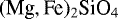 . Pyroxene can be Mg-pure MgSiO3 (enstatite), Fe-pure FeSiO3 (ferrosilite), or a combination of the two. The nomenclature En(x)Fs(1-x) indicates the fraction of iron (or magnesium) included in the compound. “En” stands for enstatite and “Fs” for ferrosilite. These silicate compounds are present in both crystalline and amorphous forms. We completed our sample set adding spinel, which is a Mg-bearing compound which crystallises in the cubic crystal system formed by oxygens, whereas Mg and Al atoms sit in tetrahedral and octahedral sites in the lattice (Mutschke et al. 1998). Spinel has been observed in chondritic meteorite with pre-solar composition and has been produced by gas outflows of red giant stars (Zinner et al. 2005).
2.2 Synchrotron measurements
Similar to the Si K-edge already presented by Zeegers et al. (2017, 2019), for the Mg K-edge we made use of the laboratory data that we obtained at the beamline LUCIA (Line for Ultimate Characterization by Imaging and Absorption; Flank et al. 2006) at the SOLEIL facility in Paris. The LUCIA X-ray microprobe is capable of performing spatially resolved chemical speciation via X-ray absorption spectroscopy (XAS). The 0.8− 8 keV X-raydomain of the tunable beam gives access to the K edges of low Z elements (from sodium up to iron) with a resolving power of about 4000. The measurements of the magnesium absorption edge are part of a larger synchrotron campaign inwhich the absorption edges due to Al and Si were also measured (Costantini et al. 2019; Zeegers et al. 2019).
The spectrum around the Mg K-edge was taken in the fluorescence geometry detecting the “secondary” (fluorescent) X-ray emission from the sample that has been excited by bombarding it with the synchrotron radiation. X-rays are energetic enough to expel tightly held electrons (photoelectron) from the inner orbitals (K-shell) making the electronic structure of the atom unstable. Consequently, one electron falls from a higher orbital level to the lower orbital to fill the hole left behind by a photoelectron. As a consequence, this releases fluorescent energy. This fluorescent signal can be used to derive the amount of absorption beyond the edge.
For each compound we took three to four measurements to average the signal and smooth out the possible small instrumental oscillations. Finally, we shifted our measurements by 2.54 eV to lower energies since the undulator radiation of the synchrotron introduced a systematic shift in the monochromator. In Appendix A we describe how we determined the exact value of thisenergy shift.
2.3 Extinction cross sections
To study the attenuation of X-rays by the interstellar dust, it is necessary to calculate the extinction cross section of each sample. We followed the same method already presented in Zeegers et al. (2017) and Rogantini et al. (2018). In this section, we summarise the procedure highlighting the most relevant steps. The main results are shown in the multiple panels of Fig. 1.
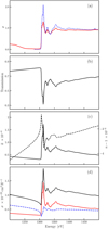 |
Fig. 1 Representation of data analysis for the forsterite Mg2SiO4. From top to bottom: (a) self-absorption correction: the synchrotron raw data (red solid line) and the signal corrected with the FLUO tool (blue dashed line).(b) Transmission for a thin layer (τ = 0.5 μm): the measured edge with XAFS (in black) are normalised using the tabulates values from Henke et al. (1993). (c) Optical constants: k is represented with the solid line while n − 1 with the dashed line (in units of 10−4). (d) The extinction (black solid), absorption (red solid), and scattering (blue dashed) cross sections per hydrogen nucleus for the Mathis, Rumpl, & Nordsieck (1977) dust model. |
Pile-up and self-absorption correction
Ideally, the samples should be either sufficiently thin or sufficiently diluted for the data to be unaffected by self-absorption effects. Practically, this may not be possible and the consequence would be an incorrect peak size in the XAFS. This is due to the variations in penetration depth into the sample as the energy is scanned through the edge and the finestructure (Tröger et al. 1992). Therefore, we corrected the spectrum using the standard FLUO algorithm3 , which is part of the UWXAFS analysis package (Stern et al. 1995). For comparison, we also used the tool ATHENA4 for the self-absorption correction, obtaining the same corrected signal (Ravel & Newville 2005). Finally, we also corrected the beamline data for any pile-up effect. For the Mg K-edge, this effect slightly distorts the region extending beyond the edge. In Fig. 1a we compare the raw data (solid red line) and the corrected data (dashed blue line). It is necessary toignore part of the pre-edge since the beamline was not yet stable during the measurement in this energy range.
Transmission
With the goal of determining the attenuation coefficient (μ) in μm −1 necessary tocalculate the refractive index of the material, we transformed the absorption in arbitrary units obtained from the fluorescent measurements into transmittance. We used tabulated values of the X-ray transmission of solids provided by the Centre for X-ray Optics at Lawrence Berkeley National laboratory5 (CXRO). In order to simulate the optically thin ISM condition, we chose a thickness of 0.5 μm; this value is far below the attenuation length of each sample. Knowing the transmittance (shown in Fig. 1b) it is possible to acquire the optical constants.
Optical constants
To obtain the extinction cross section of a specific material, it is fundamental to derive the refractive index. It is a complex and dimensionless quantity generally defined as m = n + ik. The imaginary absorptive part k is derived directly from the laboratory data, specifically from the transmittance signal. The real dispersive part n, on the other hand, can be calculated using the Kramers–Kronig relation (Kronig 1926; Kramers 1927). For this calculation we used the algorithm introduced by Watts (2014). The final results are shown in Fig. 1c. For further details on the calculation of the optical constants we refer to the dedicated paragraph in Rogantini et al. (2018).
Cross sections
To obtain the cross section from the optical constants, n and k, we employed the anomalous diffraction theory (ADT; van de Hulst 1957). This method allowed us to compute the absorption and scattering by dust grains of arbitrary geometry. In this step it is important to define the grain size range of interest. We calculated the scattering, absorption, and extinction cross sections (shown in Fig. 1d) for each compound via the standard Mathis–Rumpl–Nordsieck (MRN) grain size distribution (Mathis et al. 1977). See also Sect. 2.4.
Model in SPEX
Finally, we implemented the extinction profiles into the SPEX fitting code adding these to the library of amol (Pinto et al. 2010). Currently this model uses the Verner absorption curves (Verner et al. 1996). We adjusted the slopes of the pre- and post-edge of our extinction profiles avoiding any discontinuities between the XAFS data and the predefined curve in SPEX (Zeegers et al. 2017).
In Fig. 2 we compare, for illustrative purpose, the extinction cross sections of three representative compounds in our sample set: an amorphous Mg-pure pyroxene (blue dashed line), a crystalline Mg-pure olivine (red solid line), and the magnesium aluminium spinel (black solid line). The extinction cross sections of all the compounds are shown in Appendix B.
The chemical properties of the grains, in particular the length of the atom boundaries, determine the shape of the extinction profiles. Both olivine and pyroxene minerals, which share the same silicate tetrahedron, show similar patterns. Spinel, which instead presents an aluminium cubic structure, shows a distinct extinction shape and the main peak of the cross section is shifted at higher energy. The extinction cross section is also sensitive to the crystalline order of the mineral. Pure crystalline compounds shows multiple, distinct, and narrow peaks, whereas the extinction profiles of amorphous compounds are smoother and do not show any secondary peaks.
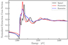 |
Fig. 2 Mg K-edge model implemented in SPEX for three different chemical compounds: crystalline spinel (MgAl 2 O4), crystalline forsterite (Mg2SiO4), and amorphous enstatite (MgSiO3). The major peak of spinel in the post-edge is shifted at higher energy with respect to the silicates. This is due to a different configuration of the atoms in the single unit cell. |
2.4 Large grain size distribution
In order to investigate the grain size, in particular focussing on the presence of particles larger than 0.25 μm, we calculateand implement in amol the extinction cross sections adopting a modified MRN grain size distribution. Specifically, we adopt the distribution already presented by Zeegers et al. (2017) with (0.05 ≤ a ≤ 0.5) μm. In Fig. 3 we show the effect of this change in the grain size distribution. The forsterite Mg K-edge with a MRN distribution with particle size of 0.005−0.25 μm is shown in black and in red the same edge but now with a LMRN size distribution that has a particle size in the range 0.05−0.5 μm. The feature before the edge (~1305 eV), namely the scattering peak, is sensitive to the dust grain size and it is due to an enhanced scattering efficiency for larger grain size (Zeegers et al. 2017; Rogantini et al. 2018).
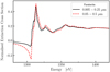 |
Fig. 3 Normalised extinction cross section for forsterite using two different grain size distributions. The solid black line represents the standard MRN grain size in the range 0.005− 0.25 μm. The dashed red line delineates the larger grain size spanning 0.05−0.5 μm. |
2.5 Magnesium and silicon models
In this paper, for the first time, we simultaneously analyse the magnesium and silicon K-edges of a bright LMXB. We built our extinction model joining the laboratory cross sections of the Mg K-edge, from the present work, together with the Si K-edge cross sections taken from Zeegers et al. (2017, 2019). The extinction models with both Mg and Si K-edges were implemented in the amol model. Moreover, we included in our models the Si-bearing compounds that do not contain magnesium in molecules such as quartz and fayalite. We also added magnesium oxide (also known as magnesia), which contains only magnesium (Fukushi et al. 2017). Since the Si K-edge model of hypersthene is not available (Zeegers et al. 2019), we did not use this compound during the analysis and we just present its Mg K-edge cross-section. Moreover, we did not include spinel in the fitting of the astronomical data. This is because the aluminium in the compound could be misquantified as a consequence of possible calibration residuals in the Al edge6 of the source spectrum. We report, in Table 1 (with the index #Mod), the complete list of the extinction profiles used to analyse the Mg and Si K-edges ISM absorption observations.
3 Astronomical observation
3.1 GX 3+1
We used the bright X-ray binary GX 3+1 as a test source. This source has a persistent bolometric luminosity of ~ 6 × 1037 erg s−1 (den Hartog et al. 2003) and the spectrum shows deep Mg and Si absorption edges at 1.308 and 1.840 keV (9.50 and 6.74 Å), respectively. GX 3+1 (also known as Sgr X-1 and 4U 1744-26) is one of the first discovered cosmic X-ray sources. This X-ray binary was detected during an Aerobee-rocket flight on June 16, 1964 (Bowyer et al. 1965). Ever since this initial observation, this source has been intensely observed with multiple satellites: i.e. Hakucho (Makishima et al. 1983), Granat (Lutovinov et al. 2003), Ginga (Asai et al. 1993), Rossi X-ray Timing Explorer (RXTE, Kuulkers & van der Klis 2000), Beppo-SAX (Oosterbroek et al. 2001; den Hartog et al. 2003; Seifina & Titarchuk 2012), Integral (Chenevez et al. 2006), XMM-Newton (Piraino et al. 2012; Pintore et al. 2015), and Chandra (Schulz et al. 2016). The detection of multiple thermonuclear bursts (Makishima et al. 1983; Kuulkers 2002) suggests that the compact object hosted in GX 3+1 was an accreting neutron star. Thanks to the detection of these X-ray bursts with radius expansion the distance to the source was estimated to be in the range 4.2−6.4 kpc with a best estimate of ~6.1 kpc (Kuulkers &van der Klis 2000; den Hartog et al. 2003). Spectral analysis of the source showed that its X-ray spectrum can be described by a model comprised of a black-body component, which is most likely associated with the accretion disc; and a Comptonised component, which is produced by an optically thick electron population located close to the neutron star corona (Oosterbroek et al. 2001; Mainardi et al. 2010; Seifina & Titarchuk 2012).
3.2 Datareduction
We used seven datasets from Chandra (see Table 2), taken in timed exposure (TE) mode between July 2014 and May 2017, for a total exposure of ~213 ks. The spectrum has been observed by the High Energy Transmission Grating (HETG) instrument of Chandra (Canizares et al. 2005). Each dataset contains both High Energy Grating (HEG) and Medium Energy Grating (MEG) grating spectra which have been downloaded from the Chandra Grating-Data Archive and Catalogue (TGCat; Huenemoerder et al. 2011). Using the Chandra Interactive Analysis of Observations (CIAO; Fruscione et al. 2006) we combined the +/− first order for each HEG and MEG observation. The HEG and MEG spectra of a single observation are fitted together with the same model, correcting their instrumental normalisations when necessary. In total, we fit 14 spectra simultaneously.
The average count rate is ~100 counts per second, which translates to a flux of ~4.7 × 10⁻⁹ erg s−1 cm−2 in the range 2−10 keV (Oosterbroek et al. 2001). The observations are affected by pile-up because of this high flux. The bulk of the pile-up photons come from the MEG first order where the Si K edge resides on a back-illuminated CCD. The High Energy Transmission Grating Spectrometer (HETGS) has a high effective area between 1 and 3 keV, and we excluded some of the data (E > 1.55 keV). For HEG we consider the broad energy band in the range 1.1−5.2 keV (~ 2.4−10.8 Å, respectively).
Samples in our set with their relative chemical formula, form, origin, and reference index.
Broadband modelling of GX 3+1 using HEG and MEG data of seven observations.
3.3 Continuum
We assumed the presence of both thermal and non-thermal emission to represent the continuum of GX 3+1 (Mitsuda et al. 1984). Among the thermal components present in SPEX we tested a black body (bb; Kirchhoff & Bunsen 1860), a disc-black body (dbb; Shakura & Sunyaev 1973; Shakura 1973), and a black body modified by Compton emission (mbb; Rybicki et al. 1986; Kaastra & Barr 1989). We tested non-thermal components of the power law (pow) and the Comptonisation model (comt, Titarchuk 1994). The best-fit model for GX 3+1 shows a black body plus a power law absorbed by a cold absorbing neutral gas model, simulated by the hot model in SPEX (de Plaa et al. 2004; Steenbrugge et al. 2005).
For the cold absorption model, we fixed the electron temperature at the lower limit of the hot model, that is Te = 0.5 eV. We updated the photo-absorption cross section of neutral magnesium in SPEX, adding the resonance transitions, 1s → np, calculated using the Flexible Atomic Code7 (A. Raassen, priv. comm.). Our neutral Mg K-shell cross section is consistent with the Mg I profile obtained by Hasoğlu et al. (2014) applying the R-matrix method.
We simultaneously fitted the multiple datasets by coupling the absorption by neutral gas in the interstellar matter that we assume to be constant. The model was fitted to the data using the C-statistic (Cash 1979). Using the abundances tabulated by Lodders (2010), we obtained a hydrogen column density NH = (1.91 ± 0.05) × 1022 cm−2 that is consistent with the values of previous works. The average best fit of the continuum is represented in Fig. 4 and the parameter values for each observation are reported in Table 2. The residuals in the Mg and Si K-edge region hint that weare overestimating the content of these two elements in the gas phase. Thus, it is necessary to add the dust model to fit the residuals present.
Furthermore, we tested the presence of collisionally ionised gas along the line of sight and the gas outflow from the source in its environments. Thus, we added an extra hot component plus the photo-ionised absorption model (xabs in SPEX, Steenbrugge et al. 2003) to our model. We did not find any evidence of ionised gas along the line of sight.
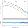 |
Fig. 4 Continuum of GX 3+1. HEG (light blue) and MEG (dark blue) data from seven datasets were used to fit the continuum. We stacked and binned the observations for display purpose only. The average fit of the seven data sets is shown with a red solid line. The model consists of a black body (in black) and a power law (green) with a photoelectric absorption component with NH ≃ 1.9 × 1022 cm−2. In the bottom panel we show the relative residuals defined as (observed-model)/error. The residual around 8 Å is due to the uncertainty on calibration for the aluminium K-edge. |
3.4 Fit of the magnesium and silicon edges
After studying the continuum we fitted our dust models to Chandra-HETG data to study the solid phase of the ISM along the line of sight.In the fit we kept the temperature and the power-law index of the continuum model, leaving the respective normalisations free to vary.
The dust models necessary to characterise the near-edge features of the Si and Mg K-edges were implemented in the multiplicative component amol. This SPEX model can fit a dust mixture consisting of four different types of dust at the same time. We followed the same method as described in Costantini et al. (2012), in which they tested all the possible configurations of the dust species and compared all the outcomes using a criterion based on the C-statistics value (see Sect. 3.5). The number of compound combinations is given by
 (1)
(1)
where n is the number of compounds and k the combination class. Since each combination describes a single extinction model, Cn,k represent the number of models utilised to fit the data.
Initially, only the extinction models obtained assuming the MRN size distribution (n = 15) were selected to study the XANES profiles at the Mg and Si K-edges. In Fig. 5 we show the best fit of the two X-ray edges with the green solid line. The C-statistic (Cstat) value is 28 199 with 27 207 degrees of freedom (d.o.f). The mixture that fits the data best consists mainly of amorphous olivine (~ 85%) and a smaller contribution of magnesium oxide.
Furthermore, we tested a different size distribution fitting the data using exclusively extinction cross sections obtained adopting the LMRN size distribution (n = 15), presented in Sect. 2.3. The relative best fit, with a Cstat/d.o.f equivalent to 28 182/27 207, is shown in Fig. 5 with the blue solid line. The C-stat improves with LMRN. However this fit requires a large amount of gas, for both Mg and Si, in order to fit the data (30 and 40%, respectively). This is difficult to reconcile with literature values (Jenkins 2009).
In the final analysis we considered both dust size distributions for all our measurements (n = 30). The best fit, with a Cstat value of 28 129/27 207, is represented with the red solid line. The relative residuals (for both HEG and MEG) are shown in the bottom panel. The dust that best represents the data is a mixture of amorphous olivine (~ 71%), crystalline fayalite (~ 16%), and amorphous quartz (~ 13%). The contribution of MRN and LMRN size distribution models is comparable at ~57 and ~43%, respectively.The Si K-edge shows further residuals around the energy threshold. We discuss these residuals further in Sect. 4.1.
The mixture of standard and large MRN grains gives the best representation of the Mg and Si K-edges. The parameter values for the LMRN + MRN, MRN, and LMRN models with their statistical errors are summarised in Table 3. For clarity we divided the table into blocks. In the upper block of the table N1−4 indicate thecolumn density of each dust species present in the model in units of 1017 cm−2. In the second block we list the gaseous phase column density of each element of interest (NX).
We summarise, in Table 4, the depletion values and total abundances for oxygen, magnesium, silicon, and iron. The abundances are calculated considering the total amount of atoms in both the gas and solid phases and these are compared with the solar abundances from Lodders (2010).
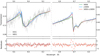 |
Fig. 5 Top panel: magnesium and silicon K-edges of GX 3+1. The HEG and MEG data are shown in light and dark grey, respectively. We do not consider MEG data for the Si K-edge because of the pile-up contamination. We fit the two edges using models with different grain size distributions: MRN models only in green, LMRN models only in blue, and both MRN and LMRN models in red. Bottom panel: we show the residuals defined as (observed-model)/error of the best fit obtained using MRN and LMRN models. The HEG and MEG data are shown in light and dark red, respectively. The data are stacked and binned for display purposes. |
Dust and gas column densities obtained by fitting the Mg and Si K-edges.
Abundances and fractional depletions.
3.5 Evaluating the goodness of fit
Consideringall the models calculated using both MRN and LMRN size distributions, we obtained 27 405 models (from Eq. (1)). The C-statistics values representative of different dust mixtures can be similar. Since our candidate models are not-nested and with same number of free parameters, the standard model comparison tests (e.g. the χ2 goodness-of-fit test, the maximum likelihood ratio test, and the F-test) cannot be used to evaluate the significance of the models (Protassov et al. 2002). The Aikake Information Criterion (AIC)8 represents an elegant estimator of the relative quality of not-nested models without relying on time-consuming Monte Carlo simulations (Akaike 1974, 1998). The AIC value of a model is defined as
 (2)
(2)
where k is the number of fitted parameters of the model and  maximum likelihood value. Recalling the relation
  (Cash 1979) the relation between C-statistic and AIC is clear.
In our work it is not the absolute size of the AIC value, but rather the difference between AIC values (ΔAIC), that is important. The AIC difference, defined as
![Mathematical equation: \[ \Delta {\textrm{AIC}}_{i} = \textrm{AIC}_{i} - \textrm{AIC}_{\textrm{min}}, \]](/articles/aa/full_html/2019/10/aa35883-19/aa35883-19-eq8.png)
allows for a comparison and ranking of the candidates models. For the model estimated to be best, ΔAICi ≡ ΔAICmin ≡ 0. Following the criteria presented in Burnham & Anderson (2002), we considered competitive with the selected best model the models with ΔAICi < 10.
From the AIC-selected models, we obtained the relative contribution of each dust compound over the total dust obscuration.In Fig. 6 we show the relative fraction of the dust species for both MRN (lighter colour) and LMRN (darker colour) dust size distributions. The red-highlighted bar indicates the compounds for which we are able to constrain their relative contribution. The amorphous olivine is the most representative compound among the selected models and has a relative value of 0.70 ± 0.09 (0.43 ± 0.04 and 0.27 ± 0.08 for the MRN and LMRN size distributions, respectively). In particular, the amorphous olivine (a-olivine) is the major contributor for every AIC-selected model. Models without any important contribution from a-olivine show ΔAICi > 35.
A secondary contribution is given by the crystalline fayalite, which has a LMRN size distribution, which represents a relative value of 0.091 ± 0.088. For the remaining compounds we obtained the upper limits (grey bars in Fig. 6) of their contributions, which are always lower than 0.07. Regarding the compounds listed in Table 1 and missing in Fig. 6 (i.e. a-enstatite, c-En60Fs40, c-En90Fs10, a-forsterite, and c-olivine), they do not occur in any of the selected models and we consider their contributions negligible in this fit.The models selected with the AIC method agree not surprisingly with the best fit obtained with the Cstat.
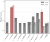 |
Fig. 6 Bar plot of the relative abundance for each dust species calculated considering AIC-selected models. Darker bars represent models with a LMRN size distribution; lighter bars refer to MRN models. We highlight the dust species with a constrained relative fraction with red filled bars. |
4 Discussion
4.1 Silicon edge residuals
The HETG/Chandra data in GX 3+1 exhibit a peculiar shape of the pre-edge region of silicon K transition. In Fig. 7 we show a zoom-in of the silicon K-edge. The complexity of this edge was already observed by Schulz et al. (2016). With our larger set of observations (approximately a double exposure time) we observed this complex structure with a significance ≳ 5σ. Schulz et al. (2016) inferred that the peak centred at 6.740 Å is due to X-ray scattering. However, its wavelength does not correspond to the scattering peak of our dust extinction model, which is instead centred at 6.728 Å. It is possible that the peak is contaminated by an unresolved and unknown instrumental artefact (Miller et al. 2002). Regarding the absorption present right before the onset of the edge, we speculate that its origin is attribute to ISM present along the line of sight and we tested different possibilities.
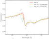 |
Fig. 7 Zoom-in of the silicon K-edge. We represent the best fit with a red solid line. We show, in orange, the model obtained byadding secondary Si-bearing dust candidates presented in the text to the best fit. The green dashed line represents the best fit adding the neutral silicon cross section calculated with the COWAN code. We use a data bin size of ~ 0.04 Å, approximately one-third full width half maximum (in other words the energy resolution of the detector). |
Neutral silicon
The K-shell X-ray absorption for a single, isolated silicon atom presents multiple resonance transitions 1s → 3p. We updated the Verner et al. (1996) silicon cross section present in SPEX with these transitions, calculated using both the FAC and COWAN codes (Cowan 1981, A. Raassen, priv. comm.). Assuming the silicon depletion value found in the best fit (δSi = 0.94), with the update cross section we obtained an absorption feature with a strength similar to the absorption feature observed right before the onset of the Si K-edge. However, none of these absorption features correspond exactly to the energy measured by HETG: the absorption line calculated with the two different codes are shifted to lower energies (higher wavelengths) of ΔE ~ 1.5−4.5 eV (Δλ ~ 0.006−0.017 Å). These shifts are noticeable since the differences are close to the energy resolution of HEG in the silicon region (Δλ = 0.012 Å). In Fig. 7 the green dashed line shows the absorption line due to the resonance transitions calculated with the COWAN code, which presents the less divergent shift. Moreover, Hasoglu & Gorczyca (2018) calculated the K-shell photo-absorption of neutral silicon using a modified version of the R-Matrix method (Berrington et al. 1995). Their final result is somewhat consistent to our calculation using the COWAN code.
Ionised gas
We tested if a photo-ionised gas is able to reproduce the absorption feature right before the onset of the edge. Thus, we added a photo-ionised component (xabs in SPEX) with a systematic velocity that is free to vary to our model. This results in a modest column density ( ) for an ionisation parameter of
  .
.
We also tested collisional ionised plasma (component hot in SPEX), with a temperature constrained between 0.3 and 2 keV, to ensure absorption by SiXIII in the Si K-edge region, obtaining an upper limit for the column density (NH < 1.5 × 1020 cm−2).
Si-bearing dust
In the interstellar dust, silicon is potentially able to create a chemical bound with different elements than oxygen, the standard characteristic bond of silica and silicates. Therefore, we included in our Si K-edge model set cosmic dust candidates such as crystalline silicon (Witt et al. 1998; Li & Draine 2002), crystalline silicon carbide (SiC; Whittet et al. 1990; Min et al. 2007), and silicon nitride (Si3 N4; Jones 2007)9. The Si–Si, Si–C, and Si–N bonds are characterised by lower energy thresholds and consequently, their Si K-edges are wavelength-shifted with respectto those of the silicate. We added magnesia (MgO) to our model to compensate for any silicate-poor (and therefore magnesium poor) fittingthat we tested. The resulting model is presented in Fig. 7 with a orange solid line. The fit has a better C-statistic value but a lower AIC value owing to the penalty term 2k in Eq. (2).
Double silicate edge
We naively added a supplementary silicate component with systematic velocity free to vary to our best model and this resulted in a relative large amount of cold material (NH ~ 3 × 1017 cm−2) with a receding velocity ≳500 km s−1 along the line of sight. This scenario is hard to justify since such motion of matter is not observed the literature (e.g. van den Berg et al. 2014; Pintore et al. 2015) and furthermore the magnesium K-edge does not show an evident additional, redshifted feature.
We can also discarded porosity and different grain geometries as possible cause of the residuals since Hoffman & Draine (2016) showed that their effects on the silicon edge profile is negligible. Presently, we are not able to characterise the features located next to the onset of the Si K-edge between 6.72 and 6.75 Å. The comparison of the Mg and Si K-edges detected in different lines of sight will be crucial to understand the nature of it in forthcoming works.
4.2 Depletions and abundances
By fitting the low energy curvature of the X-ray spectrum of GX 3+1 and adopting the proto-solar abundances of Lodders (2010), we find a hydrogen column density of NH = (1.91 ± 0.02) × 1022 cm−2. Using the solar abundances of Anders & Grevesse (1989), adopted by previous authors, this value corresponds to ~ 1.61 × 1022 cm-2 and is consistent with the neutral column density obtained by Oosterbroek et al. (2001), where NH = (1.59 ± 0.12) × 1022 cm−2. From the residuals of the continuum analysis in Fig. 4, it is clear that the silicon and magnesium edges cannot be represented only by pure gas absorption and it is necessary to introduce the dust component by adding amol to the fitting model. The dust models used in the analysis (see Table 1) contain oxygen, magnesium, silicon, and iron. The content of these elements in the solid phase is expressed by the depletion values shown in Table 4.
Silicon is highly depleted along the line of sight of the source: more than 90% is found in the solid phase. Similarly, a high percentage of magnesium (more than 80%) is included in dust grains. The two elements share the similar depletion values, which is in agreement with the fractional depletion observed by Dwek (2016) and Jenkins (2009). The depletions of oxygen and iron in dust are derived indirectly from the model since the absorption edges of these elements fall outside the spectral band. Therefore, no strong conclusions can be drawn regarding these two elements. However, oxygen shows a moderate fractional depletion value (δO = 0.27 ± 0.02). This value would be consistent with the depletion observed for lines of sight with different neutral column densities (e.g. Costantini et al. 2012; Pinto et al. 2013), confirming the weak correlation between the depletion of oxygen and the physical conditions of the environment (e.g. density and temperature; Whittet 2002). Instead, iron seems highly depleted consistently with the values shown by Whittet (2002) and Jenkins (2009).
The total abundances were evaluated by summing the column densities of the gas and solid phases for each element. Our values do not depart significantly from the solar values (see Table 4).
4.3 Dust chemistry
The simultaneous analysis of the silicon and magnesium edges is in principle able to constrain the typical cations-to-silica ratio (Mg+Fe)/Si of interstellar silicate grains. For the best fit of the data we find that (Mg + Fe)/Si ~ 2, considering only pyroxene and olivine compounds. This gives O/Si = 4, implying that silicates along the line of sight present an olivine-type stoichiometry. Indeed, the amorphous and crystalline olivine, together with the fayalite, are characterised by the orthosilicate anion [SiO ] and represent ~91% of the dust in our fit.
Moreover, the best fit is characterised by Mg∕(Mg + Fe) = 0.41 ± 0.02 (and therefore by Mg : Fe = 0.69 ± 0.05). Fayalite gives the major contribution of iron for the dust component and it is preferred over the magnesium-rich forsterite. We found a larger presence of iron in silicates with respect to the values observed for different lines of sight (e.g. Costantini et al. 2012), wavelengths (e.g. Tielens et al. 1998; Min et al. 2007; Blommaert et al. 2014), and/or environments (e.g. the interplanetary medium; Altobelli et al. 2016), where Mg-rich silicates are detected. However, we cannot constrain the iron depletion value since we cannot characterise the iron absorption edges directly and simultaneously. The analysis of the AIC-selected models shows similar ratios (namely, (Mg + Fe)/Si ≈ 1.9; Mg ∕(Mg + Fe) ≈ 0.45; Mg ∕Fe ~ 0.8), which agrees with the nominal best-fitting model.
4.4 Dust crystallinity
The best fit suggests the presence of a relatively large amount of crystalline grains along the line of sight of GX 3+1. Defining the crystalline-to-amorphous ratio as ζ1 = crystalline dust/(crystalline dust + amorphous dust) (Zeegers et al. 2019), we find a value of ζ1 = 0.15 ± 0.03. This is consistent to the range of values found by Zeegers et al. (2019), ζ1 = 0.04−0.12, using several several LMXBs. Comparing our results with the literature, we find higher percentages of crystalline dust with respect to the fractions observed by the infrared spectroscopy. For example, Li et al. (2007), Kemper et al. (2004), analysing the 9.7 μm and 18 μm features, set the possible maximum crystalline fraction of the total silicate mass in the ISM to a maximum of 5% and 1.1%, respectively.
The crystalline ratio that we find may be partially biased by the limitation of our measured set of compounds. Previous works already showed and discussed the presence of this bias (Zeegers et al. 2017). Indeed, our laboratory model set does not include the amorphous counterpart for all the compounds (see Table 1) and consequently, the estimation of the crystallinity may be overestimated. Indeed, in our case, the crystalline ratio is led by the crystalline fayalite, for which the amorphous counterpart, which might contribute to the total fit, is not available.
However, if this observed amount of crystalline dust is real, the differences with the infrared observations might be explained in two possible ways. The first is that cold and dense regions, accessible only by X-rays, host cosmic dust with a different crystalline order with respect to the grains which populate the diffuse medium. These differences could be explained by the theoretical model presented by Tanaka et al. (2010) and Yamamoto et al. (2010), which predict a low-temperature crystallisation of amorphous silicate grains induced by exothermic chemical reactions. An alternative explanation is that we might be detecting poly-mineralic silicates, which are expected to be agglomerated particles, possibly containing both crystalline and glassy constituents. In this case, because X-rays are sensitive to a short-range order, XAFS would show crystalline features, whereas there might not be sharp crystalline features in the infrared spectrum Speck et al. (2011).
4.5 Dust size
The best fit of the magnesium and silicon K edges is obtained assuming the existence of two dust populations with different size distributions: MRN and LMRN presented inSect. 2.3. From the results of analysing the two X-ray edges, the two distributions show similar weights with MRN∕(LMRN + MRN) ~ 0.57.
This approach was motivated by the known complexity of the line of sight towards GX 3+1, which is at a distance of about 6.1 kpc (Kuulkers & van der Klis 2000) and at longitude l = 2.29 and latitude b = 0.79 in galactic coordinates (Ebisawa et al. 2003). Therefore, assuming a distance towards the Galactic centre of 8.5 kpc, the source is located in the outskirts of the Galactic bulge. In particular, this source is situated just behind the “near 3 kiloparsec arm”, which is expanding at a speed of ~57 km s−1 (van Woerden et al. 1957; Dame & Thaddeus 2008), and the molecular ring (Clemens et al. 1988; Jackson et al. 2006), located at a distance of 5.5 and 5 kpc from the Sun, respectively. The CO emission in these latter two regions is clumped (Bania 1980). In particular, the molecular ring contains about 70% of all the molecular gas inside the solar circle (Clemens et al. 1988). The ring is thus an enormous reservoir of material in gaseous and solid form. Moreover, GX 3+1 is aligned with the known Bania’s Clump 2, a molecular cloud complex near the Galactic centre (Bania 1977; Stark & Bania 1986). Several dust lanes in the Galactic bar seem to be connected with this feature (Liszt 2008). However, because of the uncertainties on the distance estimate, it is unclear if our source is embedded in these structures or if it is in front of them (Marshall et al. 2008).
Within 5 kpc from the Sun the line of sight crosses several spiral arms (located at different solar distances; Benjamin 2008; Urquhart et al. 2014): i.e., Sagittarius–Carina (~ 1.5 kpc), Scutum–Centaurus (~ 3.5 kpc), and Norma arms (~4.5 kpc).
In this scenario, diffuse dust with a MRN distribution would be naturally located within the spiral arms. The large dust population, containing mainly amorphous olivine and fayalite, would instead probably belong to the molecular regions close to the Galactic centre. Here, shielded from dissociating interstellar radiation, the dust grains can easily grow (e.g. Chapman et al. 2009; Hirashita 2012). The presence of large grains in these regions is thought to be supported by the “core shine” effect seen in mid- and near-infrared observations of dark clouds (e.g. Pagani et al. 2010; Lefèvre et al. 2014).
Moreover, at these particular coordinates, the 3D polarisation model, developed by Martínez-Solaeche et al. (2018) taking into account observed dust emission and observed intensity and polarisation power spectra, shows an enhanced polarisation vector P at distance ≳ 3.8 kpc. As found by Kim & Martin (1995) the astronomical silicates of a > 0.1 μm n size can reproduce the observed polarisation of the starlight.
Finally, previous works have already observed the presence of different dust populations distributed along the line of sight. Recently, Vasilopoulos & Petropoulou (2016) analysed the X-ray dust-scattered rings from the LMXB V404 Cyg. These authors found that the dust grains are concentrated in different dust layers each characterised by a different size distribution. However, future works, using different grain size distributions such as Weingartner & Draine (2001), Zubko et al. (2004), and The Heterogeneous dust Evolution Model for Interstellar Solid (THEMIS, Jones et al. 2013; Köhler et al. 2014) as well as an in-depth understanding of the instrument around crucial edges, will be necessary to study the dust distribution in detail.
5 Conclusions
In this paper we present the first attempt to build an X-ray broadband extinction model with multiple edges. In particular, in this work we focus on the simultaneous modelling of the magnesium and silicon extinction profiles both based on synchrotron measurements. This approach allows us to better constrain the cosmic dust properties and to avoid degeneracies that can occur using a single edge fit.
We introduce the Mg K-edge extinction cross sections of 12 different dust species focussing on their XANES profiles. We analyse the X-ray spectrum of the bright LMXB GX 3+1, whose hydrogen column density is optimized for the simultaneous detection of the magnesium and silicon edges, and we characterise the gas and dust along the line of sight. Below we summarise the main results.
-
The absorption spectrum shows the presence of both gas and dust along the line of sight. We find standard solar abundances of magnesium and silicon (AMg∕A⊙ = 0.88 ± 0.08 and ASi∕A⊙ = 1.21 ± 0.10) and their relative depletion values are in agreement with the results obtained by Jenkins (2009) (δMg = 0.89 ± 0.10 and δSi = 0.94 ± 0.6).
-
We find that amorphous olivine is the most representative dust species along the line of sight of GX 3+1. The olivine orthosilicates characterised by the anion SiO4 are highly preferred over silica (SiO2) and pyroxene (SiO3). For the best fit we find a cations-to-anion ratio of (Mg + Fe)/Si ~ 2.
To fully characterise the silicon and magnesium K-edges and in view of future X-ray missions with better resolving power (XRISM and Athena) it is necessary to develop accurate and detailed cross sections of neutral gas. Those can indeed explain the residuals that we still find in our analysis in the Si K-edge region and they will help to determine the depletion values of the respective elements. Moreover it is also crucial to understand if the pre-edge of the silicon K-edge is contaminated by possible instrumental artefacts and how these affect the modelling of dust extinction.
Acknowledgements
D.R., E.C., I.P., and M.M. are supported by The Netherlands Organisation for Scientific Research (NWO) through The Innovational Research Incentives Scheme Vidi grant 639.042.525. The Space Research Organization of the Netherlands is supported financially by NWO. We acknowledge SOLEIL for provision of synchrotron radiation facilities and we thank Delphine Vantelon for assistance in using the beamline LUCIA. This research has made use of data obtained from the Chandra Data Archive and the Chandra Source Catalog, and software provided by the Chandra X-ray Center (CXC) in the application package CIAO. We are grateful to the referee for valuable comments that lead to improvements of the paper. We thank A.J.J. Raassen for providing the photo-absorption cross section of neutral magnesium and silicon. We are grateful to P. Ranalli for useful discussions. We also thank A. Dekker and D. Lena for reading an early draft of the manuscript and for providing valuable comments and suggestions.
Appendix A Mg K-edge shift
Comparing our synchrotron measurements with previous and independent works we notice a discrepancy in the energy of the magnesium K-edge threshold. In particular, in Fig. A.1 we compare the normalised XANES spectra of crystalline forsterite. We show the result of our measurements with the XANES profiles obtained by Wu et al. (2004), Trcera et al. (2009), and Takahashi et al. (2018). Our result appears shifted to higher energies with respects to the other reference XANES spectra. We chose to evaluate the energy shift calibrating our model on the spectrum of GX 3+1 presented in this paper in Sect. 2. We set the systematic velocity of the absorber (zv parameter in AMOL) as a free parameter and we run the fit of the magnesium K-edge using a combination of all the minerals (see Eq. (1)). This approach to define the absolute energy value of a particular transition (difficult to define by experimental data and/or calculations) was already adopted by Gorczyca et al. (2013) for the atomic oxygen. We selected the models with a ΔAIC < 2 (Burnham & Anderson 2002) from the best fit and we found an average speed of zv = −585 km s−1 corresponding to an energy shift of E = −2.54 eV in the Mg K-edge region. This value is in agreement with previous works shown in Fig. A.1.
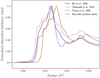 |
Fig. A.1 XANES spectra of crystalline forsterite at the Mg K-edge. Experimental spectra from different works are listed in the panel. |
Appendix B Extinction cross sections of the Mg Kedges
In Fig. B.1 we present the extinction cross section profiles around the magnesium K-edge for each sample presented in Table 1. The measurements were taken at SOLEIL (Paris). We adopt the standard MRN size distribution (Mathis et al. 1977) to obtain the extinction cross sections. These curves were implemented in the amol model of the spectral fitting code SPEX with a fixed energy resolution of 0.1 eV. The absorption, scattering, and extinction cross sections of the compounds (with an energy range between 1100 and 1550 eV) are available in ASCII format10 .
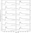 |
Fig. B.1 Mg K-edge extinction cross sections of the mineral compounds presented in this work and listed in Table 1. |
References
- Akaike, H. 1974, IEEE Trans. Automat. Contr., 19, 716 [Google Scholar]
- Akaike, H. 1998, Prediction and Entropy, eds. E. Parzen, K. Tanabe, & G. Kitagawa (New York: Springer New York), 387 [Google Scholar]
- Altobelli, N., Postberg, F., Fiege, K., et al. 2016, Science, 352, 312 [NASA ADS] [CrossRef] [Google Scholar]
- Anders, E., & Grevesse, N. 1989, Geochim. Cosmochim. Acta, 53, 197 [Google Scholar]
- Asai, K., Dotani, T., Nagase, F., et al. 1993, PASJ, 45, 801 [NASA ADS] [Google Scholar]
- Bania, T. M. 1977, ApJ, 216, 381 [NASA ADS] [CrossRef] [Google Scholar]
- Bania, T. M. 1980, ApJ, 242, 95 [NASA ADS] [CrossRef] [Google Scholar]
- Benjamin, R. A. 2008, ASP Conf. Ser., 387, 375 [NASA ADS] [Google Scholar]
- Berrington, K.A., Eissner, W. B., & Norrington, P. H. 1995, Comput. Phys. Commun., 92, 290 [NASA ADS] [CrossRef] [Google Scholar]
- Bilalbegović, G., Maksimović, A., & Valencic, L. A. 2018, MNRAS, 476, 5358 [NASA ADS] [CrossRef] [Google Scholar]
- Blommaert, J.A. D. L., de Vries, B. L., Waters, L. B. F. M., et al. 2014, A&A, 565, A109 [NASA ADS] [CrossRef] [EDP Sciences] [Google Scholar]
- Bowyer, S., Byram, E. T., Chubb, T. A., & Friedman, H. 1965, Science, 147, 394 [NASA ADS] [CrossRef] [Google Scholar]
- Bunker, G. 2010, Introduction to XAFS (Cambridge, UK: Cambridge University Press) [CrossRef] [Google Scholar]
- Burnham, K. P., & Anderson, D. R. 2002, Model Selection and Multimodel Inference: a Practical Information-theoretic Approach, 2nd edn. (Berlin: Springer), 1 [Google Scholar]
- Canizares, C. R., Davis, J. E., Dewey, D., et al. 2005, PASP, 117, 1144 [NASA ADS] [CrossRef] [Google Scholar]
- Cash, W. 1979, ApJ, 228, 939 [NASA ADS] [CrossRef] [Google Scholar]
- Chang, Y., Hsieh, H.-H., Pong, W.-F., et al. 1999, J. Appl. Phys., 86, 5609 [NASA ADS] [CrossRef] [Google Scholar]
- Chapman, N. L., Mundy, L. G., Lai, S.-P., & Evans, II, N. J., 2009, ApJ, 690, 496 [NASA ADS] [CrossRef] [Google Scholar]
- Chenevez, J., Falanga, M., Brandt, S., et al. 2006, A&A, 449, L5 [NASA ADS] [CrossRef] [EDP Sciences] [Google Scholar]
- Clemens, D. P., Sanders, D. B., & Scoville, N. Z. 1988, ApJ, 327, 139 [NASA ADS] [CrossRef] [Google Scholar]
- Corrales, L. R., & Paerels, F. 2015, MNRAS, 453, 1121 [NASA ADS] [CrossRef] [Google Scholar]
- Costantini, E., & de Vries, C. P. 2013, Mem. Soc. Astron. It., 84, 592 [Google Scholar]
- Costantini, E., Pinto, C., Kaastra, J. S., et al. 2012, A&A, 539, A32 [NASA ADS] [CrossRef] [EDP Sciences] [Google Scholar]
- Costantini, E., Zeegers, S. T., Rogantini, D., et al. 2019, A&A, 629, A78 [NASA ADS] [CrossRef] [EDP Sciences] [Google Scholar]
- Cowan, J. 1995, The Biological Chemistry of Magnesium (Hoboken, NJ: Wiley) [Google Scholar]
- Cowan, R. D. 1981, The Theory of Atomic Structure and Spectra (Berkeley, CA: University of California Press) [Google Scholar]
- Dame, T. M., & Thaddeus, P. 2008, ApJ, 683, L143 [NASA ADS] [CrossRef] [Google Scholar]
- den Hartog, P. R., in’t Zand, J. J. M., Kuulkers, E., et al. 2003, A&A, 400, 633 [NASA ADS] [CrossRef] [EDP Sciences] [Google Scholar]
- de Plaa, J., Kaastra, J. S., Tamura, T., et al. 2004, A&A, 423, 49 [NASA ADS] [CrossRef] [EDP Sciences] [Google Scholar]
- Draine, B. T. 2003, ApJ, 598, 1026 [NASA ADS] [CrossRef] [Google Scholar]
- Dwek, E. 2016, ApJ, 825, 136 [NASA ADS] [CrossRef] [Google Scholar]
- Ebisawa, K., Bourban, G., Bodaghee, A., Mowlavi, N., & Courvoisier, T. J.-L. 2003, A&A, 411, L59 [NASA ADS] [CrossRef] [EDP Sciences] [Google Scholar]
- Fabian, D., Jäger, C., Henning, T., Dorschne, J., & Mutschke, H. 2000, ESA SP, 456, 347 [NASA ADS] [Google Scholar]
- Flank, A.-M., Cauchon, G., Lagarde, P., et al. 2006, Nucl. Instrum. Methods Phys. Res. B, 246, 269 [NASA ADS] [CrossRef] [Google Scholar]
- Fruscione, A., McDowell, J. C., Allen, G. E., et al. 2006, Proc. SPIE Conf. Ser., 6270, 62701V [Google Scholar]
- Fukushi, K., Suzuki, Y., Kawano, J., et al. 2017, Geochim. Cosmochim. Acta, 213, 457 [NASA ADS] [CrossRef] [Google Scholar]
- Gorczyca, T. W., Bautista, M. A., Hasoglu, M. F., et al. 2013, ApJ, 779, 78 [NASA ADS] [CrossRef] [Google Scholar]
- Gu, M. F. 2008, Can. J. Phys., 86, 675 [NASA ADS] [CrossRef] [Google Scholar]
- Hasoglu, M. F., & Gorczyca, T. W. 2018, ASP Conf. Ser., 515, 275 [NASA ADS] [Google Scholar]
- Hasoğlu, M. F., Abdel-Naby, S. A., Gatuzz, E., et al. 2014, ApJS, 214, 8 [NASA ADS] [CrossRef] [Google Scholar]
- Heger, A., & Woosley, S. E. 2010, ApJ, 724, 341 [NASA ADS] [CrossRef] [Google Scholar]
- Henke, B. L., Gullikson, E. M., & Davis, J. C. 1993, At. Data Nucl. Data Tables, 54, 181 [NASA ADS] [CrossRef] [Google Scholar]
- Henning, T. 2010, ARA&A, 48, 21 [NASA ADS] [CrossRef] [Google Scholar]
- Hirashita, H. 2012, MNRAS, 422, 1263 [NASA ADS] [CrossRef] [Google Scholar]
- Hoffman, J., & Draine, B. T. 2016, ApJ, 817, 139 [NASA ADS] [CrossRef] [Google Scholar]
- Huenemoerder, D. P., Mitschang, A., Dewey, D., et al. 2011, AJ, 141, 129 [NASA ADS] [CrossRef] [Google Scholar]
- Jackson, J. M., Rathborne, J. M., Shah, R. Y., et al. 2006, ApJS, 163, 145 [NASA ADS] [CrossRef] [Google Scholar]
- Jäger, C., Dorschner, J., Mutschke, H., Posch, T., & Henning, T. 2003, A&A, 408, 193 [NASA ADS] [CrossRef] [EDP Sciences] [Google Scholar]
- Jenkins, E. B. 2009, ApJ, 700, 1299 [NASA ADS] [CrossRef] [Google Scholar]
- Jones, A. P. 2000, J. Geophys. Res., 105, 10257 [NASA ADS] [CrossRef] [Google Scholar]
- Jones, A. P. 2007, Eur. J. Mineral., 19, 771 [NASA ADS] [CrossRef] [Google Scholar]
- Jones, A. P., Fanciullo, L., Köhler, M., et al. 2013, A&A, 558, A62 [NASA ADS] [CrossRef] [EDP Sciences] [Google Scholar]
- Kaastra, J. S., & Barr, P. 1989, A&A, 226, 59 [NASA ADS] [Google Scholar]
- Kaastra, J. S., Mewe, R., & Nieuwenhuijzen, H. 1996, in UV and X-ray Spectroscopy of Astrophysical and Laboratory Plasmas, eds. K. Yamashita, & T. Watanabe (Tokyo: Universal Academy Press), 411 [Google Scholar]
- Kaastra, J. S., Raassen, A. J. J., de Plaa, J., & Gu, L. 2017, SPEX X-ray spectral fitting package [Google Scholar]
- Kemper, F., Vriend, W. J., & Tielens, A. G. G. M. 2004, ApJ, 609, 826 [NASA ADS] [CrossRef] [Google Scholar]
- Kim, S.-H., & Martin, P. G. 1995, ApJ, 444, 293 [NASA ADS] [CrossRef] [Google Scholar]
- Kirchhoff, G., & Bunsen, R. 1860, Annalen der Physik, 186, 161 [NASA ADS] [CrossRef] [Google Scholar]
- Köhler, M., Jones, A., & Ysard, N. 2014, A&A, 565, L9 [NASA ADS] [CrossRef] [EDP Sciences] [Google Scholar]
- Kramers, H. A. 1927, Atti Cong. Intern. Fisica (Transactions of Volta Centenary Congress) Como, 2, 545 [Google Scholar]
- Kronig, R. De L. 1926, J. Opt. Soc. Am., 12, 547 [NASA ADS] [CrossRef] [Google Scholar]
- Kuulkers, E. 2002, A&A, 383, L5 [NASA ADS] [CrossRef] [EDP Sciences] [Google Scholar]
- Kuulkers, E., & van der Klis, M. 2000, A&A, 356, L45 [NASA ADS] [Google Scholar]
- Lee, J. C., Xiang, J., Ravel, B., Kortright, J., & Flanagan, K. 2009, ApJ, 702, 970 [NASA ADS] [CrossRef] [Google Scholar]
- Lefèvre, C., Pagani, L., Juvela, M., et al. 2014, A&A, 572, A20 [NASA ADS] [CrossRef] [EDP Sciences] [Google Scholar]
- Li, A., & Draine, B. T. 2001, ApJ, 554, 778 [Google Scholar]
- Li, A., & Draine, B. T. 2002, ApJ, 564, 803 [NASA ADS] [CrossRef] [Google Scholar]
- Li, M. P., Zhao, G., & Li, A. 2007, MNRAS, 382, L26 [NASA ADS] [Google Scholar]
- Liddle, A. R. 2007, MNRAS, 377, L74 [NASA ADS] [Google Scholar]
- Liszt, H. S. 2008, A&A, 486, 467 [NASA ADS] [CrossRef] [EDP Sciences] [Google Scholar]
- Lodders, K. 2010, Astrophys. Space Sci. Proc., 16, 379 [NASA ADS] [CrossRef] [Google Scholar]
- Lutovinov, A., Grebenev, S., Molkov, S., & Sunyaev, R. 2003, Astron. Nachr. Suppl., 324, 337 [NASA ADS] [CrossRef] [Google Scholar]
- Mainardi, L. I., Paizis, A., Farinelli, R., et al. 2010, A&A, 512, A57 [NASA ADS] [CrossRef] [EDP Sciences] [Google Scholar]
- Makishima, K., Mitsuda, K., Inoue, H., et al. 1983, ApJ, 267, 310 [NASA ADS] [CrossRef] [Google Scholar]
- Markwick-Kemper, F., Gallagher, S. C., Hines, D. C., & Bouwman, J. 2007, ApJ, 668, L107 [NASA ADS] [CrossRef] [Google Scholar]
- Marshall, D. J., Fux, R., Robin, A. C., & Reylé, C. 2008, A&A, 477, L21 [NASA ADS] [CrossRef] [EDP Sciences] [Google Scholar]
- Martínez-Solaeche, G., Karakci, A., & Delabrouille, J. 2018, MNRAS, 476, 1310 [NASA ADS] [CrossRef] [Google Scholar]
- Mathis, J. S., Rumpl, W., & Nordsieck, K. H. 1977, ApJ, 217, 425 [NASA ADS] [CrossRef] [Google Scholar]
- Mehdipour, M., & Costantini, E. 2018, A&A, 619, A20 [NASA ADS] [CrossRef] [EDP Sciences] [Google Scholar]
- Miller, J. M., Fabian, A. C., Wijnands, R., et al. 2002, ApJ, 578, 348 [NASA ADS] [CrossRef] [Google Scholar]
- Min, M., Waters, L. B. F. M., de Koter, A., et al. 2007, A&A, 462, 667 [NASA ADS] [CrossRef] [EDP Sciences] [Google Scholar]
- Mitsuda, K., Inoue, H., Koyama, K., et al. 1984, PASJ, 36, 741 [NASA ADS] [Google Scholar]
- Mutschke, H., Begemann, B., Dorschner, J., et al. 1998, A&A, 333, 188 [NASA ADS] [Google Scholar]
- Mutschke, H., Min, M., & Tamanai, A. 2009, A&A, 504, 875 [NASA ADS] [CrossRef] [EDP Sciences] [Google Scholar]
- Newville, M. 2004, Consortium for Advanced Radiation Sources (Chicago: University of Chicago) [Google Scholar]
- Oosterbroek, T., Barret, D., Guainazzi, M., & Ford, E. C. 2001, A&A, 366, 138 [NASA ADS] [CrossRef] [EDP Sciences] [Google Scholar]
- Ossenkopf, V., Henning, T., & Mathis, J. S. 1992, A&A, 261, 567 [NASA ADS] [Google Scholar]
- Pagani, L., Steinacker, J., Bacmann, A., Stutz, A., & Henning, T. 2010, Science, 329, 1622 [NASA ADS] [CrossRef] [PubMed] [Google Scholar]
- Panchuk, K. 2017, Physical Geology, Second Adapted Edition (CC BY 4.0 International License) (Vancouver: BCcampus) [Google Scholar]
- Pinto, C., Kaastra, J. S., Costantini, E., & Verbunt, F. 2010, A&A, 521, A79 [NASA ADS] [CrossRef] [EDP Sciences] [Google Scholar]
- Pinto, C., Kaastra, J. S., Costantini, E., & de Vries, C. 2013, A&A, 551, A25 [NASA ADS] [CrossRef] [EDP Sciences] [Google Scholar]
- Pintore, F., Di Salvo, T., Bozzo, E., et al. 2015, MNRAS, 450, 2016 [NASA ADS] [CrossRef] [Google Scholar]
- Piraino, S., Santangelo, A., Kaaret, P., et al. 2012, A&A, 542, L27 [NASA ADS] [CrossRef] [EDP Sciences] [Google Scholar]
- Protassov, R., van Dyk, D. A., Connors, A., Kashyap, V. L., & Siemiginowska, A. 2002, ApJ, 571, 545 [NASA ADS] [CrossRef] [Google Scholar]
- Ranalli, P., Hobbs, D., & Lindegren, L. 2018, A&A, 614, A30 [NASA ADS] [CrossRef] [EDP Sciences] [Google Scholar]
- Ravel, B., & Newville, M. 2005, J. Synchrotron Radiat., 12, 537 [CrossRef] [PubMed] [Google Scholar]
- Rogantini, D., Costantini, E., Zeegers, S. T., et al. 2018, A&A, 609, A22 [NASA ADS] [CrossRef] [EDP Sciences] [Google Scholar]
- Rybicki, G. B., Lightman, A. P., & Paul, H. G. 1986, Astron. Nachr., 307, 170 [Google Scholar]
- Savage, B. D., & Sembach, K. R. 1996, ARA&A, 34, 279 [NASA ADS] [CrossRef] [Google Scholar]
- Schulz, N. S., Corrales, L., & Canizares, C. R. 2016, in AAS/High Energy Astrophysics Division, Vol. 15, AAS/High Energy Astrophysics Division, 402.05 [Google Scholar]
- Seifina, E., & Titarchuk, L. 2012, ApJ, 747, 99 [NASA ADS] [CrossRef] [Google Scholar]
- Shakura, N. I. 1973, Soviet Astron., 16, 756 [Google Scholar]
- Shakura, N. I., & Sunyaev, R. A. 1973, IAU Symp., 55, 155 [Google Scholar]
- Speck, A. K., Whittington, A. G., & Hofmeister, A. M. 2011, ApJ, 740, 93 [NASA ADS] [CrossRef] [Google Scholar]
- Speck, A. K., Pitman, K., & Hofmeister, A. 2015, IAU General Assembly, 22, 2257874 [Google Scholar]
- Stark, A. A., & Bania, T. M. 1986, ApJ, 306, L17 [NASA ADS] [CrossRef] [Google Scholar]
- Steenbrugge, K. C., Kaastra, J. S., de Vries, C. P., & Edelson, R. 2003, A&A, 402, 477 [NASA ADS] [CrossRef] [EDP Sciences] [Google Scholar]
- Steenbrugge, K. C., Kaastra, J. S., Crenshaw, D. M., et al. 2005, A&A, 434, 569 [NASA ADS] [CrossRef] [EDP Sciences] [Google Scholar]
- Stern, E. A., Newville, M., Ravel, B., Yacoby, Y., & Haskel, D. 1995, Physica B Condens. Matter, 208, 117 [NASA ADS] [CrossRef] [Google Scholar]
- Takahashi, O., Tamenori, Y., Suenaga, T., et al. 2018, AIP Adv., 8, 025107 [CrossRef] [Google Scholar]
- Tanaka, K. K., Yamamoto, T., & Kimura, H. 2010, ApJ, 717, 586 [NASA ADS] [CrossRef] [Google Scholar]
- Tielens, A. G. G. M., Waters, L. B. F. M., Molster, F. J., & Justtanont, K. 1998, Ap&SS, 255, 415 [NASA ADS] [CrossRef] [Google Scholar]
- Titarchuk, L. 1994, ApJ, 434, 570 [NASA ADS] [CrossRef] [Google Scholar]
- Trcera, N., Cabaret, D., Rossano, S., et al. 2009, Phys. Chem. Miner., 36, 241 [CrossRef] [Google Scholar]
- Tröger, L., Arvanitis, D., Baberschke, K., et al. 1992, Phys. Rev. B, 46, 3283 [CrossRef] [Google Scholar]
- Urquhart, J. S., Figura, C. C., Moore, T. J. T., et al. 2014, MNRAS, 437, 1791 [NASA ADS] [CrossRef] [Google Scholar]
- Valencic, L. A., & Smith, R. K. 2013, ApJ, 770, 22 [NASA ADS] [CrossRef] [Google Scholar]
- van de Hulst, H. C. 1957, Light Scattering by Small Particles (Mineola, NJ: Dover Publications) [Google Scholar]
- van den Berg, M., Homan, J., Fridriksson, J. K., & Linares, M. 2014, ApJ, 793, 128 [CrossRef] [Google Scholar]
- van den Hoek,L. B., & Groenewegen, M. A. T. 1997, A&AS, 123, 305 [NASA ADS] [CrossRef] [EDP Sciences] [Google Scholar]
- van Woerden, H., Rougoor, G. W., & Oort, J. H. 1957, Acad. Sci. Paris Comptes Rendus, 244, 1691 [Google Scholar]
- Vasilopoulos, G., & Petropoulou, M. 2016, MNRAS, 455, 4426 [NASA ADS] [CrossRef] [Google Scholar]
- Verner, D. A., Verner, E. M., & Ferland, G. J. 1996, At. Data Nucl. Data Tables, 64, 1 [NASA ADS] [CrossRef] [Google Scholar]
- Voshchinnikov, N. V., & Henning, T. 2008, A&A, 483, L9 [NASA ADS] [CrossRef] [EDP Sciences] [Google Scholar]
- Watts, B. 2014, Opt. Express, 22, 23628 [Google Scholar]
- Weingartner, J. C., & Draine, B. T. 2001, ApJ, 548, 296 [NASA ADS] [CrossRef] [Google Scholar]
- Whittet, D. 2002, Dust in the Galactic Environment, 2nd edn., Series in Astronomy and Astrophysics (Boca Raton, Florida: CRC Press) [Google Scholar]
- Whittet, D. C. B., Duley, W. W., & Martin, P. G. 1990, MNRAS, 244, 427 [NASA ADS] [Google Scholar]
- Witt, A. N., Gordon, K. D., & Furton, D. G. 1998, ApJ, 501, L111 [NASA ADS] [CrossRef] [Google Scholar]
- Wu, Z. Y., Mottana, A., Marcelli, A., et al. 2004, Phys. Rev. B, 69, 104106 [NASA ADS] [CrossRef] [Google Scholar]
- Yamamoto, T., Chigai, T., Kimura, H., & Tanaka, K. K. 2010, Earth, Planets Space, 62, 23 [CrossRef] [Google Scholar]
- Zeegers, S. T., Costantini, E., de Vries, C. P., et al. 2017, A&A, 599, A117 [NASA ADS] [CrossRef] [EDP Sciences] [Google Scholar]
- Zeegers, S. T., Costantini, E., Rogantini, D., et al. 2019, A&A, 627, A16 [NASA ADS] [CrossRef] [EDP Sciences] [Google Scholar]
- Zinner, E., Nittler, L. R., Hoppe, P., et al. 2005, Geochim. Cosmochim. Acta, 69, 4149 [NASA ADS] [CrossRef] [Google Scholar]
- Zubko, V., Dwek, E., & Arendt, R. G. 2004, ApJS, 152, 211 [NASA ADS] [CrossRef] [Google Scholar]
The abundances are given in logarithmic scale relative to a hydrogen column density NH = 1012. Explicitly for magnesium we have log AMg = 12 + log (NMg/NH), where NMg is the indicate the magnesium column density.
The fractional depletion, often expressed as a percentage, is defined as δX = 1−10DX, where the depletion index DX is evaluated comparing the abundance of the gas-phase element X with respect to its standard solar reference abundance: 
ATHENA is an interactive graphical utility for XAFS data inside the comprehensive data analysis system DEMETER (see https:// bruceravel.github.io/demeter/documents/Athena/index. html). This tool is not to be confused with the future X-ray observatory Athena.
See Fig. 1.3 of “The Chandra Proposers’ Observatory Guide” version 20.0 (http://cxc.harvard.edu/proposer/POG/).
Flexible Atomic Core, or FAC, is a software package used to calculate various various atomic radiative and collisional processes, including photo-ionisation and auto-ionisation (Gu 2008).
AIC is founded in information theory. We refer to Liddle (2007) and Ranalli et al. (2018) for a extensive introduction to the informative criteria from an astrophysics viewpoint.
The XANES profiles of crystalline Si, SiC, and Si3N4 were taken from Chang et al. (1999) and analysed with the method presented in Sect. 2.3. We created the extinction model, adopting the MRN and LMRN size distributions.
All Tables
Samples in our set with their relative chemical formula, form, origin, and reference index.
All Figures
|
Fig. 1 Representation of data analysis for the forsterite Mg2SiO4. From top to bottom: (a) self-absorption correction: the synchrotron raw data (red solid line) and the signal corrected with the FLUO tool (blue dashed line).(b) Transmission for a thin layer (τ = 0.5 μm): the measured edge with XAFS (in black) are normalised using the tabulates values from Henke et al. (1993). (c) Optical constants: k is represented with the solid line while n − 1 with the dashed line (in units of 10−4). (d) The extinction (black solid), absorption (red solid), and scattering (blue dashed) cross sections per hydrogen nucleus for the Mathis, Rumpl, & Nordsieck (1977) dust model. |
| In the text | |
|
Fig. 2 Mg K-edge model implemented in SPEX for three different chemical compounds: crystalline spinel (MgAl 2 O4), crystalline forsterite (Mg2SiO4), and amorphous enstatite (MgSiO3). The major peak of spinel in the post-edge is shifted at higher energy with respect to the silicates. This is due to a different configuration of the atoms in the single unit cell. |
| In the text | |
|
Fig. 3 Normalised extinction cross section for forsterite using two different grain size distributions. The solid black line represents the standard MRN grain size in the range 0.005− 0.25 μm. The dashed red line delineates the larger grain size spanning 0.05−0.5 μm. |
| In the text | |
|
Fig. 4 Continuum of GX 3+1. HEG (light blue) and MEG (dark blue) data from seven datasets were used to fit the continuum. We stacked and binned the observations for display purpose only. The average fit of the seven data sets is shown with a red solid line. The model consists of a black body (in black) and a power law (green) with a photoelectric absorption component with NH ≃ 1.9 × 1022 cm−2. In the bottom panel we show the relative residuals defined as (observed-model)/error. The residual around 8 Å is due to the uncertainty on calibration for the aluminium K-edge. |
| In the text | |
|
Fig. 5 Top panel: magnesium and silicon K-edges of GX 3+1. The HEG and MEG data are shown in light and dark grey, respectively. We do not consider MEG data for the Si K-edge because of the pile-up contamination. We fit the two edges using models with different grain size distributions: MRN models only in green, LMRN models only in blue, and both MRN and LMRN models in red. Bottom panel: we show the residuals defined as (observed-model)/error of the best fit obtained using MRN and LMRN models. The HEG and MEG data are shown in light and dark red, respectively. The data are stacked and binned for display purposes. |
| In the text | |
|
Fig. 6 Bar plot of the relative abundance for each dust species calculated considering AIC-selected models. Darker bars represent models with a LMRN size distribution; lighter bars refer to MRN models. We highlight the dust species with a constrained relative fraction with red filled bars. |
| In the text | |
|
Fig. 7 Zoom-in of the silicon K-edge. We represent the best fit with a red solid line. We show, in orange, the model obtained byadding secondary Si-bearing dust candidates presented in the text to the best fit. The green dashed line represents the best fit adding the neutral silicon cross section calculated with the COWAN code. We use a data bin size of ~ 0.04 Å, approximately one-third full width half maximum (in other words the energy resolution of the detector). |
| In the text | |
|
Fig. A.1 XANES spectra of crystalline forsterite at the Mg K-edge. Experimental spectra from different works are listed in the panel. |
| In the text | |
|
Fig. B.1 Mg K-edge extinction cross sections of the mineral compounds presented in this work and listed in Table 1. |
| In the text | |
Current usage metrics show cumulative count of Article Views (full-text article views including HTML views, PDF and ePub downloads, according to the available data) and Abstracts Views on Vision4Press platform.
Data correspond to usage on the plateform after 2015. The current usage metrics is available 48-96 hours after online publication and is updated daily on week days.
Initial download of the metrics may take a while.