This article has 2 errata:
[https://doi.org/10.1051/0004-6361/201935428e]
[https://doi.org/10.1051/0004-6361/201935887e]
| Issue |
A&A
Volume 629, September 2019
|
|
|---|---|---|
| Article Number | A72 | |
| Number of page(s) | 34 | |
| Section | Atomic, molecular, and nuclear data | |
| DOI | https://doi.org/10.1051/0004-6361/201935887 | |
| Published online | 06 September 2019 | |
Laboratory rotational spectroscopy of isotopic acetone, CH313C(O)CH3 and 13CH3C(O)CH3, and astronomical search in Sagittarius B2(N2)⋆
1
I. Physikalisches Institut, Universität zu Köln, Zülpicher Str. 77, 50937 Köln, Germany
e-mail: This email address is being protected from spambots. You need JavaScript enabled to view it.
2
Max-Planck-Institut für Radioastronomie, Auf dem Hügel 69, 53121 Bonn, Germany
3
Departments of Chemistry and Astronomy, University of Virginia, Charlottesville, VA 22904, USA
Received:
14
May
2019
Accepted:
13
June
2019
Abstract
Context. Spectral lines of minor isotopic species of molecules that are abundant in space may also be detectable. Their respective isotopic ratios may provide clues about the formation of these molecules. Emission lines of acetone in the hot molecular core Sagittarius B2(N2) are strong enough to warrant a search for its singly substituted 13C isotopologs.
Aims. We want to study the rotational spectra of CH313C(O)CH3 and 13CH3C(O)CH3 and search for them in Sagittarius B2(N2).
Methods. We investigated the laboratory rotational spectrum of isotopically enriched CH313C(O)CH3 between 40 GHz and 910 GHz and of acetone between 36 GHz and 910 GHz in order to study 13CH3C(O)CH3 in natural isotopic composition. In addition, we searched for emission lines produced by these species in a molecular line survey of Sagittarius B2(N) carried out with the Atacama Large Millimeter/submillimeter Array (ALMA). Discrepancies between predictions of the main isotopic species and the ALMA spectrum prompted us to revisit the rotational spectrum of this isotopolog.
Results. We assigned 9711 new transitions of CH313C(O)CH3 and 63 new transitions of 13CH3C(O)CH3 in the laboratory spectra. More than 1000 additional transitions were assigned for the main isotopic species. We modeled the ground state data of all three isotopologs satisfactorily with the ERHAM program. We find that models of the torsionally excited states v12 = 1 and v17 = 1 of CH3C(O)CH3 improve only marginally. No transitrrrion of CH313C(O)CH3 is clearly detected toward the hot molecular core Sgr B2(N2). However, we report a tentative detection of 13CH3C(O)CH3 with a 12C/13C isotopic ratio of 27 that is consistent with the ratio previously measured for alcohols in this source. Several dozens of transitions of both torsional states of the main isotopolog are detected as well.
Conclusion. Our predictions of CH313C(O)CH3 and CH3C(O)CH3 are reliable into the terahertz region. The spectrum of 13CH3C(O)CH3 should be revisited in the laboratory with an enriched sample. The torsionally excited states v12 = 1 and v17 = 1 of CH3C(O)CH3 were not reproduced satisfactorily in our models. Nevertheless, transitions pertaining to both states could be identified unambiguously in Sagittarius B2(N2).
Key words: molecular data / methods: laboratory: molecular / techniques: spectroscopic / radio lines: ISM / ISM: molecules / ISM: individual objects: Sagittarius B2(N)
The experimental line lists are only available at the CDS via anonymous ftp to cdsarc.u-strasbg.fr (130.79.128.5) or via http://cdsarc.u-strasbg.fr/viz-bin/qcat?J/A+A/629/A72
© ESO 2019
1. Introduction
Among the more than 200 different molecules detected in the interstellar medium (ISM) or in circumstellar envelopes, there are several organic molecules containing three or more heavy atoms1. Several of these are so abundant that minor isotopic species were detected. Recent detections of isotopologs containing 13C include ethyl cyanide (Demyk et al. 2007), vinyl cyanide (Müller et al. 2008), methyl formate (Carvajal et al. 2009), dimethyl ether (Koerber et al. 2013), ethanol (Müller et al. 2016a; Bouchez et al. 2012), glycoladehyde (Jørgensen et al. 2016; Haykal et al. 2013), formic acid (Jørgensen et al. 2018; Lattanzi et al. 2008), ketene (Jørgensen et al. 2018; Guarnieri & Huckauf 2003), and acetaldehyde (Jørgensen et al. 2018; Margulès et al. 2015). Even the doubly 13C substituted isotopologs were detected in the case of methyl cyanide (Belloche et al. 2016; Müller et al. 2009) and ethyl cyanide (Margulès et al. 2016). These detections relied heavily on available laboratory spectra, which were frequently published concomitantly. In the cases where the necessary laboratory spectra were published earlier, these are given as second, older reference, in the list above.
Acetone, or propanone, is one of the most complex molecules found in the ISM. Its first detection toward Sagittarius (Sgr) B2(N) was reported 30 years ago by Combes et al. (1987). The derived column densities were considerably higher than predicted by astrochemical models at that time, with the consequence that the detection was widely disputed. The detection was confirmed 15 years later (Snyder et al. 2002). Rotational transitions of acetone, including some in the first excited torsional mode, were also detected in the hot core associated with Orion KL (Friedel et al. 2005). The molecule was detected very recently toward the low mass protostar IRAS 16293−2422B (Lykke et al. 2017).
Some of the co-authors of this paper used the IRAM 30 m telescope to carry out an unbiased molecular line survey toward Sgr B2(N) and Sgr B2(M) at 3 mm wavelength with additional measurements at shorter wavelengths (Belloche et al. 2013). The survey led to the detection of aminoacetonitrile (Belloche et al. 2008), ethyl formate, and n-propyl cyanide (Belloche et al. 2009), among other interesting results. Acetone was detected toward both sources (Belloche et al. 2013). The emission lines toward Sgr B2(N) were strong enough that the 13C isotopologs may be identifiable, if not in our IRAM 30 m data, then in the 3 mm survey carried out with the Atacama Large Millimeter/submillimeter Array (ALMA) in its Cycles 0 and 1 (Belloche et al. 2016). The survey is called EMoCA, which stands for Exploring Molecular Complexity with ALMA. The sensitivity of these data not only permitted the observation of n-propyl cyanide in its ground vibrational state but also in four vibrationally excited states for each of its two conformers (Müller et al. 2016b). In addition, detection of iso-propyl cyanide as the first branched alkyl compound in the ISM was reported (Belloche et al. 2014).
The rotational spectrum of the main isotopolog of acetone in its ground vibrational state was studied for the first time by Swalen & Costain (1959), and until now, it was examined fairly extensively (see Groner et al. 2002 and references therein). In addition, rotational spectra in the low-lying torsional states v12 = 1 and v17 = 1 were characterized by Groner et al. (2006, 2008) and very recently by Morina et al. (2019). During the research for this paper, we learned about the recent work from Armieieva et al. (2016), but their results could not be considered in the present study because no measured or predicted line frequencies are available.
In contrast, no information was available on the singly 13C substituted isotopologs of acetone until Lovas & Groner (2006) reported on a Fourier transform microwave (FTMW) spectroscopic investigation of a jet-cooled sample of acetone in its natural isotopic composition. The data are sufficient for a basic characterization of both isotopomers, but they are not sufficient for an extrapolation into the 3 mm wavelength range. Therefore, this study embarks on the millimeter- and submillimeter-wavelength spectra of the singly 13C substituted isotopologs of acetone.
We focused our investigation on the symmetric isotopolog,  C(O)CH3, because an isotopically enriched sample was commercially available. The analysis proved to be considerably more challenging than for dimethyl ether (Endres et al. 2009) or for its isotopologs with one and two 13C (Koerber et al. 2013). Additionally, since we faced difficulties in obtaining an enriched sample of the asymmetric isotopolog, we tried to make assignments in a sample of natural isotopic composition for 13CH3C(O)CH3, albeit with limited success. Difficulties with modeling the main isotopic species of acetone in its ground vibrational state in the ALMA data and the need for predictions in the torsionally excited states prompted further investigation of this isotopolog, which used the experience gained in the analysis of the symmetric 13C isotopolog.
2. Experimental details
We performed measurements with the MIllimeter-wave Double-pass Absorption Spectrometer for COmplex INterstellar Species (MIDAS-COINS; setup 1) and with a submillimeter spectrometer (setup 2) at room temperature. A schematic of the general experimental setup can be found in Fig. 1. The experimental setup primarily consists of the following three parts: an oscillator generating a polarized electromagnetic wave (frequency source), an absorption cell, and a detector. The selection of the frequency source and the detector strongly depend on the desired frequency region. An overview of the devices used for measuring the spectra of  C(O)CH3, the main focus of this work, is listed in Table 1. The sources of Setup 1 were commercially available synthesizers with different amplifier-multiplier chains (AMCs) for the frequency bands around 100 and 200 GHz. GaAs Schottky diodes were used as detectors. The diodes were supplied with a negative bias current by in-house fabricated bias boxes, which are equipped with ultra-low-noise preamplifiers. The waveguide, containing the Schottky diode that was used for the 100 GHz band, had a tunable back-short for optimizing the detector response (impedance matching). The back-short was retuned about every gigahertz in order to maintain optimum signal recovery. Setup 1 is also suitable for higher frequencies, but it is outperformed by bolometric detection techniques. Therefore, we used a cryogenic InSb bolometer with a built-in bias box (setup 2) for the frequency ranges from 270 to 910 GHz. Additionally, we used a superlattice multiplier from a collaboration with D. G. Paveliev (Endres et al. 2007), a backward-wave oscillator, described in detail by Lewen & Gendriesch (1998), and a commercially available modular AMC system as frequency sources in the submillimeter region. The experimental setup MIDAS-COINS can have a total absorption path length of up to 44 m. This long path is particularly useful for studying weak absorption features of complex molecules. In all setups, the absorption cell consisted of borosilicate tubes with a 10 cm diameter. The cells were vacuum sealed with PTFE o-rings and windows that were tilted by 10° to reduce standing waves. The double-pass setup was realized with a roof-top mirror which rotates the polarization of the electromagnetic wave such that a beam splitter can separate the in- and outcoming beams.
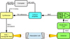 |
Fig. 1. Schematic of the general experimental setup. A single-pass setup is shown for the sake of clarity, although several measurements were performed with a double-pass setup, where the frequency source and detector are located on the same side of the cell. |
Measurement setups for  C(O)CH3.
The electromagnetic wave was frequency modulated (FM; f ≤ 50 kHz) with a 2f demodulation which causes Doppler limited absorption signals to appear close to a second derivative of a Gaussian. The modulation amplitude was ≤0.8 × HWHM. A 10 MHz rubidium atomic clock was used as a frequency standard. The accuracy of transition frequencies is mainly limited by standing waves, asymmetric line shapes also originating from nearby lines in a dense spectrum, and the linewidth which is dominated by Doppler-broadening. The uncertainty of a transition frequency Δf in a dense spectrum, such as that of acetone, usually increases for increasing frequencies since the Doppler width is proportional to the frequency of the electromagnetic wave. The uncertainties of transition frequencies were chosen to be Δf = HWHM/6.6; the value of 6.6 was determined as the average number of frequency steps needed to record one HWHM properly. A satisfactory signal-to-noise ratio (S/N) was typically achieved with 20 ms integration time per frequency step. To prevent systematic shifts in the frequency domain, we always averaged an upward scan and a downward scan (measuring a frequency window with increasing and decreasing frequencies, respectively).
We studied  C(O)CH3 using an isotopically enriched sample from Sigma-Aldrich with 99% 13C on the carbonyl C and a chemical purity of 99%. We recorded its spectrum at room temperature under static conditions, at a constant gas pressure of 5 μbar. We measured the main isotopolog of acetone, CH3C(O)CH3, and 13CH3C(O)CH3 with a pure sample of acetone in natural abundance. Because the relative natural abundance ratio is 87:2:1 for CH3C(O)CH3:13CH3C(O)CH3:
 C(O)CH3, we measured 13CH3C(O)CH in natural abundance in a constant gas flow at comparably high pressures up to 14 μbar. In order to increase the S/N further, the modulation amplitude was increased up to (1.0 − 1.5) × HWHM, and the total integration time per point was increased to 1.8 s.
3. Rotational spectroscopy of acetone
3.1. Spectroscopic properties of acetone
Acetone is a rather asymmetric oblate rotor with κ = (2B − A − C)/(A − C) = + 0.3720, which is quite far from the symmetric limit of +1. The symmetry of the rigid molecule is C2v, and the dipole moment component of 2.93 ± 0.03 D (Peter & Dreizler 1965) is along the b-inertial axis of the molecule. The selection rules are ΔJ = 0, ±1, ΔKa ≡ 1 mod(2), and ΔKc ≡ 1 mod(2).
The effective barrier to internal rotation of the two equivalent methyl rotors is moderately low, 251 cm−1, 361 K, or 3.00 kJ mol−1 (Groner 2000), such that most rotational transitions are split into four lines. These components are labeled by the quantum numbers of the internal rotation Hamiltonian of the two methyl groups in the absence of external electromagnetic fields, σ1 and σ2, respectively. Rotational transitions occur only within a given internal rotation component. Relative intensities for allowed b-type transitions can be derived by group-theory considerations and are listed in Table 2.
Relative intensities resulting from internal rotation of both methyl groups in acetone.
The two equivalent methyl rotors lead to two torsional modes whose fundamental frequencies are quite low in acetone; for the symmetric torsional mode v12 = 1 is at 77.8 cm−1 or 112 K (Kundu et al. 1992) while for the asymmetric torsional mode v17 = 1 is at 124.6 cm−1 or 179 K (Groner et al. 1987). Rotational transitions pertaining to these states are not much weaker than the ground state transitions at room temperature. This leads to a very rich rotational spectrum within a given vibrational state and a plethora of vibrational states that are stronger than the 13C isotopologs in natural isotopic composition.
Substitution of the carbonyl C atom by 13C, resulting in  C(O)CH3, retains the symmetry of the molecule. Moreover, the substitution has very small effects on the lower order spectroscopic parameters because the atom is close to the center of mass. In contrast, substitution of one methyl C atom by 13C, resulting in 13CH3C(O)CH3, lowers the symmetry and leads to changes even in the lower order spectroscopic parameters. This includes the internal rotation parameters associated with the two different rotors. However, the changes are small and may be neglected if the values are not determined with high accuracy. The number of internal rotation components is now five.
3.2. Spectroscopic analysis
We used the software package Assignment and Analysis of Broadband Spectra (AABS) developed by Z. Kisiel (Kisiel et al. 2005, 2012) for analyzing the experimental spectra. We employed an extended version of the “Effective Rotational HAMiltonian program for molecules with up to two periodic large-amplitude motions” (ERHAM) from P. Groner (Groner 1997; Groner et al. 2002) for modeling because we needed to fit large quantum numbers to experimental uncertainty efficiently. The extension allowed us to process more transitions and parameters from the input file and the Intel Fortran compiler partially optimized the program for parallel calculation.
The ERHAM code uses an effective rotational Hamiltonian for fitting one or two periodic large-amplitude motions (LAMs). It does not solve the internal-rotation Hamiltonian itself, in particular no barriers to internal rotation are calculated. The program uses the periodicity of eigenfunctions to expand them as a Fourier series. Its coefficient functions are dependent on the internal rotation variable. Furthermore, all matrix elements of the full Hamiltonian can be expanded as a Fourier series. The Hamiltonian H is of the form H = T + V, with T describing the kinetic energy and V describing the potential energy. Expressing overall rotation and internal rotation of two LAMs in a general form, T is
 (1)
(1)
with ω the overall angular velocity vector (3 × 1-matrix),  the velocities of both internal motions (2 × 1), Iω the moment of inertia of overall rotation (3 × 3), Iτ containing the moments of inertia of the internal motions on its diagonal (2 × 2), and Iωτ containing the cross terms (3 × 2).
The overall fitting procedure was as follows: after a round of new assignments, we carried out new fits with ERHAM under systematic variations of parameters to reach a weighted standard deviation close to 1.0, which means that the experimental data were fit within their uncertainties on average. Too many optimistic uncertainties, wrong assignments, or an incomplete or wrong model may cause values much larger than 1.0, whereas too many conservative uncertainties may lead to values smaller than 1.0. Transitions with large residuals after the fit (more than about ten times the uncertainties) were weighted out at this stage because of potential misassignments. Consequently, for each applicable combination of localized states of the first and second motions, labeled (q, q′), we tested possible missing parameters by including all parameters on the same order of n = K + P + R to the fit; K defines the order of PK, P of  , and R of
  . Next, sets of parameters with higher orders of n, as well as sets of parameters of ascending order of (q + q′), were added as long as the standard deviation improved by at least 10%. Subsequently, we searched for parameters which could be omitted from the fit without a significant increase in the weighted standard deviation of the fit. These were mostly parameters with large uncertainties compared to the magnitudes of their values. A new round of assignments was started after completion of this procedure until no new lines could be assigned in any of the spectral recordings.
At an advanced stage of the assignment process, we noticed that parameters with an odd order of n turned out to be indispensable. All parameters not in line with Watson’s A-reduction (Watson 1967) nor with the S-reduction (Winnewisser 1972; van Eijck 1974) are labeled in cylindrical tensor form with [BKPR]qq′ or ![Mathematical equation: $ [B^-_{KPR}]_{qq^{\prime}} $](/articles/aa/full_html/2019/09/aa35887-19/aa35887-19-eq18.gif) (the superscript − is to highlight that ω = −1) according to the tunneling parameter input summarized by Groner (2012) in Appendix A. Such parameters were used rarely in previous fits carried out with the ERHAM program. In addition, they also helped to obtain a greatly improved fit of the main isotopic species in its ground vibrational state.
(the superscript − is to highlight that ω = −1) according to the tunneling parameter input summarized by Groner (2012) in Appendix A. Such parameters were used rarely in previous fits carried out with the ERHAM program. In addition, they also helped to obtain a greatly improved fit of the main isotopic species in its ground vibrational state.
4. Results
4.1. Laboratory spectroscopy
We studied the ground vibrational states of the symmetric and asymmetric isotopologs  C(O)CH3 and 13CH3C(O)CH3, respectively. In addition, we investigated the ground as well as the first two torsionally excited states of the main isotopic species.
4.1.1. The symmetric isotopolog  C(O)CH3 in its ground vibrational state
Lovas & Groner (2006) determined 44 transition frequencies of 11 different rotational transitions with J ≤ 4 in the region of 10−25 GHz. The resulting spectroscopic parameters were accurate enough to assign low-J transitions up to 130 GHz. We were able to extend the assignments subsequently on the basis of improved predictions of the rotational spectrum to somewhat higher J and K quantum numbers, eventually reaching J = 92 and K = 45. Inclusion of the tunneling parameters [![Mathematical equation: $ [B^-_{010}]_{10} $](/articles/aa/full_html/2019/09/aa35887-19/aa35887-19-eq21.gif) (=[ga]10) and
(=[ga]10) and ![Mathematical equation: $ [B^-_{001}]_{10} $](/articles/aa/full_html/2019/09/aa35887-19/aa35887-19-eq22.gif) (= [gb]10) in the fit lowered the standard deviation by 17%. Our final line list consists of 5870 lines which were reproduced with a weighted standard deviation of 1.29 using 51 spectroscopic parameters, see Table 3.
(= [gb]10) in the fit lowered the standard deviation by 17%. Our final line list consists of 5870 lines which were reproduced with a weighted standard deviation of 1.29 using 51 spectroscopic parameters, see Table 3.

4.1.2. The asymmetric isotopolog 13CH3C(O)CH3 in its ground vibrational state
Lovas & Groner (2006) studied the same 11 rotational transitions with J ≤ 4 in the region of 10−25 GHz as they did for  C(O)CH3. The lower symmetry resulted in 55 transition frequencies, compared to 44 transitions for the symmetrically substituted isotopolog. The resulting spectroscopic parameters were again sufficiently accurate to search for transitions with low values of J. However, in the case of the asymmetrically substituted isotopolog, we did not have an isotopically enriched sample at our disposal. Nevertheless, we were able to identify a small number of unblended transitions of 13CH3C(O)CH3 in the acetone spectra recorded in natural isotopic composition. The assignments were beyond doubt because of our earlier investigation of an isotopically enriched sample. Transitions with Ka = 0 ← 1 and Ka = 1 ← 0 are particularly promising because they already overlap at fairly low J (oblate pairing). A typical fingerprint due to internal rotation for these partly collapsed transitions consists of three lines. In this case, transitions of the torsional substate with quantum numbers of (σ1 = 0, σ2 = 0) are observed as single lines (unblended), while lines of (±1, 0) and (0, ±1) are blended, as are (±1, ±1) and (±1, ∓1). This leads to an intensity ratio of 2 : (2 + 2):(1 + 1) = 1 : 2 : 1, see Table 2. This intensity ratio played a decisive role for assignments, as can be seen in Fig. 2.
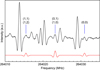 |
Fig. 2. Section of the rotational spectrum of acetone in natural isotopic composition (in black) in the region of the oblate paired |


As a first step, we recorded transitions in the frequency region 36−70 GHz and assigned transitions with J′←J″ = 6 ← 5 and 4 ← 3. After these assignments, we assigned transitions in higher frequency regions 81−130 GHz (setup 1b of Table 1 was used) and 244−351 GHz (setup 2a) for J′ ranging from 8 to 13 and 25 to 36, respectively. Relative intensities of candidate lines were compared to known unperturbed lines of the main isotopolog to ensure the assignments because the large number of lines in the spectral recordings frequently lead to blending.
The sextic centrifugal distortion parameters turned out to be insensitive to our dataset and were omitted from the final fit. In addition, we fixed [ΔJ]01 to its counterpart [ΔJ]10 and ϵ02 to ϵ20. The final fit had a weighted standard deviation of 0.93. The resulting spectroscopic parameters are given in Table 4.
4.1.3. The main isotopic species in its ground vibrational state
Groner et al. (2002) studied the main isotopolog quite extensively. However, striking discrepancies between the resulting predictions and our ALMA spectra of Sgr B2(N2), detailed in Sect. 4.2.1, motivated us to revisit the rotational spectroscopy of the main isotopolog. These discrepancies may be caused by the insufficient quantum number coverage of the experimental lines at higher J. The coverage is quite good for transitions without asymmetry splitting, that is transitions with high values of Ka (prolate paired) or Kc (oblate paired), respectively, even though some of the prolate paired transitions did not fit well (Groner et al. 2002). Transitions with asymmetry splitting are largely missing for higher quantum numbers. They are weaker by a factor of two and frequently display a more complex internal rotation pattern. Another reason may well be that the weighted standard deviation of their fit, 1.58, is only close to the experimental uncertainty.
We tested parameters with ω = − 1 to improve the quality of the fit, analogously to our  C(O)CH3 fit. With just two added parameters, six other parameters could be omitted and the weighted standard deviation of the same dataset still improved to 1.29. In the fits of Groner et al. (2002) and our modified fit of Groner et al. (2002) (see second and third column of Table 5, respectively), all transitions were treated as single lines even if they had the same frequency since the 2002 version of ERHAM used by Groner et al. (2002) did not properly account for blended lines.
The ERHAM version available nowadays, as our extended version, is capable of properly treating blended lines. This frequently leads to lower weighted standard deviations. We achieved a more decisive improvement of our model by assigning more than 1000 transitions of the main isotopolog in the frequency regions of 36−70 GHz and 82−125 GHz. This extension proved to be sufficient for our astronomical observations which cover a considerable part of the second frequency region. A comparison of the parameters derived by Groner et al. (2002), the refitted version of their data, and the final parameter values derived in this work can be found in Table 5. A comparison of low-order spectroscopic parameters of the three isotopic species of acetone is given in Table 6.

4.1.4. The main isotopic species in its first two torsionally excited states
Clear indications in the astronomical emission spectra of two torsionally excited states of the main species, v12 = 1 and v17 = 1, made it indispensable to extend the line lists to ensure clear identification of lines within them. Fitting and modeling the first two torsionally excited states was considerably more challenging. For both states, the overall aim in modeling the spectra was to derive models that fit our data close to experimental uncertainty to simply allow for astronomical detection of these species. Nevertheless, the initial line lists for v12 = 1 and v17 = 1, consisting of around 400 and 600 lines from Groner et al. (2006, 2008), respectively, were extended by almost 1300 and more than 600 lines, respectively.
Attempts to improve the fits of the two excited torsional states of the main isotopic species were only partially successful, the weighted standard deviation values were 1.36 and 1.62 for v12 = 1 and v17 = 1, respectively. Therefore, only selected parameters of these states are listed and compared to values of the ground vibrational state of acetone-12C in Table 7. The full list of parameters can be found in Tables A.1 and A.2, for v12 = 1 and v17 = 1, respectively.
4.2. Radioastronomical observations
We used the EMoCA spectral line survey performed toward the high-mass star forming region Sagittarius B2(N) with ALMA to search for the 13C isotopologs of acetone and for transitions of the 12C isotopolog in its torsionally excited states v12 = 1 and v17 = 1. Details about the observations, data reduction, and the method used to identify the detected lines and derive column densities can be found in Belloche et al. (2016). In short, the survey covers the frequency range from 84.1 GHz to 114.4 GHz with a spectral resolution of 488.3 kHz (1.7 to 1.3 km s−1). It was performed with five frequency tunings called S1–S5. The median angular resolution is 1.6″. In this work we focus on the peak position of the hot molecular core Sgr B2(N2) with J2000 equatorial coordinates ( ,
,  ).
).
4.2.1. CH3C(O)CH3
Before searching for transitions of the 13C isotopologs of acetone, we first modeled the emission of the main isotopolog in the EMoCA survey of Sgr B2(N2). As described in Belloche et al. (2016), we proceeded in an iterative way using Weeds (Maret et al. 2011) under the local thermodynamic equilibrium (LTE) approximation. Each species was modeled with the following five free parameters: size of the emission region, rotational temperature, column density, line width, and velocity offset with respect to the systemic velocity of the source. We modeled the emission of acetone on top of the contribution of all the molecules we already identified so far in this survey. This allowed us to spot 26 spectral lines of acetone that are not contaminated by the emission of other species. We used these transitions to fit the size of the acetone emission in the interferometric maps toward Sgr B2(N2). We derived a median size (FWHM) of 1.2″. The line width and velocity offset were derived directly from these uncontaminated transitions.
With these parameters and a first guess of the rotational temperature, we computed synthetic spectra for v = 0, v12 = 1, and v17 = 1, which allowed us to identify rotational transitions of both torsionally excited states in the EMoCA spectrum of Sgr B2(N2). We used all the transitions of these states and the vibrational ground state that were not contaminated too much by other species to build a population diagram. This diagram is shown in Fig. 3. It contains 110, 40, and 17 spectral lines of v = 0, v12 = 1, and v17 = 1, respectively. Figure 3b shows the population diagram after correcting the integrated intensities for the line optical depth and contamination due to the other identified species that are included in our full model. A fit to this diagram yields a rotational temperature of 152 ± 4 K. This temperature is a fair indication of the true rotational temperature of the molecule. However, its uncertainty is likely underestimated because the dispersion of the datapoints in Fig. 3b is dominated by residual contamination from unidentified species while the errors reported on the individual datapoints and used for the weighted fit are purely statistical. For comparison purposes, a fit limited to the transitions in the vibrational ground state only yields a temperature of 147 ± 5 K. In the following, we used a temperature of 140 K, which is still close to the fitted value, to model the spectrum of acetone.
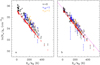 |
Fig. 3. Population diagram of CH3C(O)CH3 toward Sgr B2(N2). The observed datapoints are shown in black, blue, and orange for the v = 0, v12 = 1, and v17 = 1 states, respectively, while the synthetic populations are shown in red. No correction is applied in panel a. In panel b, the optical depth correction was applied to both the observed and synthetic populations and the contamination by all other species included in the full model was removed from the observed datapoints. The purple line is a linear fit to the observed populations (in linear-logarithmic space). |
The last parameter to adjust is the column density. We obtained a value of 4 × 1017 cm−2 by fitting the observed spectrum (see Table 8). The best-fit synthetic spectra of v = 0, v12 = 1, and v17 = 1 are overlaid on the EMoCA spectrum of Sgr B2(N2) in Figs. B.1–B.3, respectively. We also display the full model that contains the contributions of all species identified so far. We counted 122, 33, and 13 transitions or groups of transitions of acetone that are clearly detected in its vibrational ground state v = 0 and its torsionally excited states v12 = 1 and v17 = 1, respectively, with little contamination from other species.
Parameters of our best-fit LTE model of acetone and its 13C isotopologs toward Sgr B2(N2).
4.2.2. 13CH3C(O)CH3 and  C(O)CH3
We used the parameters derived for the main isotopolog of acetone to search for transitions of the 13C-substituted isotopologs 13CH3C(O)CH3 and  C(O)CH3. On the one hand, we find tentative evidence for the presence of 13CH3C(O)CH3 in Sgr B2(N2). The transitions covered by our survey are shown in Fig. B.4. Only one transition (at 110.131 GHz) is clearly detected with little contamination from other species, but several transitions contribute significantly to the detected signal as well. The discrepancy at 108.025 GHz is at the 2σ level, so it is probably not significant. It may be due to a slight overestimate of the baseline level. The synthetic spectrum shown in Fig. B.4 was computed with a column density of 3.0 × 1016 cm−2 (see Table 8), which is 13 times lower than the column density of the main isotopolog. Accounting for the fact that 13CH3C(O)CH3 contains two equivalent methyl groups, this yields a 12C/13C isotopic ratio of 27 for acetone, which is in agreement with the isotopic ratio derived for methanol and ethanol in this source (25, see Müller et al. 2016a). This gives us confidence that the assignment of the transition at 110.131 GHz to 13CH3C(O)CH3 is robust.
On the other hand, we did not detect any transition from  C(O)CH3. In Fig. B.5, we show a synthetic spectrum computed with a column density of 1.5 × 1016 cm−2, that is half of the column density of 13CH3C(O)CH3 as expected if the two species are drawn from the same parent 12C/13C isotopic ratio. Fractionation of 13C may lead to a different column density as discussed in Koerber et al. (2013) for the case of dimethyl ether. However, so far, we have no indications of 13C fractionation of complex organic molecules in Sgr B2(N2), see also Belloche et al. (2016) and Müller et al. (2016a). The synthetic spectrum is consistent with the observed one, suggesting that this isotopolog may be present in Sgr B2(N2) at this column density level. However, we can not exclude a higher or lower column density level and given that no single transition is individually detected, we report a nondetection in Table 8.
5. Discussion
5.1. Laboratory spectroscopy
We were able to extend the experimental line list of  C(O)CH3 thanks to an isotopically enriched sample. The high values of J and K of up to 92 and 45, respectively, ensure that observations of this symmetric isotopolog in its ground vibrational state are not limited by laboratory spectroscopy. In comparison, Groner et al. (2002) assigned lines of the main isotopolog CH3C(O)CH3 up to J = 60.
An isotopically enriched sample for 13CH3C(O)CH3 is not yet available. Therefore, our improvements were more modest for this isotopolog. Nevertheless, the data were sufficient to identify this species in our ALMA data tentatively.
We doubled the number of assigned transitions of the main isotopolog over the course of our investigations and obtained a greatly improved spectroscopic parameter set that reproduced our astronomical observations well. One explanation in comparison to the model of Groner et al. (2002) may be that transitions of complex molecules need extensive quantum number coverage in the assignments that is preferably over the full frequency range for proper modeling. This was also observed by some of the co-authors in the case of propanal (Zingsheim et al. 2017).
As mentioned in Sect. 3.1, substitution of the carbonyl-C by 13C retains the symmetry. In addition, Table 6 demonstrates that the low-order spectroscopic parameters are, in fact, very similar to those of the main isotopolog. This is expected because of the proximity of the carbonyl-C to the center of mass of the molecule. The asymmetrically substituted 13C isotopolog displays pronounced differences in the rotational and quartic centrifugal distortion parameters. The tunneling parameters differ slightly, and the averages for the two rotors are usually quite close to the values of the other two isotopologs; somewhat larger deviations are probably caused by the experimental line list that is still fairly small.
Progress on the torsionally excited states of CH3C(O)CH3 was not entirely satisfactorily despite the greatly extended line lists. Nevertheless, the spectroscopic parameters were sufficient for assignment of transitions within these excited states in our astronomical data. However, striking deviations occur between some observed and calculated transition frequencies, suggesting that these models are still not satisfactory. This is reflected in the weighted standard deviations of the fits of 1.36 and 1.62, respectively, and by the uncommon selection and quite large number of spectroscopic parameters, see Tables A.1 and A.2. Ilyushin & Hougen (2013) explained the failure of ERHAM to fit the excited torsional states of acetone satisfactorily by the amount of torsion-torsion interaction that is not modeled in single state fits. These interactions are treated satisfactorily in the PAM_C2v_2tops program (Ilyushin & Hougen 2013). Armieieva et al. (2016) fit 12128 microwave and 7 FIR line frequencies in a joined fit of v = 0, v12 = 1, and v17 = 1 of CH3C(O)CH3 with a reasonable number of 99 parameters to a root-mean-square deviation of merely 0.78, highlighting the advantages of including torsion-torsion interactions.
5.2. Radioastronomical observations
The new spectroscopic predictions produced over the course of this work yield much better agreement with the ALMA spectrum than what could previously be achieved with the predictions available in the JPL catalog (Pickett et al. 1998), which were contributed by B. J. Drouin in 2008 by recalculating the data from Groner et al. (2002) and references therein. Figure 4 compares the synthetic spectra computed with the same LTE parameters for the vibrational ground state in both cases for four selected frequency ranges. While prominent discrepancies were present between the JPL predictions and the observed spectrum, for instance at 87.820 GHz, 87.824 GHz, or 91.592 GHz, the synthetic spectrum produced with the new predictions agrees perfectly well with the observed spectrum. This confirms that the new predictions of the vibrational ground state of acetone are more reliable, at least in the 3 mm wavelength range.
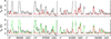 |
Fig. 4. Examples of lines of acetone covered by EMoCA toward Sgr B2(N2). The ALMA spectrum is shown in black in all panels. The red spectrum shows the synthetic spectrum of acetone computed with the JPL entry (tag 58003, version 1) in the top row and with the new predictions presented in this work in the bottom row. The synthetic spectrum of all molecules identified so far, including acetone, is shown in green. The central frequency and width of the frequency range (in parentheses) are indicated at the bottom in MHz. The angular resolution (HPBW) is also indicated. The y-axis is labeled in brightness temperature units. The dotted line indicates the 3σ noise level. The new predictions match the observed spectrum much better. |
The agreement between the synthetic spectra of v12 = 1 and v17 = 1 with the EMoCA spectrum of Sgr B2(N2) is good (see Figs. B.2 and B.3). Still, we notice discrepancies larger than 3σ and smaller than ∼5σ at the following few frequencies: 93.254 GHz, 98.489 GHz, 103.828 GHz, and 108.857 GHz for v12 = 1, and 95.464 GHz and 111.541 GHz for v17 = 1. Possible reasons for these discrepancies are inaccuracies of the predicted frequencies of acetone (e.g., at 93.254 GHz, 98.489 GHz, 103.828 GHz, and 95.464 GHz with formal uncertainties of the predictions larger than 100 kHz), uncertainties as to the true level of the baseline, and inaccuracies of the predicted frequencies of contaminating species in the cases where the discrepancy does not directly arise from the acetone spectrum but from the full model. All in all, these small discrepancies that may be solved with higher-accuracy predictions, as mentioned in Sect. 4.1.4 and discussed in Sect. 5.1, do not affect the reliability of our identifications of both torsionally excited states.
6. Conclusion
The main isotopic species of acetone, CH3C(O)CH3, and  C(O)CH3 are described by robust models, allowing for proper modeling of these species in astronomical sources. The predicted transition frequencies by our derived models for
  C(O)CH3 and CH3C(O)CH3 are reliable into the terahertz region. Therefore, these models can be of high interest for the analyses of hot-core and hot-corino surveys performed with ALMA in all its bands. We intend to revisit the spectrum of 13CH3C(O)CH3 with an enriched sample. The model derived for 13CH3C(O)CH3 with a standard deviation of 0.93 is a good and robust cornerstone for continuing the study of this species in the millimeter- and submillimeter-wavelength region in the future. Predictions of transitions involving quantum numbers where J = Kc may be reliable up to 500 GHz or J ≈ 50. Transition frequencies with lower Kc should be viewed with increased caution. Thus far, the vibrational ground states of these three isotopologs can be treated as isolated states.
On the other hand, the developer of ERHAM, P. Groner and his co-authors stated in a recent paper “that the ERHAM code is unable to fit the v17 = 1 state of acetone without accounting for the interactions with other vibrational states” (Morina et al. 2019) as was explained by Ilyushin & Hougen (2013). The same conclusion may be drawn by looking at the results of this work for the vibrationally excited states v12 = 1 and v17 = 1. Modeling of these states requires including interactions between different vibrational states. A more robust model for the torsionally excited states is derived by Armieieva et al. (2016) using the PAM_C2v_2tops program (Ilyushin & Hougen 2013). This simultaneously fits the ground state and both torsionally excited states; however, no linelist is publicly available. Such an approach may also be applied beneficially to the torsionally excited states of the 13C-species in the future. It is especially important to note that for the symmetric isotopolog  C(O)CH3, transition frequencies of excited states with a symmetric motion around the symmetry axis of the molecule are only marginally shifted compared to the main species. This occurs because the replaced carbon atom lies on this symmetry axis, which coincides with the observable rotation of the molecule around the b-axis.
Predictions of the ground state rotational spectra of the three isotopic species of acetone in the study will be available in the catalog section of the CDMS2 (Endres et al. 2016). All fit files and auxiliary files will be available in the data section of the CDMS3.
See, e. g., the Molecules in Space page, https://cdms.astro.uni-koeln.de/classic/molecules, of the Cologne Database for Molecular Spectroscopy, CDMS.
Acknowledgments
M.H.O. and O.Z. are very thankful to Peter Groner for various comments and recommendations for using his ERHAM program. This paper makes use of the following ALMA data: ADS/JAO.ALMA#2011.0.00017.S, ADS/JAO.ALMA#2012.1.00012.S. ALMA is a partnership of ESO (representing its member states), NSF (USA) and NINS (Japan), together with NRC (Canada), NSC and ASIAA (Taiwan), and KASI (Republic of Korea), in cooperation with the Republic of Chile. The Joint ALMA Observatory is operated by ESO, AUI/NRAO, and NAOJ. The interferometric data are available in the ALMA archive at https://almascience.eso.org/aq/. This work is supported by the Collaborative Research Centre 956, sub-project B3, funded by the Deutsche Forschungsgemeinschaft (DFG) – project ID 184018867. Our research benefited from NASA’s Astrophysics Data System (ADS).
References
- Armieieva, I. A., Ilyushin, V. V., Alekseev, E. A., et al. 2016, Russ. Radio Phys. Radio Astron., 21, 37 [NASA ADS] [CrossRef] [Google Scholar]
- Belloche, A., Menten, K. M., Comito, C., et al. 2008, A&A, 482, 179 [NASA ADS] [CrossRef] [EDP Sciences] [Google Scholar]
- Belloche, A., Garrod, R. T., Müller, H. S. P., et al. 2009, A&A, 499, 215 [NASA ADS] [CrossRef] [EDP Sciences] [Google Scholar]
- Belloche, A., Müller, H. S. P., Menten, K. M., et al. 2013, A&A, 559, A47 [NASA ADS] [CrossRef] [EDP Sciences] [Google Scholar]
- Belloche, A., Garrod, R. T., Müller, H. S. P., & Menten, K. M. 2014, Science, 345, 1584 [NASA ADS] [CrossRef] [PubMed] [Google Scholar]
- Belloche, A., Müller, H. S. P., Garrod, R. T., & Menten, K. M. 2016, A&A, 587, A91 [NASA ADS] [CrossRef] [EDP Sciences] [Google Scholar]
- Bouchez, A., Walters, A., Müller, H. S. P., et al. 2012, J. Quant. Spectr. Rad. Transf., 113, 1148 [NASA ADS] [CrossRef] [Google Scholar]
- Carvajal, M., Margulès, L., Tercero, B., et al. 2009, A&A, 500, 1109 [NASA ADS] [CrossRef] [EDP Sciences] [Google Scholar]
- Combes, F., Gerin, M., Wootten, A., et al. 1987, A&A, 180, L13 [NASA ADS] [Google Scholar]
- Demyk, K., Mäder, H., Tercero, B., et al. 2007, A&A, 466, 255 [NASA ADS] [CrossRef] [EDP Sciences] [Google Scholar]
- Endres, C. P., Lewen, F., Giesen, T. F., et al. 2007, Rev. Sci. Instrum., 78, 043106 [NASA ADS] [CrossRef] [Google Scholar]
- Endres, C. P., Drouin, B. J., Pearson, J. C., et al. 2009, A&A, 504, 635 [NASA ADS] [CrossRef] [EDP Sciences] [Google Scholar]
- Endres, C. P., Schlemmer, S., Schilke, P., Stutzki, J., & Müller, H. S. P. 2016, J. Mol. Spectrosc., 327, 95 [Google Scholar]
- Friedel, D. N., Snyder, L. E., Remijan, A. J., & Turner, B. E. 2005, ApJ, 632, L95 [NASA ADS] [CrossRef] [Google Scholar]
- Groner, P. 1997, J. Chem. Phys., 107, 4483 [NASA ADS] [CrossRef] [Google Scholar]
- Groner, P. 2000, J. Mol. Struct., 550, 473 [NASA ADS] [CrossRef] [Google Scholar]
- Groner, P. 2012, J. Mol. Spectrosc., 278, 52 [NASA ADS] [CrossRef] [Google Scholar]
- Groner, P., Guirgis, G. A., & Durig, J. R. 1987, J. Chem. Phys., 86, 565 [NASA ADS] [CrossRef] [Google Scholar]
- Groner, P. J. M., Albert, S., Herbst, E., et al. 2002, ApJS, 142, 145 [NASA ADS] [CrossRef] [Google Scholar]
- Groner, P., Herbst, E., De Lucia, F. C., et al. 2006, J. Mol. Struct., 795, 173 [NASA ADS] [CrossRef] [Google Scholar]
- Groner, P., Medvedev, I. R., De Lucia, F. C., & Drouin, B. J. 2008, J. Mol. Spectrosc., 251, 180 [NASA ADS] [CrossRef] [Google Scholar]
- Guarnieri, A., & Huckauf, A. 2003, Z. Naturforsch. A, 58, 275 [NASA ADS] [CrossRef] [Google Scholar]
- Haykal, I., Motiyenko, R. A., Margulès, L., & Huet, T. R. 2013, A&A, 549, A96 [NASA ADS] [CrossRef] [EDP Sciences] [Google Scholar]
- Ilyushin, V. V., & Hougen, J. T. 2013, J. Mol. Spectrosc., 289, 41 [NASA ADS] [CrossRef] [Google Scholar]
- Jørgensen, J. K., van der Wiel, M. H. D., Coutens, A., et al. 2016, A&A, 595, A117 [NASA ADS] [CrossRef] [EDP Sciences] [Google Scholar]
- Jørgensen, J. K., Müller, H. S. P., Calcutt, H., et al. 2018, A&A, 620, A170 [NASA ADS] [CrossRef] [EDP Sciences] [Google Scholar]
- Kisiel, Z., Pszczółkowski, L., Medvedev, I. R., et al. 2005, J. Mol. Spectrosc., 233, 231 [Google Scholar]
- Kisiel, Z., Pszczółkowski, L., Drouin, B. J., et al. 2012, J. Mol. Spectrosc., 280, 134 [NASA ADS] [CrossRef] [Google Scholar]
- Koerber, M., Bisschop, S. E., Endres, C. P., et al. 2013, A&A, 558, A112 [NASA ADS] [CrossRef] [EDP Sciences] [Google Scholar]
- Kundu, T., Thakur, S. N., & Goodman, L. 1992, J. Chem. Phys., 97, 5410 [NASA ADS] [CrossRef] [Google Scholar]
- Lattanzi, V., Walters, A., Drouin, B. J., & Pearson, J. C. 2008, ApJS, 176, 536 [NASA ADS] [CrossRef] [Google Scholar]
- Lewen, F., & Gendriesch, R. 1998, Rev. Sci. Instrum., 69, 32 [NASA ADS] [CrossRef] [Google Scholar]
- Lovas, F. J., & Groner, P. 2006, J. Mol. Spectrosc., 236, 173 [NASA ADS] [CrossRef] [Google Scholar]
- Lykke, J. M., Coutens, A., Jørgensen, J. K., et al. 2017, A&A, 597, A53 [NASA ADS] [CrossRef] [EDP Sciences] [Google Scholar]
- Maret, S., Hily-Blant, P., Pety, J., et al. 2011, A&A, 526, A47 [NASA ADS] [CrossRef] [EDP Sciences] [Google Scholar]
- Margulès, L., Motiyenko, R. A., Ilyushin, V. V., & Guillemin, J. C. 2015, A&A, 579, A46 [NASA ADS] [CrossRef] [EDP Sciences] [Google Scholar]
- Margulès, L., Belloche, A., Müller, H. S. P., et al. 2016, A&A, 590, A93 [NASA ADS] [CrossRef] [EDP Sciences] [Google Scholar]
- Morina, L., Obst, S., Unrath, M., et al. 2019, J. Mol. Spectrosc., 356, 1 [Google Scholar]
- Müller, H. S. P., Belloche, A., Menten, K. M., et al. 2008, J. Mol. Spectrosc., 251, 319 [CrossRef] [Google Scholar]
- Müller, H. S. P., Drouin, B. J., & Pearson, J. C. 2009, A&A, 506, 1487 [NASA ADS] [CrossRef] [EDP Sciences] [Google Scholar]
- Müller, H. S. P., Belloche, A., Xu, L.-H., et al. 2016a, A&A, 587, A92 [NASA ADS] [CrossRef] [EDP Sciences] [Google Scholar]
- Müller, H. S. P., Walters, A., Wehres, N., et al. 2016b, A&A, 595, A87 [NASA ADS] [CrossRef] [EDP Sciences] [Google Scholar]
- Peter, R., & Dreizler, H. 1965, Z. Naturforsch., 20a, 301 [Google Scholar]
- Pickett, H. M., Poynter, R. L., Cohen, E. A., et al. 1998, J. Quant. Spectr. Rad. Transf., 60, 883 [NASA ADS] [CrossRef] [Google Scholar]
- Snyder, L. E., Lovas, F. J., Mehringer, D. M., et al. 2002, ApJ, 578, 245 [NASA ADS] [CrossRef] [Google Scholar]
- Swalen, J. D., & Costain, C. C. 1959, J. Chem. Phys., 31, 1562 [NASA ADS] [CrossRef] [Google Scholar]
- van Eijck, B. P. 1974, J. Mol. Spectrosc., 53, 246 [NASA ADS] [CrossRef] [Google Scholar]
- Watson, J. K. G. 1967, J. Chem. Phys., 46, 1935 [NASA ADS] [CrossRef] [Google Scholar]
- Winnewisser, G. 1972, J. Chem. Phys., 56, 2944 [NASA ADS] [CrossRef] [Google Scholar]
- Zingsheim, O., Müller, H. S. P., Lewen, F., et al. 2017, J. Mol. Spectrosc., 342, 125 [NASA ADS] [CrossRef] [Google Scholar]
Appendix A: Complementary spectroscopic parameters
Tables A.1 and A.2 show the full list of spectroscopic parameters of υ12 = 1 and υ17 = 1 of CH3C(O)CH3, respectively. A selection of these parameters is listed in Table 7 and compared to the ground vibrational state of CH3C(O)CH3. The derived models for the vibrationally excited states should be viewed with caution.
Spectroscopic parameters(a) of the vibrationally excited state υ12 = 1 of CH3C(O)CH3.
Spectroscopic parameters(a) of the vibrationally excited state υ17 = 1 of CH3C(O)CH3.
Appendix B: Complementary figures
Figures B.1–B.5 show the transitions of CH3C(O)CH3v = 0, v12 = 1, and v17 = 1, as well as 13CH3C(O)CH3v = 0 and CH3 13C(O)CH3v = 0 that are covered by the EMoCA survey and contribute significantly to the signal detected toward Sgr B2(N2).
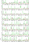 |
Fig. B.1. Transitions of CH3C(O)CH3v = 0 covered by the EMoCA survey. The best-fit LTE synthetic spectrum of CH3C(O)CH3v = 0 is displayed in red and overlaid on the observed spectrum of Sgr B2(N2) shown in black. The green synthetic spectrum contains the contributions of all molecules identified in our survey so far, including the species shown in red. The central frequency and width of the frequency range (in parentheses) are indicated in MHz below each panel. The angular resolution (HPBW) is also indicated. The y-axis is labeled in brightness temperature units. The dotted line indicates the 3σ noise level. |
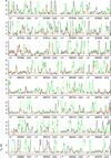 |
Fig. B.1. continued. |
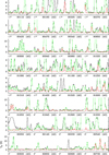 |
Fig. B.1. continued. |
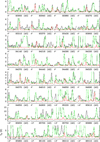 |
Fig. B.1. continued. |
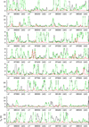 |
Fig. B.1. continued. |
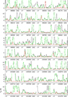 |
Fig. B.1. continued. |
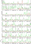 |
Fig. B.1. continued. |
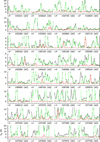 |
Fig. B.1. continued. |
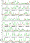 |
Fig. B.1. continued. |
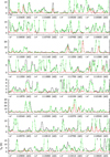 |
Fig. B.1. continued. |
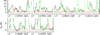 |
Fig. B.1. continued. |
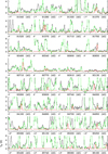 |
Fig. B.2. continued. |
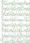 |
Fig. B.2. continued. |
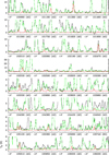 |
Fig. B.2. continued. |
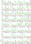 |
Fig. B.2. continued. |
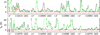 |
Fig. B.2. continued. |
2
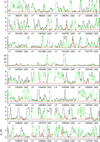 |
Fig. B.3. continued. |
2
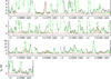 |
Fig. B.3. continued. |

All Tables
Relative intensities resulting from internal rotation of both methyl groups in acetone.
Parameters of our best-fit LTE model of acetone and its 13C isotopologs toward Sgr B2(N2).
Spectroscopic parameters(a) of the vibrationally excited state υ12 = 1 of CH3C(O)CH3.
Spectroscopic parameters(a) of the vibrationally excited state υ17 = 1 of CH3C(O)CH3.
All Figures
|
Fig. 1. Schematic of the general experimental setup. A single-pass setup is shown for the sake of clarity, although several measurements were performed with a double-pass setup, where the frequency source and detector are located on the same side of the cell. |
| In the text | |
|
Fig. 2. Section of the rotational spectrum of acetone in natural isotopic composition (in black) in the region of the oblate paired |
| In the text | |
|
Fig. 3. Population diagram of CH3C(O)CH3 toward Sgr B2(N2). The observed datapoints are shown in black, blue, and orange for the v = 0, v12 = 1, and v17 = 1 states, respectively, while the synthetic populations are shown in red. No correction is applied in panel a. In panel b, the optical depth correction was applied to both the observed and synthetic populations and the contamination by all other species included in the full model was removed from the observed datapoints. The purple line is a linear fit to the observed populations (in linear-logarithmic space). |
| In the text | |
|
Fig. 4. Examples of lines of acetone covered by EMoCA toward Sgr B2(N2). The ALMA spectrum is shown in black in all panels. The red spectrum shows the synthetic spectrum of acetone computed with the JPL entry (tag 58003, version 1) in the top row and with the new predictions presented in this work in the bottom row. The synthetic spectrum of all molecules identified so far, including acetone, is shown in green. The central frequency and width of the frequency range (in parentheses) are indicated at the bottom in MHz. The angular resolution (HPBW) is also indicated. The y-axis is labeled in brightness temperature units. The dotted line indicates the 3σ noise level. The new predictions match the observed spectrum much better. |
| In the text | |
|
Fig. B.1. Transitions of CH3C(O)CH3v = 0 covered by the EMoCA survey. The best-fit LTE synthetic spectrum of CH3C(O)CH3v = 0 is displayed in red and overlaid on the observed spectrum of Sgr B2(N2) shown in black. The green synthetic spectrum contains the contributions of all molecules identified in our survey so far, including the species shown in red. The central frequency and width of the frequency range (in parentheses) are indicated in MHz below each panel. The angular resolution (HPBW) is also indicated. The y-axis is labeled in brightness temperature units. The dotted line indicates the 3σ noise level. |
| In the text | |
|
Fig. B.1. continued. |
| In the text | |
|
Fig. B.1. continued. |
| In the text | |
|
Fig. B.1. continued. |
| In the text | |
|
Fig. B.1. continued. |
| In the text | |
|
Fig. B.1. continued. |
| In the text | |
|
Fig. B.1. continued. |
| In the text | |
|
Fig. B.1. continued. |
| In the text | |
|
Fig. B.1. continued. |
| In the text | |
|
Fig. B.1. continued. |
| In the text | |
|
Fig. B.1. continued. |
| In the text | |
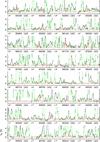 |
Fig. B.2. Same as Fig. B.1, but for CH3C(O)CH3v12 = 1. |
| In the text | |
|
Fig. B.2. continued. |
| In the text | |
|
Fig. B.2. continued. |
| In the text | |
|
Fig. B.2. continued. |
| In the text | |
|
Fig. B.2. continued. |
| In the text | |
|
Fig. B.2. continued. |
| In the text | |
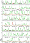 |
Fig. B.3. Same as Fig. B.1, but for CH3C(O)CH3v17 = 1. |
| In the text | |
|
Fig. B.3. continued. |
| In the text | |
|
Fig. B.3. continued. |
| In the text | |
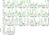 |
Fig. B.4. Same as Fig. B.1, but for 13CH3C(O)CH3v = 0. |
| In the text | |
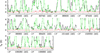 |
Fig. B.5. Same as Fig. B.1, but for |
| In the text | |
Current usage metrics show cumulative count of Article Views (full-text article views including HTML views, PDF and ePub downloads, according to the available data) and Abstracts Views on Vision4Press platform.
Data correspond to usage on the plateform after 2015. The current usage metrics is available 48-96 hours after online publication and is updated daily on week days.
Initial download of the metrics may take a while.