| Issue |
A&A
Volume 629, September 2019
|
|
|---|---|---|
| Article Number | A20 | |
| Number of page(s) | 13 | |
| Section | The Sun | |
| DOI | https://doi.org/10.1051/0004-6361/201935850 | |
| Published online | 27 August 2019 | |
Fundamental transverse vibrations of the active region solar corona⋆
1
Instituto de Astrofísica de Canarias, 38205 La Laguna, Tenerife, Spain
e-mail: This email address is being protected from spambots. You need JavaScript enabled to view it.
2
Departamento de Astrofísica, Universidad de La Laguna, 38206 La Laguna, Tenerife, Spain
3
Departament Física, Universitat de les Illes Balears, 07122 Palma de Mallorca, Spain
4
Institute of Applied Computing & Community Code (IAC 3), UIB, Spain
5
University of St Andrews, St Andrews KY16 9AJ, UK
Received:
7
May
2019
Accepted:
9
July
2019
Abstract
Context. Some high-resolution observations have revealed that the active region solar corona is filled with a myriad of thin strands even in apparently uniform regions with no resolved loops. This fine structure can host collective oscillations involving a large portion of the corona due to the coupling of the motions of the neighbouring strands.
Aims. We study these vibrations and the possible observational effects.
Methods. We theoretically investigated the collective oscillations inherent to the fine structure of the corona. We have called them fundamental vibrations because they cannot exist in a uniform medium. We used the T-matrix technique to find the normal modes of random arrangements of parallel strands. We considered an increasing number of tubes to understand the vibrations of a huge number of tubes of a large portion of the corona. We additionally generated synthetic time-distance Doppler and line-broadening diagrams of the vibrations of a coronal region to compare with observations.
Results. We have found that the fundamental vibrations are in the form of clusters of tubes where not all the tubes participate in the collective mode. The periods are distributed over a wide band of values. The width of the band increases with the number of strands but rapidly reaches an approximately constant value. We have found an analytic approximate expression for the minimum and maximum periods of the band. The frequency band associated with the fine structure of the corona depends on the minimum separation between strands. We have found that the coupling between the strands is on a large extent and the motion of one strand is influenced by the motions of distant tubes. The synthetic Dopplergrams and line-broadening maps show signatures of collective vibrations, not present in the case of purely random individual kink vibrations.
Conclusions. We conclude that the fundamental vibrations of the corona can contribute to the energy budget of the corona and they may have an observational signature.
Key words: Sun: corona / Sun: oscillations
A movie associated to Fig. 10 is available at https://www.aanda.org
© ESO 2019
1. Introduction and motivation
Early X-ray and extreme ultra-violet (EUV) observations by rocket-borne instruments (Vaiana et al. 1968; van Speybroeck et al. 1970) and onboard Skylab (Tousey et al. 1973; Vaiana et al. 1973) revealed that the active region (AR) corona is formed of a myriad of coronal loops. Because of the high anisotropy of the solar corona, and in particular that of transport coefficients whose parallel components to the field are much larger than their perpendicular components, it is thought that field-aligned structures should evolve largely independently on a given timescale (Klimchuk 2015). This suggests the existence of coronal strands, that is, elemental flux tubes, as the building blocks of coronal loops and the entire solar corona. This concept has received support either directly from some recent high-resolution observations, or indirectly from the combination of observations and modelling. Indeed, several works using Atmospheric Imaging Assembly (AIA) from the Solar Dynamics Observatory (Lemen et al. 2011), Extreme-Ultraviolet Imaging Spectrometer (EIS) from Hinode (Tsuneta et al. 2008), High Resolution Coronal Imager (Hi-C; Cirtain et al. 2013), and Interface Region Imaging Spectrograph (IRIS; de Pontieu et al. 2014) have found strand sizes of a few hundred kilometres (see e.g. Peter et al. 2013; Brooks et al. 2012, 2013, 2016). Antolin & Rouppe van der Voort (2012) observed strand-like structures of a few hundred kilometres in observations of coronal rain with the CRisp Imaging SpectroPolarimeter (CRISP) of the Swedish Solar Telescope (Scharmer et al. 2008) instrument. Antolin et al. (2015) have shown that the distribution of rain strands peaks at about 200 km and falls abruptly at the resolution limit, suggesting that even lower sizes are present (see also Scullion et al. 2014). This tip of the iceberg distribution is further supported by observations of flare-driven rain at even higher resolution with the New Solar Telescope (NST) of Big Bear Solar Observatory (Jing et al. 2016), in which the distribution peaks at 120 km with again a sharp cut-off at smaller sizes. Some authors claim that strands have radii as small as a few tens of kilometres (Peter et al. 2013). Hence, it is possible that coronal loops and more generally the corona are structured in the form of a myriad of thin flux tubes called strands.
The volumetric filling factor, f = Vs/V, measures the portion of a coronal region volume, V, filled with strands with a total volume Vs. The filling factor can be estimated using spectroscopic observations. Warren et al. (2008) found volumetric filling factors of 10% in AR loops. The authors also found a very narrow band of temperatures and densities. Landi et al. (2009) find a filling factor of 30% in cooling loops. Young et al. (2011) find filling factors between 3% and 30% but the most reliable pixels show a filling factor between 10% and 20%. Elucidating on how the solar corona is structured is crucial to understand the mechanisms that heat this upper part of the Sun’s atmosphere (Klimchuk 2015).
The solar atmosphere is very dynamic and it has been observed that energetic disturbances such as flares, coronal mass ejections, or low coronal eruptions can excite transverse oscillations in magnetic loops (see e.g. Nakariakov 1999; Aschwanden et al. 1999; Zimovets & Nakariakov 2015). At smaller amplitudes these waves are observed ubiquitously (Tomczyk et al. 2007; Tomczyk & McIntosh 2009; Anfinogentov et al. 2015; Morton et al. 2019). Based on magnetohydrodynamic (MHD) wave theory (see review by Nakariakov & Verwichte 2005), transverse loop oscillations have been interpreted in terms of (fast) kink MHD waves.
The ubiquitous existence of kink waves in the solar atmosphere has further ignited the debate on the strand concept as a fundamental constituent of coronal loops. While preferential field-aligned transport of mass and energy may be enough to validate the concept of strands, Magyar & Van Doorsselaere (2016) have shown that the effect of kink waves on a previously existing strand-like substructure in a loop is to destroy it on a timescale of a few wave periods. This is due to the mixing produced by the Kelvin-Helmholtz instability (KHI) generated by the velocity shear at the edges of the loop. On the other hand, Antolin et al. (2014) have shown that even monolithic loops may show a strand-like structure in EUV intensity images due to the transverse wave-induced Kelvin-Helmholtz (TWIKH) rolls generated by the waves. In any case, as argued by Van Doorsselaere et al. (2018), the very concept of an isolated and independently evolving structure, be it a strand or a monolithic loop, is compromised of transverse MHD waves since their fast nature makes them collective and can, therefore, couple the (thermo-)dynamic evolution of various such structures.
Aside from the debate on the structure of individual coronals loops, in this work we hypothesise that the AR corona is formed by a myriad of thin flux tubes or strands even in an apparently uniform region with no resolved coronal loops (i.e. the diffuse corona). Following this hypothesis, we study the collective oscillations inherent to the multi-stranded AR corona. The motions of each individual strand are not isolated from the motions of their neighbours (see Luna et al. 2006, 2008, 2009, 2010). If a strand is perturbed, the surrounding plasma also moves to produce the motion of the nearby tubes. In this sense, the motions of the strands are coupled and periodic motions are in the form of collective oscillations. Due to this coupling, large regions of the corona may oscillate collectively in phase. The extension of these collective oscillations, the way the strands oscillate, or the period of the oscillations will be related to the fine structure of the corona. Hence, these collective oscillations are inherent to the multi-stranded fine structure of the corona.
Past research on collective oscillations in multi-stranded systems has shown that the interaction between neighbouring tubes can modify the properties of their transverse oscillations with respect to the properties of the kink mode of an isolated tube. Several works have considered transverse loop oscillations in slab geometry (Díaz et al. 2005; Díaz & Roberts 2006; Luna et al. 2006; Arregui et al. 2007, 2008) or in cylindrical geometry (Luna et al. 2008, 2009, 2010; Van Doorsselaere et al. 2008; Ofman 2009; Esmaeili et al. 2016) with several configurations of two or more tubes. In general, these studies show that new collective oscillatory modes with a complex spatial structure appear in multiple tube configurations. As shown by Luna et al. (2010), none of the modes produces global kink motion with all the strands moving in phase in the same direction. When numerically simulating the temporal evolution of a system of ten strands, Luna et al. (2010) find that the system initially oscillates in phase in the direction of the initial disturbance. After some time, this organised motion disappears and the complexity of the motions of the strands increases. The frequencies of the individual modes split into many new collective frequencies. This splitting depends on the distance between the tubes and their properties. The coupling between tubes and consequently the frequency splitting is maximum when the densities of the tubes are identical (Luna et al. 2009).
Most of these studies were applied to coronal loop oscillations but their results can also be applied to bundles of strands in a region of the AR corona. Our hypothesis defines these vibrations as fundamental because these motions are associated to the fine structure of the corona. Several mechanisms, such as flares, coronal eruptions, or in general any impulsive disturbance that can deposit energy in the corona, can trigger the vibrations of coronal strands. Additionally, the continuous buffeting of waves from the bottom layers of the solar corona can also excite such collective oscillations. These collective vibrations are probably difficult to measure due to the combination of an optically thin plasma and the complex movements of those structures. In the same line of sight (LOS), the strands move in many directions producing probably a small net or integrated velocity and subsequently a small Doppler signal. McIntosh & De Pontieu (2012) found that the corona has a “dark” wave energy content in the form of non-thermal line broadening that is consistent with periodic motions. However, the periodic motions considered in that work did not take into account the coupled nature of fundamental vibrations. One of the main goals of this paper is precisely to show that the normal modes that we describe here can also contribute to this hidden wave energy content. There are other wave processes that can contribute to the dark energy, such as the resonant absorption (or mode coupling), as shown by de Moortel & Pascoe (2012) and Antolin et al. (2017). These authors have shown that only 10% of the kinetic energy of the waves could be observed due to the combination of resonant absorption (or mode coupling process) and LOS superposition.
The layout of the paper is as follows. In Sect. 2 we describe the model we use to compute these collective normal modes. In Sect. 3 we study the normal modes of a large number of strands. We study how the modes depend on the size of the strand system in Sect. 4 and an analytical approach for the period splitting is shown. In Sect. 5 we study the influence of the strand length differences on the collective behaviour. In Sect. 6 we generate synthetic images of the vibrations of the corona. Finally, in Sect. 7 conclusions of this work are drawn.
2. Theoretical model
The objective of this work is to explore the vibrations of the AR corona associated with its multi-stranded fine structure. The solar corona is composed of a myriad of strands and the collective oscillations can involve the motion of a huge, virtually infinite, number of tubes. A natural attempt to understand this can be to consider an infinite and periodic structure of strands. This oversimplification can help to find the normal modes due to the symmetry of the problem. Due to the spatial periodicity, the normal modes will involve the motion of all the strands of the modelled corona. This periodic arrangement is very unrealistic. A random disposition of the strands would be more realistic, however, to consider a virtually infinite number of strands with random positions is not feasible. For this reason, we consider a finite number of strands arranged randomly in a region of the corona. We have defined a strategy to study the normal modes of a system with progressively increasing size. In this way, we can understand how the normal modes in a system with a large number of strands are established. A pattern emerges that can be extrapolated to a virtually infinite system of strands. Additionally, considering a finite region of the corona, the oscillations of the strands inside the region are coupled with oscillations outside the region. Thus, in principle, it is not possible to isolate the motions of the strands of such a region from the tubes of its environment. For these reasons, the system should be finite but large enough so that the motions in a delimited region are representative of the collective oscillations in the AR corona.
This work is a proof of concept and we keep the system as simple as possible. Our equilibrium configuration consists of Ns identical straight and parallel magnetic cylindrical strands of length L embedded in a uniform coronal plasma. Each coronal strand has a uniform density, ρs, along the tube (gravity is neglected) with the loop feet tied in the photosphere. However, in Sect. 5 we study the influence of strand lengths and density differences on the collective modes. The z-axis points in the direction of the strand axes. The equilibrium magnetic field is straight and uniform along the z-direction,  . All the strands have an identical radius, rs. The volumetric filling factor,
 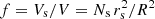 , measures the portion of a coronal region volume, V, filled with strands with a total volume Vs. The coronal region of volume V could have any shape but we have assumed a cylindrical volume with radius R for simplicity. This cylinder is physically meaningless in this work and it just delimits the region where the strands are placed. We also assume no boundary layer between the strand and the external corona (i.e. only a Heavyside function). This therefore eliminates the resonant absorption mechanism in our model.
In our study we consider different distributions with Ns = 1, 5, 10, 20, 30, 40, 50, 60, and 100 parallel strands. We use the T-matrix technique to find the normal modes of the system as explained in Sect. 3. Considering systems larger than 100 strands is difficult for numerical reasons. In Fig. 1 we have plotted the strand distribution for 20, 60, and 100 strands. In addition, the region within the square delimits an area of 6 × 6 Mm2 representative of a small portion of an AR corona. In principle the size of this region is arbitrary but we have selected this size in order to have a sufficiently large number of tubes inside. Henceforth, this area is our region of interest (ROI). From the figure, we see that only the 100 strands configuration covers the ROI. We will see that the vibrations in the square area are not fully described by the normal modes of the 100 strands system. However, with this limited system of 100 strands, we can understand the complexity of the oscillations of the strands in the ROI.
 |
Fig. 1. Sketch of the cross-section of a multi-stranded AR model, which consists of (a) Ns = 20, (b) Ns = 60, and (c) Ns = 100, homogeneous strands of densities ρs and radii rs. In the figure, the strands are represented by their external surface of radius rs (thick solid lines). The external medium to the strands consists of coronal material with density ρc. |
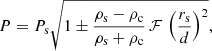
The strands have a length L = 100 Mm and radius rs = 0.2 Mm, which are typical values in agreement with observations (see Sect. 1). Each individual strand, labelled as j, is placed in the xy-plane in a position rj = xj ex + yj ey. These positions in the xy-plane are randomly generated inside the circular area of radius R. In order to keep a constant filling factor,  . These positions should fulfil the condition |rj| ≤ R − rs in order to have all the strands inside the circular area with radius R. In addition, the minimum distance between any two strands i and j is dij ≥ dmin = 𝒮 2 rs. With the arbitrary parameter 𝒮, we control the minimum distance between the strands. With 𝒮 = 1 the surfaces of the strands can be in contact. We have chosen 𝒮 = 1.692 in order to have a more or less uniform distribution of strands. In this situation, dmin = 0.68 Mm. We additionally consider a typical filling factor of f = 0.2 in agreement with the observed values (see Sect. 1). For the particular cases shown in Fig. 1, the strands cover a circular surface of radius R = 2.00, 3.46, and 4.47 Mm respectively. We assume a strand density ρs = 3.5 ρc in terms of the background coronal density, being ρc = 2 × 10⁻¹³ kg m−3, and a magnetic field intensity B = 5 Gauss. With these parameters, the individual kink period of each strand is Ps = 5 min. This period is a typical value for loop oscillations but also for the transverse waves of the solar corona (e.g. Tomczyk et al. 2007).
3. Collective normal modes: clustering
We first show how the normal modes are established in a large system of strands. We consider the example with Ns = 60 strands shown in Fig. 1b. The normal modes of the system depend on the number of strands and their spatial distribution (Luna et al. 2009, 2010). We have found the normal modes of the whole strand system using the T-matrix technique by Luna et al. (2009). In general, in the strand systems, the individual period Ps splits into a virtually infinite number of frequencies. The collective frequencies are distributed on both sides of the individual strand frequency (see Fig. 2). According to Luna et al. (2010) the normal modes can be classified according to their frequency: modes with frequencies below the central frequency, 2 π/Ps, are called Low modes (right-hand side of the Ps line in Fig. 2). Mid modes are those with periods similar to 2 π/Ps, and finally the solutions with frequencies above the central frequency are called High modes (on the left-hand side of the Ps line in Fig. 2). In the Low modes the fluid between the tubes follows the motion of the strands, resulting in a small perturbation of the magnetic pressure. In contrast, in the High modes, the fluid between tubes is compressed or rarefied with important perturbations of the pressure. Mid modes consist of more complex motions of the strands. The distinction between Low and High is straightforward because both have frequencies lower or higher than the individual kink mode frequency, respectively. However, there is no clear transition between Low and Mid modes or Mid and High modes. In terms of periods, the collective oscillations are between the maximum period, PL, associated to the Low mode with the minimum frequency, and the minimum period, PH, associated to the High mode with the largest frequency. We note that the notation High and Low refers to the frequency and PL and PH correspond to periods with the highest and lowest period values, respectively, so that the subscripts refer to the mode frequency from which the period is derived. The period band has a width ΔP = PL − PH. In the case of 60 strands shown in Fig. 2, the period band ranges from PH = 4.63 min to PL = 5.34 min, with a bandwidth ΔP = 0.71 min. In terms of frequencies, the modes range from 3.12 to 3.6 mHz, which is a frequency split of 0.48 mHz.
 |
Fig. 2. Frequency distribution of the collective normal modes associated with the Ns = 60 case. We clearly see a distribution of periods around Ps = 5 min. The circles mark the periods of the modes whose spatial structure is displayed in Fig. 3. |
 |
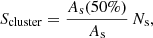
Fig. 3. Total pressure perturbation (colour field) and velocity field (arrows) of the fast collective normal modes. Panels a–d: first Low modes labelled from Mode 1 to 4. Central panels e–h: four examples of Mid modes. Panels i–l: last four High modes, Modes 409 to 412. |
In simple strand configurations with few closer elements, all the tubes participate in each collective mode. However, in more complex systems the situation is more involved. Figure 3 shows some of the normal modes of the system with 60 strands. The frequencies of the selected modes are marked with circles in the scatter period plot in Fig. 2. The top row (Figs. 3a–d) shows the first four Low modes and the bottom row (Figs. 3i–l) shows the last four High modes. From the figure, we can see that there are only subsets of tubes that participate in the collective oscillation. We have called this effect clustering and the subsets of tubes participating in each mode are the clusters. There is a correspondence between the Low and High modes. From Figs. 3a and l we see that both mode velocity fields are orthogonal. Similarly, the modes plotted in Figs. 3b and k are also orthogonal. In general, for each Low mode there is an orthogonal High mode. We can see this correspondence in all the modes plotted in Fig. 3. Thus a Low normal mode consists of a cluster of tubes oscillating in the direction that joins together the cluster elements. In contrast, the corresponding orthogonal High mode corresponds to motions perpendicular to that direction, compressing and rarefying the coronal plasma. Additionally, in the mode with the highest period, PL, the cluster of tubes that oscillates forms a chain of tubes moving and following one another. In the mode with the lowest period, PH, the same chain of tubes oscillates but in the perpendicular direction. Figures 3e–h show some Mid mode examples. These modes are also perpendicular between them like the pairs of Low and High modes. For example, the mode shown in Fig. 3e is perpendicular to the case shown in Fig. 3h and also to both modes shown in Figs. 3f and g. Mid modes have more spatial complexity and the structure is not clearly organised, forming large clusters. In these modes it seems that a large number of strands participate in the collective motions. However, small subsets are formed resembling a non-organised motion.
4. Dependence of the collective oscillations on the size of the system
In this section, we study the normal mode properties of systems with an increasing number of strands in order to understand the fundamental vibrations of the solar corona. In Sect. 3 we found that not all the strands participate in each normal mode and only a cluster of strands oscillate. Figure 4 shows the first and last normal modes with periods PL and PH, respectively, for Ns = 10, 20, 30, 50, and 100 cases. In all the cases the oscillations are in the form of clusters forming a chain of strands. In both modes, the oscillation is in the same chain of tubes. However, both Low and High modes are mutually perpendicular as discussed in Sect. 3. These chains can be closed (Figs. 4a and c) or open (Figs. 4e, g, and i). In all the situations, the normal modes associated to PL and PH are chains of the nearest set of strands with a separation between them close to dmin = 𝒮 2 rs = 0.68 Mm (see examples in Fig. 4). The rest of the Low and High modes also form clusters but due to space limitations they are not shown in Fig. 4. In order to estimate the number of tubes forming a cluster in each normal mode, we define the function
 (1)
(1)
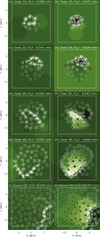 |
Fig. 4. First and last normal modes for Ns = 10, 20, 30, 30, and 100 cases in each row. Left column panels: first normal mode, associated with PH. Right column: last normal mode, associated with PL. |
where As(50%) is the cross-section area inside the tubes with a velocity equal to or larger than 50% of the maximum velocity of the normal mode and As is the cross-sectional area of all the tubes. Equation (1) is a good approximation of the number of tubes in a cluster. Figure 5 shows Scluster as function of the mode periods for Ns = 10, 20, 30, 60, and 100 cases. The shaded area covers the frequency range of the Mid modes for Ns = 60 and 100 cases (see Figs. 3e–h). The first and last modes, associated with PH and PL, form chains with less than 15 strands in all cases, in agreement Fig. 4. This may indicate that for Ns > 100, Scluster will be also small. We have computed the normal modes of a system of 200 strands confirming this tendency. However, for numerical reasons, we cannot find the Mid modes and the results show a large gap of modes in the central periods close to Ps. These chains are associated with the groups of closest tubes, d ≈ dmin, indicating that the size of the chains depends on the particular distribution of the tubes. In contrast, for the rest of Low and High modes the size of the clusters is much larger. From this figure, it is not clear if there is a general trend between the number of strands of the system and the size of the cluster. The magnitude Scluster/Ns seems to stabilise and it is more or less identical for 60 and 100 tubes. However, it is necessary to study much larger systems to find a general trend of Scluster/Ns.
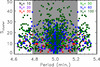 |
Fig. 5. Scatter plot of the approximate sizes of the cluster of strands of each normal mode given by the function Scluster as a function of the mode periods for Ns = 10, 20, 30, 60, and 100 cases in black, magenta, red, green, dark blue, and dark green, respectively. The shared area corresponds to the period range of the Mid modes for Ns = 100. |
In all the situations with Ns < 100, the system is inside the ROI of 6 × 6 Mm2 plotted as a white square area in Fig. 4 and hence the clusters are inside the area. However, for Ns = 100 in both clusters plotted in Figs. 4i and j the motion is partially outside the area. From Fig. 5 we see that many normal modes of this system have much larger clusters. Thus, many normal modes involve strands inside and outside the ROI. In a much larger system with Ns > 100, there will be even larger clusters partially inside and outside the area. The modes with clusters partially inside indicate the coupling of the vibrations of the ROI strands with the surrounding corona. In this sense, the range of the coupling of the strands of ROI extends beyond a system of 100 strands. Thus, the system of 100 strands is not fully representative of the oscillations in the ROI.
Figure 6 shows the normal mode periods for all the considered systems with Ns = 1, 5, 10, 20, 30, 40, 50, 60, and 100 strands. The period band, ΔP, increases rapidly between 1 and 10 strands, but for Ns ≥ 20, PL and PH reach an approximately constant value. With this plot, we obtain a relevant result: the period band or period splitting is independent of the size of the system for a sufficiently large Ns. In this sense, we obtain a general result that can be applied to an unlimited set of strands. The reason for this effect is that the two modes that flank the period band, that is, the modes with PH and PL, are chains of close tubes with a separation between them similar to dmin. In this sense, the period band depends on the random distribution of the strands and not on the size of the system.
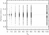 |
Fig. 6. Scatter plot of the normal mode periods of the systems considered a function of the number of strands, Ns = 1, 5, 10, 20, 30, 40, 50, 60, and 100. Each period is drawn as a small horizontal line except the case of Ns = 1 where an asterisk is used. The horizontal dotted line is the period of oscillation of an individual strand, Ps = 5 min. Both horizontal dashed lines are the analytic approximate expressions for PH and PL from Eq. (13). In all the situations the number of modes increases with the proximity to Ps and the plot looks like a continuous dark band. In the case of 100 strands, there is a gap associated with a numerical issue in the T-method. Near the central frequency, the T-matrix becomes singular and the method fails near the singularity. |
Additionally, the number of modes increases with Ns. For Ns = 5 there are a few scattered modes in the period band whereas for Ns = 100 they almost form a continuum of modes. The reason is that the number of clusters increases with the number of strands. For an infinite number of strands, the periods will tend to form a continuum between PH and PL. However, these modes are associated with clusters of strands in different spatial locations. Considering a finite volume, not all the normal modes have clusters inside the region and most of them are outside the finite volume. Therefore, the oscillations in a ROI will consist of a bunch of collective modes forming a very densely populated band of periods, but not a continuum.
For the ROI considered here and shown in Fig. 1, the normal modes of the Ns = 100 system are not a full description of the oscillations. Many collective normal modes are missing, with clusters involving tubes of the ROI and extending much beyond this region. However, due to the difficulty of numerically handling systems with a huge number of strands, we believe that the Ns = 100 case is a good qualitative representation of the vibrations of the ROI in terms of the obtained period band and complexity of the strand motions.
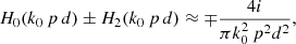
The normal mode with the highest period, PL, is formed by a chain of strands following one another (Fig. 3i). Additionally, in the normal mode with the lowest period, PH, the same chain of strands oscillates in the perpendicular direction (Fig. 3j). The periods of both modes define the period splitting associated with the strands’ interaction, Δ P = PL − PH, that is, without interaction Δ P = 0. In order to find an approximate expression for PL and PH we approximate the chain of strands as an infinite array of aligned tubes. In Fig. 7 the two modes with the highest period (top) and lowest period (bottom) are shown. From Luna et al. (2009) the total pressure perturbation, ψ, can be expressed as
![Mathematical equation: $$ \begin{aligned} \psi (\boldsymbol{r})=\sum _{{m}=-\infty }^{\infty } \alpha _{m}^{j} \left[J_{m} (k_{0} R_{j}) + T_{m m}^{j} H^{({1})}_{m} (k_{0} R_{j}) \right] e^{i {m} \varphi _{j}}, \end{aligned} $$](/articles/aa/full_html/2019/09/aa35850-19/aa35850-19-eq5.gif) (2)
(2)
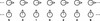 |
Fig. 7. Sketch of the normal modes associated with PL (top) and PH (bottom) of an infinite array of aligned strands along the horizontal axis. The strands are equally spaced with a separation d between the strands. Arrows indicate the direction of the motion. In the top panel, the strands move along the horizontal axis and in the bottom panel the strands move perpendicular to this axis. The three dots at both ends mean that the system continues to the infinity in both directions. The numbers indicate how the strands are labelled. |
for the external medium to the strands where
 (3)
(3)
 , Jm, and
  are the Bessel and Hankel functions of the first kind, and order m and
  are the T-matrix elements that represent the scattering properties of the jth tube (see Eq. (17) of Luna et al. 2009, for details). This field has two contributions associated with the excitation field to the j-tube and the scattered field by caused by the same tube. The excitation field on the j-tube is the combination of all the scattered field by the rest of the tubes. The coefficients
  are the expansion coefficients of order m that depend on the kz = π/L wave number and the angular frequency ω, and Rj and φj are the local polar coordinates centred at rj, defined through Rj = |r − rj| and cosφj = ex ⋅ (r − rj)/|r − rj|. As explained in Luna et al. (2009), it is possible to find an equation for the
  coefficients and mode frequencies ω. This equation is
 (4)
(4)
where φjq is the angle formed by the centre of the ith loop with respect to the centre of the jth flux tube. Equation (4) is formally an infinite system of equations for an infinite number of unknowns ( ). The condition that there is a non-trivial solution, that is that the determinant formed by the coefficients is set equal to zero, provides us with the dispersion relation (see details in Luna et al. 2009, 2010). For practical reasons the equation is approximated by truncating the system to a finite number of equations and unknowns by setting
  for azimuthal numbers greater than a truncation number (m > mt). To ensure the convergence of solutions, they must be independent of the truncation number mt. However, in this section in order to find an approximate dispersion relation, we assume that both modes of Fig. 7 are exclusively kink-like modes with the interaction of the strands through m = ±1.
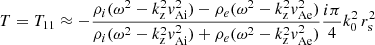
Both Eq. (4) for the central strand of Fig. 1 labelled 0 for m = ±1 are
![Mathematical equation: $$ \begin{aligned}&\frac{\alpha _{1}^{0}}{T} + \sum _{p=1}^{N}\left[ H_{0}(k_{0} \, p\, d)\left\{ \alpha _{1}^{2 p-1} +\alpha _{1}^{2 p} \right\} + H_{2}(k_{0} \, p\, d)\left\{ \alpha _{-1}^{2 p-1} +\alpha _{-1}^{2 p} \right\} \right]=0\end{aligned} $$](/articles/aa/full_html/2019/09/aa35850-19/aa35850-19-eq15.gif) (5)
(5)
![Mathematical equation: $$ \begin{aligned}&\frac{\alpha _{-1}^{0}}{T} + \sum _{p=1}^{N}\left[ H_{2}(k_{0} \, p\, d)\left\{ \alpha _{1}^{2 p-1} +\alpha _{1}^{2 p} \right\} + H_{0}(k_{0} \, p\, d)\left\{ \alpha _{-1}^{2 p-1} +\alpha _{-1}^{2 p} \right\} \right]=0 , \end{aligned} $$](/articles/aa/full_html/2019/09/aa35850-19/aa35850-19-eq16.gif) (6)
(6)
where T ≡ T−1−1 = T11,  and
and  . Additionally |rj − rs| = p d being p = 1, 2, 3, … and ei(n − m)φji = 1 in all the combinations of m and n. In these equations we see that strand 0 interacts with strands 1 and 2 that are at a distance d, with strands 3 and 4 at a distance 2d, and in general with a couple of strands at a distance p d. In principle N = ∞, but the interaction between strands is negligible at a distance larger than Nd. The reason is that the coupling between two strands is given by the functions H0(x) and H2(x), which are proportional to 1/x2 for a small x. In a general situation it is necessary to consider the equivalent equations to Eqs. (5) and (6) for all the strands solving the infinite equations system. However, we are interested in a situation where all the strands oscillate in the same way (see Fig. 7) where
 (7)
(7)
 (8)
(8)
and the system reduces to two unknowns, α and β, and two equations,
![Mathematical equation: $$ \begin{aligned}&\left[ \frac{1}{T} + \sum _{p=1}^{N}2 \, H_{0}(k_{0} \, p\, d) \right] \alpha + \sum _{p=1}^{N}2 \, H_{2}(k_{0} \, p\, d) \beta =0\nonumber \\&\sum _{p=1}^{N} 2 H_{2}(k_{0} \, p\, d) \alpha + \left[ \frac{1}{T} +\sum _{p=1}^{N}2 H_{0}(k_{0} \, p\, d)\right] \beta =0\nonumber \end{aligned} $$](/articles/aa/full_html/2019/09/aa35850-19/aa35850-19-eq21.gif)
for both α and β coefficients. We obtain the dispersion relation from the condition that there is a non-trivial solution of the system, namely
![Mathematical equation: $$ \begin{aligned} \left[ \frac{1}{T} + \sum _{p=1}^{N}2 \, H_{0}(k_{0} \, p\, d) \right]^2 - \left[ \sum _{p=1}^{N} 2 H_{2}(k_{0} \, p\, d) \right]^2 =0, \end{aligned} $$](/articles/aa/full_html/2019/09/aa35850-19/aa35850-19-eq22.gif) (9)
(9)
or
![Mathematical equation: $$ \begin{aligned} \frac{1}{T} + 2 \sum _{p=1}^{N} \left[ H_{0}(k_{0} \, p\, d) \pm H_{2}(k_{0} \, p\, d) \right] =0, \end{aligned} $$](/articles/aa/full_html/2019/09/aa35850-19/aa35850-19-eq23.gif) (10)
(10)
where the ± comes from the square root of the previous Eq. (9). The interaction of the strands is constrained by their neighbours. In this sense the term k0 p d is small and k0 rs ≪ 1. Under this approximation the combination of Hankel functions in Eq. (10) is
 (11)
(11)
and the T-matrix element can be approximated as
 (12)
(12)
(see Soler & Luna 2015, for details). Inserting these approximated expressions into Eq. (10) we obtain the period of both modes as
 (13)
(13)
where the + and − corresponds to PL and PH, respectively, and
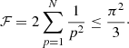 (14)
(14)
In this summation, N should be finite in order to keep k0 N d relatively small and the approximation (11) valid. In addition, the interaction is restricted to few neighbouring tubes. However, considering N → ∞, Eq. (14) converges to π2/3. Thus, the parameter is always ℱ < π2/3. We can consider that ℱ = π2/3 as a good approximation for large systems and that the period splitting ΔP is always constrained to lower values than those given by Eq. (13). With the values of the parameters described in Sects. 2 and 3 and assuming that d = dmin, we obtain PH = 4.58 and PL = 5.38 min. In Fig. 6, we have plotted these values as two horizontal dashed lines. We see that for a sufficiently large number of strands the maximum and minimum periods are well approximated by these analytic expressions. Expression (13) is very similar to Eq. (30) by Soler & Luna (2015) but with a correction factor, ℱ, associated to the multiple interaction.
Assuming that the period splitting is approximately symmetric, Ps ≈ 1/2(PL + PH) and with Eq. (13) we obtain
 (15)
(15)
With this expression we can see that the frequency splitting depends essentially on d, which is the minimum distance in the strand distribution, dmin. A shorter d involves a larger period splitting. It is important to note that d is not directly related to the filling factor, f. As explained in Sect. 2 in a random distribution of strands, the separation between strands ranges from a minimum to a maximum value. Then the group of strands with the minimum separation between them, dmin, determines the maximum period splitting, ΔP.
5. Non-identical tubes
The aim of this work is to understand the vibrations of a large region of the AR corona. The strands within this region have different tube lengths because of the three-dimensional topology of the field. In Luna et al. (2009) we found that differences in the strand Alfvén frequencies, that is, kz vA, reduce or avoid the coupling between the strand oscillations (see also Soler et al. 2009). Thus a difference in strand lengths may result in a decoupling of the AR strands. We can estimate the strand length differences by assuming semicircular shapes of the field lines in the region. The central tube has a length πL and the tubes of the periphery of the region πL(1 ± ϵ). Considering the ROI shown in Fig. 3 and with L = 100 Mm, ϵ = 0.04 (i.e. 4% of L). Properly accounting for the differences in tube lengths involves a fully three-dimensional study, but our approach is restricted to 2.5 dimensions assuming that all the field lines have identical lengths. However, we can mimic the effect of strand length differences by considering density differences. The relevant factor in strand coupling is the Alfvén frequency, kz vA. Thus a variation in length πL(1 ± ϵ) is equivalent to a density variation ρ (1 ± ϵ)2 in order to keep the variation in the Alfvén frequency the same,
 (16)
(16)
In addition, for a small ϵ, (1 ± ϵ)2 ≈ 1 ± 2 ϵ. Thus in our situation, a length variation of 4% is equivalent to a density variation of 8%. This density variation probably has a well-defined spatial distribution associated with the continuous variation of the field line lengths. However, the distribution of tube lengths in the xy-plane will depend on the AR field topology. We do not know this field length distribution a priori and we assume a random density distribution spanning an 8% variation around a fixed density.
Figure 8 shows the first and the last six modes of the case of 60 strands of Fig. 1 but with a strand density distribution ranging from 3.220ρc to 3.815ρc. We see that the modes are different when compared to those of the identical tubes shown in Fig. 3. For example, in the fundamental mode (Mode 1), the cluster of oscillating strands is different in both situations. The density variations in the strands affect the couplings between them and in general new clusters appear. The correspondence we found in Sect. 3 between Low and High modes is lost as we see in Figs. 8a and l. It is remarkable that in a situation with strand differences, the coupling remains. The periods PL and PH are similar to those of the identical tubes case. In this sense, the results of the analysis of Sect. 4 can also be applied here and the approximate expression given by Eq. (13) remains valid for non-identical strands with small tube length differences.
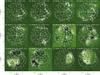 |
Fig. 8. Similar to Fig. 3 showing some normal modes of the identical strand distribution but with a random density distribution from 3.220ρc to 3.815ρc. The first six Low modes are plotted in panelsa–f whereas the last six High modes are in panelsg–l. |
6. Forward modelling
In this section, we generate synthetic images to compare with the observational evidence in a technique called forward-modelling. We consider the fundamental oscillations of the ROI and generate synthetic images with the FoMo code1 (Antolin & Van Doorsselaere 2013; Van Doorsselaere et al. 2016). We focus on the fingerprints of these vibrations in the synthetic Dopplergrams and the non-thermal line broadening. The vibrations of the strands system is a linear combination of the normal modes:
 (17)
(17)
where  is the nth normal mode velocity normalised to unity, ωn is the angular frequency of each normal mode, and An and ϕn are the amplitude and initial phase, respectively, of the velocity perturbation of the nth mode. In general, the amplitude and phase of each normal mode will depend on how the system is perturbed. We assume that the oscillatory spectrum is similar to the one observed by Tomczyk et al. (2007), which consists of a Gaussian function of width σ/2π = 1 mHz and centred at ω0/2π = 3.5 mHz shown in Fig. 9 as function of the period. The shaded area corresponds to the period range of the normal modes for a Ns = 100 system. The period spectrum of the normal modes is centred at 3.3 mHz (5 min), which is slightly shifted from the observed 3.5 mHz and covers a small portion of the measured spectral width. An additional consideration is that most of the collective mode periods are concentrated around 5 min as we see in Fig. 6. These are mostly Mid modes with a complex spatial structure. This introduces a bias in the distribution of the power given by Eq. (17) to the 5 min period. In order to compensate for this effect, we compute the frequency distribution of the normal modes, N(ωn), and then define the amplitude of each normal mode as
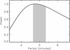 |
Fig. 9. Power spectra from Tomczyk et al. (2007) normalised to its maximum (see text for details). The shaded area corresponds to the period range of the normal modes of the case of 100 strands shown in Fig. 6. |
 (18)
(18)
where v0 is a scaling parameter. The velocities inside the tubes change with time and v0 is set to have a maximum velocity inside the tubes of 10 km s−1 during the temporal evolution. Thus, v0 will depend on the system of strands considered and the details of the linear combination. For the case of 100 strands considered in this section, v0 = 1.4 km s−1. We have defined the initial phase ϕn as a random number between 0 and 2π. The resulting complexity of the oscillations of the strands is not very sensitive to the selection of ϕn. The reason is that the periods are very different, producing important phase differences during the temporal evolution even for identical ϕn. Figure 10 shows the temporal evolution of a linear combination of collective normal modes by Eq. (17). We clearly see the complex motions of the strands in the accompanying animation. In each strand, the kink oscillation direction changes with time. This change in the direction of the kink oscillation leads to clockwise or anticlockwise motions changing with time in a complex fashion. Additionally, the amplitude of the motion also changes producing amplification or damping of the motions. These effects were already reported by Luna et al. (2010) with time-dependent numerical simulations. Stangalini et al. (2017) have recently found a similar motion in chromospheric elements that can be understood as strand footpoints. In this sense, the helical motions in chromospheric tubes can be the result of the collective oscillations of the coronal strands.
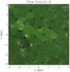 |
Fig. 10. First frame of the temporal evolution of the combination of normal modes of Eq. (17). Vectors are the velocity field and the green colour is the density perturbation. An animation of this figure is available online. |
In order to generate the synthetic images, we need all the thermodynamic magnitudes: density, gas pressure, and temperature. In our analytic calculations of the normal modes, we assume a zero-β plasma. In this approximation, we obtain the velocity, magnetic field, and density perturbations. The rest of the magnitudes are obtained with the linearised ideal MHD equations. We additionally assume that the equilibrium atmosphere is isothermal with T0 = 106 K and the equilibrium gas pressure is computed with the ideal gas law and the equilibrium density defined in Sect. 2. The gas pressure is not balanced at the strand surface between the internal and external medium. The reason is that we are in the zero-β approximation and hence the gas pressure gradients are negligible in the equilibrium configuration. An additional assumption here is that we neglect the Lagrangian displacement of the plasma. Thus each LOS always intersects the same strands. However, considering the Lagrangian displacements, the strands intersected by each LOS change with time, introducing additional complexity into the synthetic Dopplergrams. Although a more exact treatment for the forward modelling would need this to be taken into account, in this work we are only interested in the qualitative picture that is produced in Dopplergrams by fundamental vibrations.
For the forward modelling we chose the coronal spectral line of Fe IX 171.073 Å, forming at a temperature of 700 000 K approximately. We also considered hotter coronal lines such as Fe XII 193.509 Å but the results do not vary much since the perturbations on the temperature produced by the fundamental vibrations are very small. Therefore it is sufficient to only consider the results with the Fe IX line.
We consider an artificial slit placed perpendicularly to the strands’ direction and located at the loop apex. The artificial slit is placed along the x-axis in Fig. 1 and covers the ROI region. The LOS is along the y-direction in the figure. Due to the line tying of the magnetic field in the photosphere, the velocities of the strands are maximum at the apex of the tubes. Due to the finite size of our numerical box, any given LOS will cross more strands and less background corona for cases with a larger number of strands. Since the inter-strand space contributes differently to the emergent intensity than the space within strands, we have added dummy pixels at rest for each LOS ray to ensure that each ray has the same integrated length of background corona.
Figure 11 shows the time-distance diagrams on the artificial slit of the Doppler and line-broadening signals for Ns = 5, 30, and 100. The 5 strand case is the most simplistic situation (Fig. 11a). In this case, there are one or two strands for each LOS. We can identify the two left and the rightmost individual tubes. In these positions, the Dopplergrams show the intrinsic motions of the individual strands projected along the LOS. In the three tubes, we see a kink-like motion with a modulation of the amplitude. This modulation is associated with the interaction of the strands and it is a characteristic of the collective oscillation as we have discussed before (Fig. 10). This consists of a rotation of the direction of the oscillations in combination with damping or amplification of the motion. The maximum Doppler velocity is around 4 km s−1 but the actual strand velocities have a maximum of 10 km s−1. In these three cases the Doppler signal comes from individual tubes, which indicates that there is an intrinsic reduction of the observed velocity associated with the measurement (see Antolin & Van Doorsselaere 2013). This intrinsic reduction is less than a factor of three with respect to the actual velocity. The line broadening is in phase with the Doppler signal. An increase of the Doppler velocity involves an increase of the line broadening. This coincidence indicates that the Doppler signal is associated with the actual motions of the strands. The line broadening has an almost uniform value between 12 and 14 km s−1, which is larger than the actual velocity. This is due to the addition along the LOS of various velocity components, either from other strands and/or from the surrounding corona of each strand, which moves 90° out of phase to the strand. In x ∼ 0.3 Mm there are two strands in the same LOS (marked with a green arrow). In this region, there is a clear interference pattern associated with the integration of the Doppler signal along the LOS.
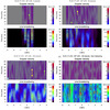 |
Fig. 11. Synthetic images for Ns = 100 strands from the FoMo code for (a) 5 strands, (b) 30 strands and (c) 100 strands cases. In (d) the case of 100 non-interacting strands is plotted (see text). Each panel shows time distances of the Doppler and line-broadening velocities. The arrows indicate some examples discussed in the text of regions with constructive (light blue), destructive (green), or amplified Doppler and line-broadening signals (yellow). |
For the case of 30 strands the situation is more complex (Fig. 11b). In the central region, there are several strands for each LOS. The Doppler pattern is very complex in the central region. The reason is that the integration of the Doppler signal along the LOS can produce constructive or destructive interference patterns. For example, in x = −1.6 Mm (marked with a green arrow) there is a minimum of the Doppler signal but a large line broadening. This indicates opposite motions of the plasma in this LOS that produce a cancellation of the Doppler signal and a line broadening. It is important to note that the fundamental vibrations considered here do not significantly perturb the temperature. Hence, the line broadening mostly corresponds to non-thermal line broadening and therefore gives an estimate of the variance of the Doppler velocity along the LOS. In contrast, at x = 0.4 Mm (light blue arrow) there is an enhancement of the Doppler signal with a moderate broadening signal suggesting a constructive interference along the LOS. Around x ∼ −0.7 Mm (yellow arrow) there are large Doppler velocity and line-broadening signals indicating that the Doppler signal is showing the motion of an individual strand.
Figure 11c shows the most complex situation with 100 strands. Both Doppler velocity and line-broadening time-distance diagrams show very complex patterns. The green and blue arrows show examples where the integration produces destructive or constructive interference, respectively. Due to the complexity of the patterns it is difficult to distinguish regions with significant Doppler signal and a large broadening associated with the collective oscillations of the strands. The two-headed yellow arrow shows the region where a collective oscillation starts and ends. However, in most cases, it is almost impossible to isolate the individual strand motions from their surroundings due to the complexity of the diagrams. As in the situation in the case marked with the yellow arrow, they appear surrounded by constructive and destructive patterns.
In order to distinguish the collective oscillations with respect to a non-interacting system, we have considered the same 100 strand distribution but with each strand oscillating individually with a kink mode. The initial phase of the oscillations and the direction of the motion have been randomly generated between 0 and 2π. The oscillation amplitude of each strand is fixed to 10 km s−1. The strand densities have been randomly generated in order to have a kink oscillation period between 4.637 and 5.338 min as the range of periods of the collective modes. Figure 11d shows the Doppler velocity and line-broadening time-distance diagrams. The Doppler velocity pattern also shows a complex structure of cancellation and superposition of the signals. It is thus difficult to distinguish it from the interacting strands case (Fig. 11c). In contrast, the line-broadening diagram is clearly different from the interacting strands case. The line broadening appears more uniform and individual strands seem more easily distinguishable. The reason is that the individual strands always oscillate with the same velocity amplitude. Regions with large broadening are produced when two strands oscillate in opposite directions. Conversely, regions with a reduction of the line broadening coincide with regions with an increase of the Doppler velocities due to constructive interference. In this situation, the complexity of the diagrams is associated with the interference pattern of the motions of the strands but not with the complexity of the motions of the strands.
Figure 12a shows the histogram of the Doppler velocities in both cases of 100 strands with interaction (“vibrations”) or without interaction (“random”). In the non-interacting tubes case, both the Doppler velocity and line-broadening distributions are broader. In the interacting tubes case, the motions of the strands are more complex, with rotations of the direction of the kink oscillations, damping, and amplifications producing narrower distributions. Similarly, the peak of the line-broadening distribution for the interacting tubes case has a smaller value, indicating less destructive interference. In Fig. 12c we have plotted the rms value of the Doppler velocities as a function of the line-broadening velocities. Both situations are clearly different. For the interacting strands, there is a clear positive correlation between both magnitudes for Doppler velocities smaller than 1.2 km s−1. This is due to the existence of regions of amplified Doppler velocity and line broadening associated with the individual motions of the strands that we have discussed previously. For the non-interacting case, any LOS will have, on average, the same variation of Doppler velocities, thereby leading to a roughly equal line width and no correlation. For Doppler velocities larger than 1.2 km s−1 the correlation is unclear and/or statistically not significant since the number of pixels in the histogram bins at these high velocity values is small. The correlation between the line broadening and the Doppler velocities is an important result that may allow us to distinguish between random individual oscillations and collective vibrations of the corona.
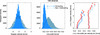 |
Fig. 12. (a) Doppler velocity. (b) Line width distributions for the 100 strand case with interactions (“interacting”) and without interactions (“non-interacting”). (c) rms value in line width for each bin of the velocity histogram against the rms value for the same pixels. Blue and red symbols in this panel correspond, respectively, to positive and negative Doppler velocities. |
7. Discussion and conclusions
In this work, we study the collective oscillations of the AR corona under the hypothesis that it is composed of a myriad of strands. We have found that in the collective modes, not all the strands participate in the motion. The modes are formed by clusters of tubes oscillating in different ways. Additionally, the modes with the lowest and the highest periods form a chain of strands. The periods distribute over a wide band of values. The width of the band increases with the number of strands but rapidly reaches an approximately constant value. Thus, for a sufficiently large number of strands the period range is independent of the size of the system. We have found an approximate expression for the minimum and maximum periods of the band. Our findings indicate that the frequency band associated with the fine structure of the corona depends on the strand configuration and the minimum distance between strands. The chains of strands associated to the highest and lowest periods are formed by the strands with the shortest distance between them. The size of this cluster is independent of the size of the system. However, for the rest of modes the cluster sizes increase with the size of the system. This indicates that the motion of one strand is influenced by the motions of distant strands. In this sense, in a finite volume of the corona, the oscillations of the strands inside the region are coupled to the strands outside of the region.
We have produced synthetic images of Doppler velocities and line broadening in order to find observational signatures of these fundamental vibrations. We consider the strands in a finite volume of the corona and the synthetic images are time-distance diagrams in a slit perpendicular to the axis of the strands. The strands of the region vibrate with a linear combination of collective normal modes. Both Doppler velocity and line width diagrams show a complex pattern. Part of this complexity is associated with the cancellation and superposition of the velocities along the LOS. However, the collective motions of the strands introduce additional complexity to the diagrams in terms of additional ordered motions (or less randomness in the system). We generated a situation without interaction (i.e. pure random motions) between strands and we found a clear difference. In the non-interacting strands situation, the line broadening is not correlated with the Doppler velocity. In contrast, in the interacting tubes case, the line broadening shows a positive correlation with Doppler velocities. We interpret this as a signature of the collective nature of the strand oscillations, however, it is a weak confirmation of the model because other models can also produce a positive correlation. Computational limitations restrict our models to systems with a maximum of 100 strands. Increasing the number of strands will result in collective effects affecting more strands. It will increase the non-uniformity of the collective signatures. In addition, the consideration of the background and foreground corona can reduce or amplify these collective signatures. Observational signatures from improved models will display more complex line broadening and Doppler velocity patterns. This work motivates future research in this direction by considering a much larger strands system. Although we have focused in this work on the assumption of a corona, which is composed of strands, the same results apply to a multitude of flux tubes distributed in a similar fashion. We have found that due to the nature of the solar corona as composed of elemental strands and/or flux tubes, it harbours a kind of collective of vibrations that we have called fundamental vibrations. These vibrations cannot exist in a uniform corona or without coupling between the motion of strands.
This work is a first step to further consider fast MHD wave propagation in the corona and the influence of the fine structure on it. The waves are resonantly scattered in the non-uniform corona. The frequencies of the waves that are scattered are the frequencies of the fundamental vibrations of the corona. The existence of the fine structure can affect the propagation of the energy and the coronal energy budget as has already been pointed out by de Moortel & Pascoe (2012) and Van Doorsselaere et al. (2014). The propagation of waves in a structured corona will be considered in a future study. Should results on the collective nature of periodic standing waves remain valid for propagating waves, this would reinforce the conclusion by McIntosh & De Pontieu (2012) that the origin of the positive correlation between Doppler velocities and line broadening is the kink wave nature of propagating waves.
Movies
Movie of Fig. 10 Access Supplementary Material
Acknowledgments
M. Luna acknowledges the support by the Spanish Ministry of Economy and Competitiveness (MINECO) through projects AYA2014-55078-P and under the 2015 Severo Ochoa Programme MINECO SEV-2015-0548. R.O. acknowledges support from the Spanish Ministry of Economy and Competitiveness (MINECO) and FEDER funds through project AYA2017-85465-P. P.A. acknowledges funding from his STFC Ernest Rutherford Fellowship (No. ST/R004285/1). M.L., R.O., and P.A. acknowledge support from the International Space Science Institute (ISSI), Bern, Switzerland to the International Team 401 “Observed Multi-Scale Variability of Coronal Loops as a Probe of Coronal Heating” (P.I. Clara Froment and Patrick Antolin). I.A. acknowledges financial support from the Spanish Ministerio de Ciencia, Innovación y Universidades through project PGC2018-102108-B-I00 and FEDER funds.
References
- Anfinogentov, S. A., Nakariakov, V. M., & Nisticò, G. 2015, A&A, 583, A136 [NASA ADS] [CrossRef] [EDP Sciences] [Google Scholar]
- Antolin, P., & Rouppe van der Voort, L. 2012, ApJ, 745, 152 [NASA ADS] [CrossRef] [Google Scholar]
- Antolin, P., & Van Doorsselaere, T. 2013, A&A, 555, A74 [NASA ADS] [CrossRef] [EDP Sciences] [Google Scholar]
- Antolin, P., Yokoyama, T., & Van Doorsselaere, T. 2014, ApJ, 787, L22 [NASA ADS] [CrossRef] [Google Scholar]
- Antolin, P., Okamoto, T. J., Pontieu, B. D., et al. 2015, ApJ, 809, 72 [NASA ADS] [CrossRef] [Google Scholar]
- Antolin, P., Moortel, I. D., Doorsselaere, T. V., & Yokoyama, T. 2017, ApJ, 836, 219 [NASA ADS] [CrossRef] [Google Scholar]
- Arregui, I., Terradas, J., Oliver, R., & Ballester, J. L. 2007, A&A, 466, 1145 [NASA ADS] [CrossRef] [EDP Sciences] [Google Scholar]
- Arregui, I., Terradas, J., Oliver, R., & Ballester, J. L. 2008, Waves and Oscillations in the Solar Atmosphere: Heating and Magneto-Seismology, 247, 133 [NASA ADS] [Google Scholar]
- Aschwanden, M. J., Fletcher, L., Schrijver, C. J., & Alexander, D. 1999, ApJ, 520, 880 [NASA ADS] [CrossRef] [Google Scholar]
- Brooks, D. H., Warren, H. P., & Ugarte-Urra, I. 2012, ApJ, 755, L33 [NASA ADS] [CrossRef] [Google Scholar]
- Brooks, D. H., Warren, H. P., Ugarte-Urra, I., & Winebarger, A. R. 2013, ApJ, 772, L19 [NASA ADS] [CrossRef] [Google Scholar]
- Brooks, D. H., Reep, J. W., & Warren, H. P. 2016, ApJ, 826, L18 [NASA ADS] [CrossRef] [Google Scholar]
- Cirtain, J. W., Golub, L., Winebarger, A. R., et al. 2013, Nature, 493, 501 [NASA ADS] [CrossRef] [Google Scholar]
- de Moortel, I., & Pascoe, D. J. 2012, ApJ, 746, 31 [NASA ADS] [CrossRef] [Google Scholar]
- de Pontieu, B., Title, A. M., Lemen, J. R., et al. 2014, Sol. Phys., 289, 2733 [NASA ADS] [CrossRef] [Google Scholar]
- Díaz, A. J., & Roberts, B. 2006, A&A, 458, 975 [NASA ADS] [CrossRef] [EDP Sciences] [Google Scholar]
- Díaz, A. J., Oliver, R., & Ballester, J. L. 2005, A&A, 440, 1167 [NASA ADS] [CrossRef] [EDP Sciences] [Google Scholar]
- Esmaeili, S., Nasiri, M., Dadashi, N., & Safari, H. 2016, J. Geophys. Res.: Space Phys., 121, 9340 [NASA ADS] [CrossRef] [Google Scholar]
- Jing, J., Xu, Y., Cao, W., et al. 2016, Sci. Rep., 6, 24319 [NASA ADS] [CrossRef] [Google Scholar]
- Klimchuk, J. A. 2015, Philos. Trans. R. Soc. A: Math. Phys. Eng. Sci., 373, 20140256 [NASA ADS] [CrossRef] [Google Scholar]
- Landi, E., Miralles, M. P., Curdt, W., & Hara, H. 2009, ApJ, 695, 221 [NASA ADS] [CrossRef] [Google Scholar]
- Lemen, J. R., Title, A. M., Akin, D. J., et al. 2011, Sol. Phys., 275, 17 [Google Scholar]
- Luna, M., Terradas, J., Oliver, R., & Ballester, J. L. 2006, A&A, 457, 1071 [NASA ADS] [CrossRef] [EDP Sciences] [Google Scholar]
- Luna, M., Terradas, J., Oliver, R., & Ballester, J. L. 2008, ApJ, 676, 717 [NASA ADS] [CrossRef] [Google Scholar]
- Luna, M., Terradas, J., Oliver, R., & Ballester, J. L. 2009, ApJ, 692, 1582 [NASA ADS] [CrossRef] [Google Scholar]
- Luna, M., Terradas, J., Oliver, R., & Ballester, J. L. 2010, ApJ, 716, 1371 [NASA ADS] [CrossRef] [Google Scholar]
- Magyar, N., & Van Doorsselaere, T. 2016, ApJ, 823, 82 [NASA ADS] [CrossRef] [Google Scholar]
- McIntosh, S. W., & De Pontieu, B. 2012, ApJ, 761, 138 [NASA ADS] [CrossRef] [Google Scholar]
- Morton, R. J., Weberg, M. J., & McLaughlin, J. A. 2019, Nat. Astron., 3, 223 [NASA ADS] [CrossRef] [Google Scholar]
- Nakariakov, V. M. 1999, Science, 285, 862 [NASA ADS] [CrossRef] [PubMed] [Google Scholar]
- Nakariakov, V. M., & Verwichte, E. 2005, Sol. Phys., 2, 3 [Google Scholar]
- Ofman, L. 2009, ApJ, 694, 502 [NASA ADS] [CrossRef] [Google Scholar]
- Peter, H., Bingert, S., Klimchuk, J. A., et al. 2013, A&A, 556, A104 [NASA ADS] [CrossRef] [EDP Sciences] [Google Scholar]
- Scharmer, G. B., Narayan, G., Hillberg, T., et al. 2008, ApJ, 689, L69 [NASA ADS] [CrossRef] [Google Scholar]
- Scullion, E., van der Voort, L. R., Wedemeyer, S., & Antolin, P. 2014, ApJ, 797, 36 [NASA ADS] [CrossRef] [Google Scholar]
- Soler, R., & Luna, M. 2015, A&A, 582, A120 [NASA ADS] [CrossRef] [EDP Sciences] [Google Scholar]
- Soler, R., Oliver, R., & Ballester, J. L. 2009, ApJ, 693, 1601 [NASA ADS] [CrossRef] [Google Scholar]
- Stangalini, M., Giannattasio, F., Erdelyi, R., et al. 2017, ApJ, 840, 19 [NASA ADS] [CrossRef] [Google Scholar]
- Tomczyk, S., & McIntosh, S. W. 2009, ApJ, 697, 1384 [NASA ADS] [CrossRef] [Google Scholar]
- Tomczyk, S., McIntosh, S. W., Keil, S. L., et al. 2007, Science, 317, 1192 [NASA ADS] [CrossRef] [PubMed] [Google Scholar]
- Tousey, R., Bartoe, J.-D. F., Bohlin, J. D., et al. 1973, Sol. Phys., 33, 265 [NASA ADS] [Google Scholar]
- Tsuneta, S., Ichimoto, K., Katsukawa, Y., et al. 2008, Sol. Phys., 249, 167 [NASA ADS] [CrossRef] [Google Scholar]
- Vaiana, G. S., Reidy, W. P., Zehnpfennig, T., VanSpeybroeck, L., & Giacconi, R. 1968, Science, 161, 564 [NASA ADS] [CrossRef] [Google Scholar]
- Vaiana, G. S., Davis, J. M., Giacconi, R., et al. 1973, ApJ, 185, L47 [NASA ADS] [CrossRef] [Google Scholar]
- Van Doorsselaere, T., Ruderman, M. S., & Robertson, D. 2008, A&A, 485, 849 [NASA ADS] [CrossRef] [EDP Sciences] [Google Scholar]
- Van Doorsselaere, T., Gijsen, S. E., Andries, J., & Verth, G. 2014, ApJ, 795, 18 [NASA ADS] [CrossRef] [Google Scholar]
- Van Doorsselaere, T., Antolin, P., Yuan, D., Reznikova, V., & Magyar, N. 2016, Front. Astron. Space Sci., 3, 72 [Google Scholar]
- Van Doorsselaere, T., Antolin, P., & Karampelas, K. 2018, A&A, 620, A65 [NASA ADS] [CrossRef] [EDP Sciences] [Google Scholar]
- van Speybroeck, L. P., Krieger, A. S., & Vaiana, G. S. 1970, Nature, 227, 818 [NASA ADS] [CrossRef] [Google Scholar]
- Warren, H. P., Ugarte-Urra, I., Doschek, G. A., Brooks, D. H., & Williams, D. R. 2008, ApJ, 686, L131 [NASA ADS] [CrossRef] [Google Scholar]
- Young, P. R., O’Dwyer, B., & Mason, H. E. 2011, ApJ, 744, 14 [Google Scholar]
- Zimovets, I. V., & Nakariakov, V. M. 2015, A&A, 577, A4 [NASA ADS] [CrossRef] [EDP Sciences] [Google Scholar]
All Figures
|
Fig. 1. Sketch of the cross-section of a multi-stranded AR model, which consists of (a) Ns = 20, (b) Ns = 60, and (c) Ns = 100, homogeneous strands of densities ρs and radii rs. In the figure, the strands are represented by their external surface of radius rs (thick solid lines). The external medium to the strands consists of coronal material with density ρc. |
| In the text | |
|
Fig. 2. Frequency distribution of the collective normal modes associated with the Ns = 60 case. We clearly see a distribution of periods around Ps = 5 min. The circles mark the periods of the modes whose spatial structure is displayed in Fig. 3. |
| In the text | |
|
Fig. 3. Total pressure perturbation (colour field) and velocity field (arrows) of the fast collective normal modes. Panels a–d: first Low modes labelled from Mode 1 to 4. Central panels e–h: four examples of Mid modes. Panels i–l: last four High modes, Modes 409 to 412. |
| In the text | |
|
Fig. 4. First and last normal modes for Ns = 10, 20, 30, 30, and 100 cases in each row. Left column panels: first normal mode, associated with PH. Right column: last normal mode, associated with PL. |
| In the text | |
|
Fig. 5. Scatter plot of the approximate sizes of the cluster of strands of each normal mode given by the function Scluster as a function of the mode periods for Ns = 10, 20, 30, 60, and 100 cases in black, magenta, red, green, dark blue, and dark green, respectively. The shared area corresponds to the period range of the Mid modes for Ns = 100. |
| In the text | |
|
Fig. 6. Scatter plot of the normal mode periods of the systems considered a function of the number of strands, Ns = 1, 5, 10, 20, 30, 40, 50, 60, and 100. Each period is drawn as a small horizontal line except the case of Ns = 1 where an asterisk is used. The horizontal dotted line is the period of oscillation of an individual strand, Ps = 5 min. Both horizontal dashed lines are the analytic approximate expressions for PH and PL from Eq. (13). In all the situations the number of modes increases with the proximity to Ps and the plot looks like a continuous dark band. In the case of 100 strands, there is a gap associated with a numerical issue in the T-method. Near the central frequency, the T-matrix becomes singular and the method fails near the singularity. |
| In the text | |
|
Fig. 7. Sketch of the normal modes associated with PL (top) and PH (bottom) of an infinite array of aligned strands along the horizontal axis. The strands are equally spaced with a separation d between the strands. Arrows indicate the direction of the motion. In the top panel, the strands move along the horizontal axis and in the bottom panel the strands move perpendicular to this axis. The three dots at both ends mean that the system continues to the infinity in both directions. The numbers indicate how the strands are labelled. |
| In the text | |
|
Fig. 8. Similar to Fig. 3 showing some normal modes of the identical strand distribution but with a random density distribution from 3.220ρc to 3.815ρc. The first six Low modes are plotted in panelsa–f whereas the last six High modes are in panelsg–l. |
| In the text | |
|
Fig. 9. Power spectra from Tomczyk et al. (2007) normalised to its maximum (see text for details). The shaded area corresponds to the period range of the normal modes of the case of 100 strands shown in Fig. 6. |
| In the text | |
|
Fig. 10. First frame of the temporal evolution of the combination of normal modes of Eq. (17). Vectors are the velocity field and the green colour is the density perturbation. An animation of this figure is available online. |
| In the text | |
|
Fig. 11. Synthetic images for Ns = 100 strands from the FoMo code for (a) 5 strands, (b) 30 strands and (c) 100 strands cases. In (d) the case of 100 non-interacting strands is plotted (see text). Each panel shows time distances of the Doppler and line-broadening velocities. The arrows indicate some examples discussed in the text of regions with constructive (light blue), destructive (green), or amplified Doppler and line-broadening signals (yellow). |
| In the text | |
|
Fig. 12. (a) Doppler velocity. (b) Line width distributions for the 100 strand case with interactions (“interacting”) and without interactions (“non-interacting”). (c) rms value in line width for each bin of the velocity histogram against the rms value for the same pixels. Blue and red symbols in this panel correspond, respectively, to positive and negative Doppler velocities. |
| In the text | |
Current usage metrics show cumulative count of Article Views (full-text article views including HTML views, PDF and ePub downloads, according to the available data) and Abstracts Views on Vision4Press platform.
Data correspond to usage on the plateform after 2015. The current usage metrics is available 48-96 hours after online publication and is updated daily on week days.
Initial download of the metrics may take a while.