| Issue |
A&A
Volume 629, September 2019
|
|
|---|---|---|
| Article Number | A31 | |
| Number of page(s) | 20 | |
| Section | Extragalactic astronomy | |
| DOI | https://doi.org/10.1051/0004-6361/201935452 | |
| Published online | 30 August 2019 | |
Iron abundance distribution in the hot gas of merging galaxy clusters
1
SRON Netherlands Institute for Space Research, Sorbonnelaan 2, 3584 CA Utrecht, The Netherlands
e-mail: This email address is being protected from spambots. You need JavaScript enabled to view it.
2
Leiden Observatory, Leiden University, PO Box 9513, 2300 RA Leiden, The Netherlands
3
MTA-Eötvös University Lendület Hot Universe Research Group, Pázmány Péter sétány 1/A, Budapest, 1117, Hungary
4
Institute of Physics, Eötvös University, Pázmány Péter sétány 1/A, Budapest 1117, Hungary
5
Kavli Institute for the Physics and Mathematics of the Universe (WPI), University of Tokyo, Kashiwa 277-8583, Japan
6
Department of Physics, Bogazici University, 34342 Istanbul, Turkey
Received:
12
March
2019
Accepted:
6
June
2019
Abstract
We present XMM-Newton/EPIC observations of six merging galaxy clusters and study the distributions of their temperature, iron (Fe) abundance and pseudo-entropy along the merging axis. For the first time, we focused simultaneously, and in a comprehensive way, on the chemical and thermodynamic properties of the newly collided intra cluster medium (ICM). The Fe distribution of these clusters along the merging axis is found to be in good agreement with the azimuthally-averaged Fe abundance profile in typical non-cool-core clusters out to r500. In addition to showing a moderate central abundance peak, though less pronounced than in relaxed systems, the Fe abundance flattens at large radii towards ∼0.2−0.3 Z⊙. Although this shallow metal distribution is in line with the idea that disturbed, non-cool-core clusters originate from the merging of relaxed, cool-core clusters, we find that in some cases, remnants of metal-rich and low entropy cool cores can persist after major mergers. While we obtain a mild anti-correlation between the Fe abundance and the pseudo-entropy in the (lower entropy, K = 200−500 keV cm2) inner regions, no clear correlation is found at (higher entropy, K = 500−2300 keV cm2) outer radii. The apparent spatial abundance uniformity that we find at large radii is difficult to explain through an efficient mixing of freshly injected metals, particularly in systems for which the time since the merger is short. Instead, our results provide important additional evidence in favour of the early enrichment scenario in which the bulk of the metals are released outside galaxies at z > 2−3, and extend it from cool-core and (moderate) non-cool-core clusters to a few of the most disturbed merging clusters as well. These results constitute a first step toward a deeper understanding of the chemical history of merging clusters.
Key words: X-rays: galaxies: clusters / galaxies: clusters: intracluster medium / galaxies: abundances / shock waves
© ESO 2019
1. Introduction
In order to become the largest gravitationally bound structures seen in the Universe today, galaxy clusters grow in a hierarchical way, via not only accretion but also merging of surrounding (sub) haloes. The latter case is particularly interesting as major cluster mergers are the most energetic events since the Big Bang. During the merging process, the hot intra-cluster medium (ICM) in galaxy clusters is violently compressed and heated, and large amounts of thermal and non-thermal energy are released, giving rise to shock fronts and turbulence (Markevitch & Vikhlinin 2007). Shocks can propagate into the ICM (re)accelerating electrons (Bell 1987; Blandford & Eichler 1987), which may produce elongated and polarised radio structures known as radio relics via synchrotron radio emission (for a review, see Ferrari et al. 2008; Brunetti & Jones 2014). On the other hand, particle (re)acceleration by means of the turbulence in the ICM could generate unpolarised cluster-wide sources known as radio haloes (for a review, see Brunetti et al. 2001; Feretti et al. 2012; van Weeren et al. 2019).
The ICM is also known to be rich in metals, which originate mainly from core-collapse supernovae (SNcc) and type Ia supernovae (SNIa), which have been continuously releasing their nucleosynthesis products since the epoch of major star formation, about ten billion years ago (z ∼ 2−3) (Hopkins & Beacom 2006; Madau & Dickinson 2014). SNcc contribute primarily to the synthesis of light metals (O, Ne, Mg, Si and S). On the other hand, heavier metals (such as Ar, Ca, Mn, Fe, and Ni), together with the smaller relative contribution of Si and S, are produced by SNIa. Finally, C and N are mostly released by low-mass stars on the asymptotic giant branch (AGB). Once the metals are ejected to the ICM by SN or AGB stars, they are later transported, mixed, and redistributed via other processes, such as galactic winds (Kapferer et al. 2006, 2007; Baumgartner & Breitschwerdt 2009); ram-pressure stripping (Schindler et al. 2005; Kapferer et al. 2007); active galactic nucleus (AGN) outflows (Simionescu et al. 2008, 2009; Kapferer et al. 2009); or gas sloshing (Simionescu et al. 2010; Ghizzardi et al. 2014); among other processes. Detailed reviews on the observation of metals in the ICM include, for example Werner et al. (2008), Böhringer & Werner (2010), de Plaa (2013) and Mernier et al. (2018a).
In the last years, the Fe abundance distribution in galaxy clusters has been extensively studied using the different X-ray observatories (De Grandi & Molendi 2001; De Grandi et al. 2004; Baldi et al. 2007; Leccardi & Molendi 2008; Maughan et al. 2008; Matsushita 2011; Mernier et al. 2016, 2017; Mantz et al. 2017; Simionescu et al. 2017, 2019). The Fe radial distribution is different for cool-core (CC, i.e., dynamically relaxed) clusters and non-cool-core (NCC, i.e., dynamically disturbed) clusters. In the case of CC clusters, the Fe distribution shows a peak in the core, which decreases by up to ∼0.3r500 and flattens for larger radii. NCC clusters, however, have a flat distribution in the core and follow the same universal distribution as CC for outer radii. These abundance distributions do not present evidence of evolution from now until z ∼ 1 (McDonald et al. 2016; Mantz et al. 2017; Ettori et al. 2017). Moreover, recent X-ray observations with Suzaku (Fujita et al. 2008; Werner et al. 2013; Urban et al. 2017; Ezer et al. 2017; Simionescu et al. 2017) reveal a uniform radial distribution of around ∼0.2−0.3 Z⊙ in the outskirts of the galaxy clusters, which suggests an early enrichment of the ICM (i.e. z ∼ 2−3). Numerical simulations later showed that active galactic nuclei (AGN) feedback at early times is needed to explain these observations (e.g. Biffi et al. 2017, 2018a,b).
Whereas metals in the ICM have been extensively and systematically studied in CC and, to some extent, NCC clusters, the ICM enrichment in the extreme case of merging clusters has been poorly explored so far (except in a few specific cases; e.g. A3376, Bagchi et al. 2006; A3667, Lovisari et al. 2009; Laganá et al. 2019). Knowing in detail how metals are distributed across merging clusters, however, is a key ingredient in our understanding of the chemical evolution of large scale structures. On one hand metals act as passive tracers and may reveal valuable information on the dynamical history of the recently merged ICM. On the other hand, merging shocks could in principle trigger star formation in neighbouring galaxies (Stroe et al. 2015; Sobral et al. 2015), hence potentially contributing to the ICM enrichment to some extent (Elkholy et al. 2015). Metallicities in the shocked gas of such disturbed clusters, and their connection with their thermodynamical properties and star formation of their galaxies remain widely unexplored.
In this work, we present for the first time a study specifically devoted to the chemical state of merging clusters. For this purpose, we derive the spatial distribution of temperature, abundance (Fe), and pseudo-entropy from specifically selected regions of six merging galaxy clusters: CIZA J2242.8+5301, 1RXS J0603.3+4214, Abell 3376, Abell 3667, Abell 665, and Abell 2256. The principal characteristics of these clusters are summarised in Table 2. The first four clusters of the list are essentially major mergers hosting a double radio relic, while Abell 665 hosts a giant radio halo and Abell 2256 a prominent single radio relic together with a radio halo. The selection criteria of these clusters have been: (i) XMM-Newton observation availability, (ii) net exposure time > 25 ks (iii) bright and disturbed central ICM and (iv) probing a variety of diffuse radio features: we include merging clusters with double radio relics, a single radio relic and strong radio halo. This is not intended as a complete sample but rather as an exploratory first step towards future studies on metals in the ICM of merging clusters from larger observational samples. For this study, we report our results with respect to the protosolar abundances (Z⊙) reported by Lodders et al. (2009). We assume the cosmological parameters H0 = 70 km s−1 Mpc−1, ΩM = 0.27 and ΩΛ = 0.73. All errors are given at 1σ (68%) confidence level unless otherwise stated and the spectral analysis uses the modified Cash statistics (Cash 1979; Kaastra 2017).
2. Observations and data reduction
Table 1 summarises the XMM-Newton observations, the different pointings and the net exposure time used for the cluster survey analysis. All the data are reduced with the XMM-Newton Science Analysis System (SAS) v17.0.0, with the calibration files dated by June 2018. We used the observations from the MOS and pn detectors of the EPIC instrument and reduced them first with the standard pipeline commands emproc and epproc. Next, we filter the soft-proton (SP) flares by building Good Time Interval (GTI) files following the method detailed in Appendix A.1 of Mernier et al. (2015). This method consists of extracting light curves at the high energy range of spectrum (10−12 keV for MOS and 12−14 keV for pn) in bins of 100s. Then, the mean count rate, μ, and the standard deviation, σ, are calculated in order to apply a threshold of μ ± 2σ to the generated distribution. Therefore, all the time bins with a number of counts outside the interval μ ± 2σ are rejected. Afterwards, we apply the same process at the low energy range 0.3−2 keV with bins of 100s (Lumb et al. 2002). Only events satisfying the 2σ threshold in the two energy ranges mentioned above are further considered. The point source identification in the complete field of view (FOV) is done with the SAS task edetect_chain applied in four different bands (0.3−2.0 keV, 2.0−4.5 keV, 4.5−7.5 keV, and 7.5−12 keV). After this, we combine the detections in these four bands and exclude the point sources with a circular region of 10″ radius, except some larger sources where an appropriate radius has been applied. The 10″ radius size, as explained in Appendix A.2 of Mernier et al. (2015), is optimised for avoiding the polluting flux of the point sources and not reducing considerably the emission of the ICM. We keep the single, double, triple and quadruple events in MOS (pattern≤12) and only the single pixel events in pn (pattern==0). We also correct the out-of-time events from the pn detector1.
Observations and exposure times.
Cluster sample description.
3. Spectral analysis
3.1. Spectral analysis approach
In our spectral analysis of the clusters, we assume that the observed spectra include the following components (see EPIC MOS2 spectrum in Fig. 1): an optically thin thermal plasma emission from the ICM in collisional ionization equilibrium (CIE), the local hot bubble (LHB), the Milky Way halo (MWH), the cosmic X-ray background (CXB) and the non X-ray background (NXB), consisting of hard particle (HP) background and residual soft-proton (SP) component (see Sect. 3.2). An additional hot foreground (HF) component is included for CIZA J2242.8+5301 as suggested by Ogrean et al. (2013b) and Akamatsu et al. (2015). Further details about these components (and how we include them in the fits) are given in Sect. 3.2. The emission models are corrected for the cosmological redshift and absorbed by the galactic interstellar medium. The hydrogen column density value adopted for all the clusters is the weighted neutral hydrogen column density, NHI, estimated using the method of Willingale et al. (2013) 2. Previous work (e.g. Mernier et al. 2016; de Plaa 2017) noted that the total NH value (neutral + molecular hydrogen) may sometimes provide inaccurate fits whereas the weighted neutral hydrogen NHI values are generally closer to the best-fit NH values. Specifically, we have checked that leaving free the NH in our fits provides values that do not deviate more than ∼10% from the above estimates. The only exception is CIZA J2242.8+530, for which we need to leave the value of NH free within the range 0.8 × NH ≤ NHI ≤ 1.2 × NH, tot, where NH, tot is the weighted total (neutral and molecular) hydrogen column density (Willingale et al. 2013).
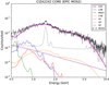 |
Fig. 1. EPIC MOS2 spectrum of CIZA2242 core (r = 1.5′). The solid black line represents the best-fit model. The cluster emission ICM and all background components (LHB, MHW, CXB, HF, HP and SP) are also shown. |
In our spectral analysis, we use SPEX3 (Kaastra et al. 1996, 2017) version 3.04.00 with SPEXACT (SPEX Atomic Code and Tables) version 3.04.00. We carry out the spectral fitting in different regions as detailed in the sections below. The redistribution matrix file (RMF) and the ancillary response file (ARF) are processed using the SAS tasks rmfgen and arfgen, respectively. The spectra of the MOS (energy range from 0.5 to 10 keV) and pn (0.6−10 keV) detectors are fitted simultaneously and binned using the method of optimal binning described in Kaastra & Bleeker (2016). We assume a single temperature structure in the collisional ionization equilibrium (cie model from SPEX) component for all the clusters (this assumption is justified in Sect. 3.3). Because the high temperature of merging clusters does not allow to measure other metals with reasonable accuracy, their abundances are coupled to Fe. The free parameters considered in this study are the temperature kT, the metal abundance Z and the normalisation Norm. In the case of CIZA J2242.8+5301, the column density NH is also free to vary.
3.2. Estimation of background spectra
A proper estimation of the background components is important especially in the regions where the emission of the cluster is low. This is particularly relevant outside of the core, where the spectrum can be background dominated. In this work, we model the background components directly from our spectra (Sect. 3.1) using the following list of components:
-
The LHB, modelled by a non-absorbed cie component with proto-solar abundance. The temperature is fixed to 0.08 keV.
-
The MWH, modelled by an absorbed cie component with proto-solar abundance. The temperature is free to vary except for CIZA J2242.8+5301 and Abell 3376, where it is fixed to 0.27 keV, following the values of Akamatsu et al. (2015) and Urdampilleta et al. (2018), respectively.
-
The CXB, modelled by an absorbed power law with a fixed Γ = 1.41 (De Luca & Molendi 2004). The normalisation is a fixed value for each cluster assuming the CXB flux of 8.07 × 10⁻¹⁵ W m−2 deg−2, taking into account a detection limit of Sc = 3.83 × 10⁻¹⁵ W m−2 and calculated with the CXBTools (de Plaa 2017). See details in Appendix B.2 of Mernier et al. (2015) 4.
-
The HF, modelled by an absorbed cie component with proto-solar abundance. The temperature is fixed to 0.7 keV.
-
The HP background, modelled by a broken power law (unfolded by the effective area) together with several instrumental Gaussian profiles (eight and nine for MOS and pn, respectively). The photon indices of the power laws and the centroid energies of the profiles have been taken from Tables B.1 and B.2 of Mernier et al. (2015), see their Appendix B.1 for more details. The normalisations are left free to vary.
-
The SP background, modelled by a power law (unfolded by the effective area). The power law index of the SP component is left free to vary between 0.1 and 1.4.
The estimation of the sky background components (LHB, MHW, and HF) is obtained from the offset regions (see green sectors in Figs. 2, 4, 8, 10, and 12) where a negligible (yet still modelled) thermal emission of the cluster is expected and the background is dominant. For Abell 3376 the values of Urdampilleta et al. (2018) are adopted. The parameters of the SP components are obtained fitting the total FOV (r = 15′) EPIC spectra, where the cie (i.e. ICM) parameters are also left free. Finally, the normalisation of every background component (except the HP background) has been fixed, rescaled on the sky area of each region and corrected for vignetting if necessary. The best-fit parameters for each cluster are listed in Appendix B.
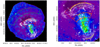 |
Fig. 2. Left panel: XMM-Newton smoothed image in the 0.3−10 keV band of CIZA2242. The red sectors represent the regions used for the radial temperature and abundance profiles. The green sector is the offset region used for the sky background estimation. Cyan circles are the point sources removed (with enlarged radius for clarity purpose). White contours are LOFAR radio contours. Right panel: enlarged image of CIZA2242. The BCGN and BCGS are marked with blue and black crosses, respectively. The solid yellow lines show the X-ray shocks position. |
3.3. Systematic uncertainties
We account for the effect of systematic uncertainties related to the ±10% variation in the normalisation of the sky background and non X-ray background components (Mernier et al. 2017). The contribution of these systematic uncertainties are further included in our analysis and results.
Mernier et al. (2017) and the posterior review of Mernier et al. (2018a) list other potential systematic uncertainties, which could affect the abundance measurements of this work. These include MOS-pn discrepancies due to residual EPIC cross-calibration, projection effects, atomic code and thermal structure uncertainties. The former has limited impact on the relative Fe abundance distribution as explained by Mernier et al. (2017). Although recent work of Liu et al. (2018) suggests that projection effects may have non-negligible observational biases on the observed abundance evolution in the core of CC clusters, the lack of strong emission gradients in merging clusters makes us confident that such a bias is limited in our case. Moreover, deprojecting merging cluster emission is very challenging, as by definition these systems are far from being spherically symmetric.
Uncertainties regarding the atomic codes are limited by the fact that we are using the update of the code SPEXACT and SPEX, which incorporate more precise modelling of the atomic processes and extensive compilation of transitions. However, uncertainties due to a not complete atomic database are still present (Hitomi Collaboration 2018) and their effects can be non-negligible (Mernier et al. 2018b).
For the thermal structure, we assume a single-temperature (1T) model. This is a simplified approximation; other more complex models reproducing Gaussian (gdem, de Plaa et al. 2006) or power-law (wdem, Kaastra et al. 2004) temperature distributions could represent better the inhomogeneities of the ICM. To quantify these possible effects, we have fitted the spectra assuming a simplified version of the gdem model using a 3T model with one main temperature free and the other two coupled with a factor of 0.64 and 1.56, respectively. We have realised the fits in the SPEXACT version 2.07.00 in order to significantly reduce the computing time. This version includes simpler atomic code and tables, which allows to fit the spectra faster, but with a similar accuracy as the most updated version (for more details, see Mernier et al. 2018b). We verify that the best-fit temperature of the main component in our 3T model remains within ±5% of the best-fit temperature obtained when assuming a 1T model. The relative emission measure of the other two components are less than 1% of the best-fit emission measure of the 1T model, and the variation in the abundance is less than 10%. This 1T-like behavior is not surprising as, unlike CC clusters, merging clusters do not exhibit a strong temperature gradient, and at these high temperatures the Fe abundance is almost entirely determined from the Fe-K line (which is unaffected by theFe-bias or the inverse Fe-bias, e.g. Buote 2000; Simionescu et al. 2009). For this reason and for simplicity we decide to maintain the 1T model and we will add these uncertainties to the other background systematic uncertainties as the thermal structure contribution.
4. Spectral analysis: individual clusters
4.1. CIZA J2242.8+5301
CIZA J2242.8+5301 (hereafter CIZA2242, also known as the “Sausage” cluster) is a massive (∼1015M⊙) and two-body (Jee et al. 2015) merging galaxy cluster at a redshift of z = 0.192. It was discovered in the second CIZA sample from the ROSAT All-Sky Survey and identified as a major-merger by Kocevski et al. (2007). van Weeren et al. (2010) studied CIZA2242 for the first time using WSRT, GMRT, and VLA. They observed a double radio relic feature located at ∼1.5 Mpc from the cluster centre. XMM-Newton and Chandra observations (Ogrean et al. 2013b, 2014) reveal a strongly disturbed and complex merger. In fact, the ICM presents an elongated X-ray morphology with a bullet shape bright edge in the south (S) and more irregular edge in the north (N), suggesting that the infalling direction is N to S. Akamatsu et al. (2015) estimate the time after the core passage to be ∼0.6 Gyr, in good agreement with the Sunyaev–Zel’dovich (SZ) analysis of Rumsey et al. (2017).
Finally, Stroe et al. (2014a, 2017), Stroe & Sobral (2015), Sobral et al. (2015) confirm an overdensity of Hα emitters, mainly cluster star-forming galaxies and AGNs, concentrated close to the subcores and northern post-shock region. The star-forming galaxies are found to be highly metal rich and to have strong outflows. The above mentioned authors propose that such an enhancement of the star formation ratio could be a shock-induced effect.
We fit the cluster emission and the background spectra (see Table B.1) in the sectors shown in Fig. 4, having excluded the point sources. We leave NH free to vary between 0.8 × NHI ≤ NH ≤ 1.2 × NH, Total, where NHI = 3.22 × 1021 cm−2 and NH, Total = 4.64 × 1021 cm−2 (Willingale et al. 2013), as explained in Sect. 3.1. The two circular regions are centred close to the two brightest cluster galaxies (BCGs) or subcores of the bimodal merger system described by Dawson et al. (2015) (BCGN:  ,
,  ; BCGS:
  ,
,  ). We use as centroid the southern “core”, because it contains the X-ray peak emission and is close to the southern BCG.
The best-fit parameters are shown in Table C.1, while the temperature and abundance distributions along the merging axis are plotted in Fig. 3. By convention, and for all the further relevant figures in this paper, the regions lying behind the projected main BCG trajectory are plotted with positive values on the x-axis. The temperature distribution presents a variation in the range between ∼8−10 keV within the inner regions of the X-ray emission. This temperature is higher in the last annular region, coincident with the post-shock region as described in Ogrean et al. (2014) and Akamatsu et al. (2015). These results are in good agreement within the uncertainties with the temperature map obtained by Ogrean et al. (2013b) and the radial profile of Akamatsu et al. (2015).
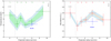 |
Fig. 3. Left panel: temperature distribution along the merging axis of CIZA2242. Right panel: abundance distribution along the merging axis of CIZA2242. The shaded areas represent the systematic uncertainties: green and orange shadows correspond to the background normalisation variation, and the blue one to the temperature structure. The shaded grey area shows the radio relic position. The dashed line shows the outer edge of the core spectral extraction region. The numbers and the BCGN blue point correspond to the regions and the red circle centred on BCGN, respectively, shown in Fig. 2. |
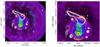 |
Fig. 4. Left panel: XMM-Newton smoothed image in the 0.3−10 keV band of 1RXSJ0603. The red sectors represent the regions used for the temperature and abundance distributions. The green sector is the offset region used for the sky background estimation. Cyan circles are the point sources removed, with enlarged radius for clarity purpose. White contours are LOFAR HBA radio contours. Right panel: enlarged image of 1RXSJ0603. The COREN and CORES are marked with blue and black crosses, respectively. The solid yellow and orange lines show the X-ray shock and cold front position. The numbers label the regions used in the spectral fitting. |
Between the two BCGs (sectors two to four) the Fe abundance is measured at its lowest value, between ∼0.2 and 0.3 Z⊙. Moreover, the abundance profile shows an apparent enhancement with a maximum value of ∼0.4 Z⊙ in sectors one and five, where the two BGCs are located. The northern BCG region evinces a lower abundance than the entire sector five. If we divide sector five in three regions, we obtain a gradient in the abundance and slight increase in the temperature towards the east, see Table C.1. BCGN coincides mostly with region 5b and the enhancement in abundance in sector five is mainly driven by region 5a.
4.2. 1RXS J0603.3+4214
1RXS J0603.3+4214 (hereafter 1RXSJ0603), also known as the “Toothbrush” cluster, is a bright, rich and massive cluster discovered by van Weeren et al. (2012) and located at z = 0.225. It hosts three radio relics and a giant (∼2 Mpc) radio halo elongated along the main merger axis S–N, which follows the X-ray emission morphology excluding the southernmost part (Ogrean et al. 2013a; Rajpurohit et al. 2018). Stroe et al. (2014b) found no enhancement of Hα emitters near the northern radio relic, with a star formation rate (SFR) consistent with that of blank field galaxies at z = 0.2. They concluded that the lack of Hα emitters could be possible because 1RXSJ0603 is a well evolved system, approximately ∼2 Gyr after the core passage.
As shown in Fig. 4, we use various sectors to fit the cluster emission and the background spectra (see Table B.2), excluding the point sources and using NHI = 2.15 × 1021 cm−2 (Willingale et al. 2013). We follow the X-ray emission S–N shape, coincident with the radio halo elongation with boxes four to eight, as well as the pre-shock region nine. We dedicate two circular sectors to the subcores of the main two subclusters, locating the brightest one in X-rays at the south (CORES:  ,
,  ) and the second at the north (COREN:
  ,
,  ). We use CORES as centroid for our temperature and abundance distributions along the merging axis (see Fig. 5).
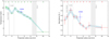 |
Fig. 5. Left panel: temperature distribution along the merging axis of 1RXSJ0603. Right panel: abundance distribution along the merging axis of 1RXSJ0603. The shaded areas represent the systematic uncertainties: the green shadow correspond to the background normalisation variation, and the blue one to the temperature structure. The shaded grey areas show the cold front and radio relic position. The dashed line shows the outer edge of the core spectral extraction region. The numbers and COREN blue point correspond to the regions and the red circle centred on COREN, respectively shown in Fig. 4. |
The best-fit parameters are presented in Table C.2 and are in good agreement with the previous X-ray studies by Ogrean et al. (2013a), Itahana et al. (2015), and van Weeren et al. (2016). The subcore temperatures (kT = 8.43 ± 0.27 keV for CORES and kT = 8.85 ± 0.36 keV for COREN) are consistent with van Weeren et al. (2016). Interestingly, we find a peak in Fe abundance located in the inner core, just behind the cold front (CF) (see Fig. 5; its location is approximated based on van Weeren et al. 2016). In the south, we see a slight temperature gradient towards the southern shock front, anticorrelated with a decrease in Fe abundance. The COREN shows the same abundance as the adjacent inner region, but a higher value than in the outer sectors (six to nine). It is possible that the gas belonging to this subcluster has been stripped during the merger and is mixing in that region. In the north, a gradual smooth decrease of temperature can be observed up to the post-shock region, followed by a significant drop after the radio relic. Meanwhile, the Fe abundance decreases in sector five and flattens later around ∼0.2 Z⊙ for the outer sectors.
4.3. A3376
Abell 3376 (hereafter A3376) is a bright and nearby (z = 0.046) merging galaxy cluster located in the southern hemisphere. The N-body hydrodynamical simulations of Machado & Lima Neto (2013) suggest a two body merger scenario with a mass ratio of 3−6:1. The more massive and diffuse western subcluster core (BCG1:  ,
,  ) has been disrupted by a dense and compact eastern subcluster (BCG2:
  ,
,  ). Recent studies suggest that the core-passing took place ∼0.5−0.6 Gyr ago in the W–E direction (Durret et al. 2013; Monteiro-Oliveira et al. 2017; Urdampilleta et al. 2018). Due to the merger, the inner gas of A3376 follows a cometary tail X-ray morphology as shown in Fig. 6. A3376 hosts two giant (∼Mpc) arc-shaped radio relics (Bagchi et al. 2006) in the periphery of the cluster. X-ray analyses with the Suzaku satellite (Akamatsu et al. 2012; Urdampilleta et al. 2018) confirm the presence of a X-ray shock front located at the western radio relic, another shock probably associated with the eastern “notch” (Paul et al. 2011; Kale et al. 2012) and a cold front at 3′ from the centre.
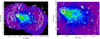 |
Fig. 6. Left panel: XMM-Newton smoothed image in the 0.3−10 keV band of A3376. The red sectors represent the regions used for the temperature and abundance distributions. Cyan circles are the point sources removed, with enlarged radius for clarity purpose. White contours are VLA 1.4 GHz radio contours. The solid yellow and orange lines show the X-ray shocks and cold front position, respectively. Right panel: BCG2 and BCG1 are marked with blue and black crosses. The numbers label the regions used in the spectral fitting. |
In the spectral analysis of A3376 we use two different observations as listed in Table 1. Specifically, ObsI:0151900101 is used for regions one, two, and three, while ObsID:0504140101 is used for regions six and seven. In addition, both these observations are used for the overlapping regions four and five. The background modelling parameters for each of the observations are shown in Tables B.3 and B.4. We fit the spectra of the annular sectors centred on BCG2, located close to the X-ray peak emission at the eastern subcluster. We assume the column density as NHI = 4.84 × 1020 cm−2 (Willingale et al. 2013). The best-fit parameters (see Table C.3) are in good agreement with previous studies with the Suzaku satellite (Akamatsu et al. 2012; Urdampilleta et al. 2018).
The temperature distribution of A3376 (Fig. 7) shows a central region with an average temperature ∼4 keV out to the outer radii where an increase of the temperature is seen. It is associated to the post merger region behind the western X-ray shock as described by Urdampilleta et al. (2018). The Fe abundance profile shows a peak of ∼0.5 Z⊙ in the core, coincident with the BCG2. At larger distances, the abundance decreases smoothly to reach ∼0.3 Z⊙ in regions four, five, and six, including BCG1 and in the surrounding diffuse gas. The lower abundance value appears in the outermost region of the cluster before the X-ray shock.
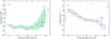 |
Fig. 7. Left panel: temperature distribution along the merging axis of A3376. Right panel: abundance distribution along the merging axis of A3376. The shadow area represent the systematic uncertainties. The shaded areas represent the systematic uncertainties: the green shadow correspond to the background normalisation variation, and the blue one to the temperature structure. The shaded grey areas show the cold front and radio relic position. The dashed shows the outer edge of the core spectral extraction region. The numbers and BCG1 blue point correspond to the regions and the red circle centred on BCG1, respectively shown in Fig. 6. |
4.4. A3667
Abell 3667 (hereafter A3667) is a widely studied bright, low redshift (z = 0.0553) and bimodal merging galaxy cluster (Markevitch et al. 1999). As a consequence of a violent merger along the northwest (NW) direction, A3667 hosts two curved radio relics to the NW and SE (Röttgering et al. 1997; Johnston-Hollitt 2003; Johnston-Hollitt & Pratley 2017; Carretti et al. 2013; Hindson et al. 2014; Riseley et al. 2015). The inner central region shows an elongated morphology of high-abundance gas in SE-NW direction (Mazzotta et al. 2002; Briel et al. 2004; Lovisari et al. 2009) according to the subcluster infall direction. A3667 also includes a prominent mushroom-like cold front close to the centre at SE (Vikhlinin et al. 2001; Briel et al. 2004; Owers et al. 2009; Datta et al. 2014; Ichinohe et al. 2017).
We fit the cluster emission and the background spectra (see Table B.5) in the elliptical regions as shown in Fig. 8, excluding the point sources and using NHI = 4.44 × 1020 cm−2 (Willingale et al. 2013). We use as centroid the main BCG ( ,
,  ), which is close to the X-ray emission peak (
 ,
,  ). We distribute the elliptical sectors along the merging axis assuming the BCG as the centre and following the X-ray morphology described by Briel et al. (2004).
The best-fit parameters are summarised in Table C.4 and represented in the distributions along the merging axis in Fig. 9. The results are in good agreement with previous studies (Briel et al. 2004; Lovisari et al. 2009; Akamatsu et al. 2013; Datta et al. 2014; Ichinohe et al. 2017). The distributions show a clear temperature decrease towards the cold front at SE. It has an opposite trend with the Fe abundance, which reaches a peak just behind the cold front. The value presented here is lower than the maximum found by Briel et al. (2004) and Lovisari et al. (2009) of ∼0.7 Z⊙, probably because our value includes larger azimuthal angles with lower abundance. However, if we select a smaller region in sector two (yellow dashed lines in Fig. 8), the temperature drops to 3.77 ± 0.09 keV and the abundance increases up to 0.64 ± 0.06 Z⊙. As pointed out by Lovisari et al. (2009), this behaviour agrees with the simulations of Heinz et al. (2003), which suggest a possible displacement of the central rich and cold gas of the subcluster centre well to the front during the infall, due to the internal dynamics of the cold front. The sectors in the NW direction (six to nine) show a temperature distribution close to ∼7 keV, meaning the average temperature of the cluster (Markevitch et al. 1999), and consistent with the hot tail described by Briel et al. (2004). The abundance in the central regions (two to four) is almost uniform, around ∼0.4 Z⊙, but higher than the main cluster value (∼0.2−0.3 Z⊙). Finally, the abundance is again flat in the outermost regions (seven to eight) close to ∼0.3 Z⊙.
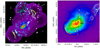 |
Fig. 8. Left panel: XMM-Newton smoothed image in the 0.3−10 keV band of A3667. The red elliptical sectors represent the regions used for the temperature and abundance distributions. The green sector is the offset region used for the sky background estimation. Cyan circles are the point sources removed, with enlarged radius for clarity purpose. White contours are SUMSS radio contours. The solid yellow and orange lines show the X-ray shocks and cold front position, respectively. Right panel: enlarged image of A3667. The BCG is marked with black cross. The solid orange line shows the cold front position. In addition to sector 2, the dashed yellow sector corresponds to a region considered also separately (see text). The numbers label the regions used in the spectral fitting. |
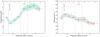 |
Fig. 9. Left panel: temperature distribution along the merging axis of A3667. Right panel: abundance distribution along the merging axis of A3667. The shaded areas represent the systematic uncertainties: green and orange shadows correspond to the background normalisation variation, and the blue one to the temperature structure. The shaded grey area shows the cold front position. The dashed lines show the outer edges of the core spectral extraction region. The numbers correspond to the regions shown in Fig. 8. |
4.5. A665
The two-body merging cluster Abell 665 (hereafter A665) was discovered as a non-relaxed cluster in an optical observation of Geller & Beers (1982). The authors found the first evidence of an elongated morphology and non-relaxed galaxy cluster. A665 is a hot cluster with an average temperature of ∼8.3 keV (Hughes & Tanaka 1992) and located at z = 0.182 (Gomez et al. 2000). The N-body hydrodynamical simulations and dynamic studies of Gomez et al. (2000) suggest a subcluster merger in the NW–SE direction with two similar masses. The bright core of the infalling subcluster is moving south, crossing a more diffuse halo, before being stripped by ram pressure. A665 hosts a giant radio halo (Jones & Saunders 1996; Feretti et al. 2004; Vacca et al. 2010), which follows the X-ray emission elongation. The X-ray observations of A665 (Markevitch & Vikhlinin 2001; Govoni et al. 2004; Dasadia et al. 2016) have revealed only one X-ray peak ( ,
,  ), close to the BCG, which indicates that only the infalling cluster core has survived the merger. The remnant core presents a nearby cold front in the SE, followed by a hot gas (∼8−15 keV) thought to be a post-merger region of a shock (Markevitch & Vikhlinin 2001; Govoni et al. 2004).
We use spectra from MOS, the only detector available for these observations, to fit the cluster emission together with the modelled background (Table B.6). We analyse the circular sectors centred on the BCG ( ,
,  ) as shown in Fig. 10, using NHI = 4.31 × 1020 cm−2 (Willingale et al. 2013). The best-fit parameters are presented in the Table C.5 and plotted in Fig. 11.
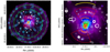 |
Fig. 10. Left panel: XMM-Newton smoothed image in the 0.3−10 keV band of A665. The red sectors represent the regions used for the temperature and abundance distributions. The green annulus is the offset region used for the sky background estimation. Cyan circles are the point sources removed, with enlarged radius for clarity purpose. White contours are VLA 1.4 GHz radio contours. Right panel: enlarged image of A665. The BCG is marked with a black cross. The magenta box includes the cooler gas region observed by Markevitch & Vikhlinin (2001). The solid yellow and orange lines show the X-ray shock and cold fronts position, respectively. The numbers label the regions used in the spectral fitting. |
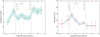 |
Fig. 11. Left panel: temperature distribution along the merging axis of A665. Right panel: abundance distribution along the merging axis of A665. The shaded area represent the systematic uncertainties: green shadow correspond to the background normalisation variation, and the blue one to the temperature structure. The shaded grey areas show the cold fronts position. The dashed lines show the outer edges of the core spectral extraction region. The numbers correspond to the regions shown in Fig. 10. |
The temperature and Fe abundance distributions along the merging axis show the presence of the two cold fronts as described by previous X-ray studies (Markevitch & Vikhlinin 2001; Govoni et al. 2004; Dasadia et al. 2016). We see a slight temperature decrease across them towards the centre. The abundance peak is found just within the south cold front and reflects the same case described by Heinz et al. (2003) for A3667. The diffuse gas in the north presents a lower abundance and a more uniform distribution (∼0.2−0.3 Z⊙) than the gas in the core and just behind the cold front in the south. This could indicate that the gas belongs to the more diffuse cluster, which had been already disrupted by the core-crossing. The two cold fronts seem to delimit a central region with a lower temperature (∼7 keV) than the surrounding gas. We found as well the cooler gas region (kT = 7.4 ± 0.2, Z = 0.33 ± 0.06 Z⊙) in the north observed by Markevitch & Vikhlinin (2001) and shown in Fig. 10 as a magenta box. This cooler region seems to belong to the infalling cluster coming from the NW direction as described by Markevitch & Vikhlinin (2001) and Govoni et al. (2004).
4.6. A2256
Abell 2256 (hereafter A2256) is a nearby (z = 0.058) rich galaxy cluster with bright X-ray emission. Optical analyses (Fabricant et al. 1989; Berrington et al. 2002; Miller et al. 2003) revealed a complex dynamical state, which consists of at least a triple merging with a mass ratio of 3:1:0.3. Berrington et al. (2002) propose that the system includes a main cluster with an infalling subcluster NW at ∼0.2 Gyr from the core passage (Roettiger et al. 1995) and another infalling group northeast (NE), possibly associated to a previous merger. Briel et al. (1991) detected two separate X-ray peaks corresponding to the main cluster and the infalling subcluster, lately confirmed by Sun et al. (2002) and Bourdin & Mazzotta (2008). They also found bimodality in the temperature structure along the cluster elongation axis, being the low temperature component (∼4.5 keV) associated with the subcluster and the higher temperature component (∼7−8 keV) with the main cluster. In addition, Tamura et al. (2011) found bulk motion of gas of the cooler temperature component.
We use two observations (see Table 1) for the analysis of A2256. We divide the ICM emission region in circular sectors along the cluster major elongation axis centred in the X-ray peak of the main cluster (CORE1:  ,
,  , Bourdin & Mazzotta 2008). We fit the cluster emission and the background spectra (see Tables B.7 and B.8) using NHI = 4.24 × 1020 cm−2 (Willingale et al. 2013). The best-fit parameters are presented in the Table C.6 and plotted in Fig. 13.
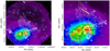 |
Fig. 12. Left panel: XMM-Newton smoothed image in the 0.3−10 keV band of A2256. The red sectors represent the regions used for the temperature and abundance distributions. The green sector is the offset region used for the sky background estimation. Cyan circles are the point sources removed, with enlarged radius for clarity purpose. White contours are WRST radio contours. Right panel: enlarged image of A2256. The CORE1 and CORE2 are marked with a black and blue crosses, respectively. The solid yellow and orange lines show the X-ray shocks and cold front position. The numbers label the regions used in the spectral fitting. |
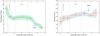 |
Fig. 13. Left panel: temperature distribution along the merging axis of A2256. Right panel: abundance distribution along the merging axis of A2256. The shaded area represent the systematic uncertainties: green and orange shadows correspond to the background normalisation variation, and the blue one to the temperature structure. The shaded grey area shows the cold front position. The dashed lines show the outer edges of the core spectral extraction region. The numbers and CORE2 blue point correspond to the regions and the red circle centred on CORE2, respectively shown in Fig. 12. |
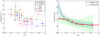 |
Fig. 14. Left panel: abundance distribution along the merging axis scaled by r500. Right panel: averaged abundance distribution scaled by r500. Data points in red show the averaged value and the statistical error as a thick errorbar plus the scatter as a thinner errorbar for each bin of Table 3. The blue shaded area shows the average profile for clusters (> 1.7 keV), including the statistical error and the scatter, derived by Mernier et al. (2017). The green shaded area represents the mean values for disturbed systems, together with the scatter, obtained by Lovisari & Reiprich (2019). The blue and green dashed line follow the average and mean abundance value of Mernier et al. (2017) and Lovisari & Reiprich (2019), respectively. |
The temperature profile shows the bimodal temperature structure already described by Sun et al. (2002) and Bourdin & Mazzotta (2008), as well as the hot (∼9 keV) temperature component south of the cluster centre. It shows a temperature discontinuity from the adjacent region at ∼7 keV, suggested to be caused by the presence of a cold front (Bourdin & Mazzotta 2008). However, and similarly to Bourdin & Mazzotta (2008), we do not find evidence for the presence of the “shoulder” mentioned by Sun et al. (2002) east of the CORE1. The Fe abundance distribution is in agreement with the values obtained by Sun et al. (2002). We obtain a quasi uniform abundance distribution (0.3−0.5 Z⊙) with a slight decrease at the south. The second X-ray peak, (CORE2:  ,
,  , Sun et al. 2002), associated to the infalling subcluster, presents the highest abundance value of ∼0.6 Z⊙.
5. Discussion
5.1. Averaged abundance distribution
The individual Fe abundance distributions of the six merging galaxy clusters along their merging axis are compiled in Fig. 14 (left). We remind the reader that such distributions are not azimuthally averaged. Instead, in this work we have chosen to trace the central ICM elongation along the merging axis, essentially because the surface brightness allows better constraints on the Fe abundance and because no spectacular metal redistribution is expected to take place perpendicular to the merging axis. In the case of CIZA2242, 1RXSJ0603 and A3376 the interest region clearly extends the core (where the BCG resides) to the outwards direction. For A3667, A665 and A2256, sectors along two opposite directions from the core are used. In Fig. 14, all the clustercentric radii have been rescaled to fractions of r500 5, adopting r500 and r200 values found in the literature and assuming the conversion r500 ≃ 0.65r200 of Reiprich et al. (2013). For our cosmology and redshifts we use the approximation of Henry et al. (2009):
 (1)
(1)
where E(z) = (ΩM(1 + z)3 + 1 − ΩM)1/2. The mean temperature values, ⟨kT⟩, are adopted from references as described in Table 2. Our averaged Fe abundance distribution, stacked from all the above measurements, is shown in Fig. 14 (right), and the numerical values are reported in Table 3.
Averaged abundance profile.
We use the stacking method of Mernier et al. (2017) to determine this distribution. The averaged abundance distribution, Zref(k), as a function of the kth reference bin is defined as:
 (2)
(2)
where Z(i)j is the individual abundance of the jth cluster at its ith region; σZ(i)j is its statistical error, N is the number of clusters, M is the number of regions analysed in each cluster and wi, j, k is the weighting factor. This factor represents the geometrical overlap of the ith region with the kth reference bin in cluster j. It varies from 0 to 1. The stacked statistical error is calculated as:
 (3)
(3)
We also obtained the scatter of the measurements for each kth reference bin as:
 (4)
(4)
It clearly appears from Fig. 14 that abundance distributions of these merging clusters are not flat. Instead, we note a decrease from the core up to ∼0.4r500, followed by a flattening at larger radii. Figure 14 (right) compares our averaged distribution with the relaxed, azimuthally-averaged CC systems of Mernier et al. (2017) with kT > 1.7 keV and the disturbed, NCC systems of Lovisari & Reiprich (2019). In both cases we have included the statistical errors and the scatter. Remarkably, our values are in good agreement with the (azimuthally-averaged) NCC profile of Lovisari & Reiprich (2019), which shows lower abundance values in the core than relaxed clusters and a shallower decrease towards the outer radii. The averaged Fe distribution values shown in Table 3 are therefore consistent with Lovisari & Reiprich (2019) results. We have additionally checked the averaged abundance distribution along the BCG displacement direction (assuming only the positive radii). In this case, the agreement with the NCC systems profile of Lovisari & Reiprich (2019) improves. For more details see Appendix A.
The lower abundance value in the core for disturbed systems is suggested by Lovisari & Reiprich (2019) to be caused by major mergers, where in some cases the core could be disrupted. As a result, the abundance peak in the centre of the (CC) progenitors is spread out and distributed across larger radii. At first glance, the similarity of the Fe distribution observed between NCC clusters and these merging clusters tends to support this scenario. However, the steeper Fe peaks observed in the core of 1RXSJ0603 and in the vicinity of the core of A665 (perhaps offset from the BCG because of important sloshing motions) suggest that remnants of previous CC clusters can partly persist to (or, at least, not be entirely disrupted by) even the most major mergers in some cases (see Sect. 5.2). While this moderate central abundance increase could be associated with either (relatively old) core passage mergers, or on the contrary, early stage mergers, we note that our sample contains both cases. In fact, most of them are massive clusters, which have undergone a major merger with a core passage more than 0.6 Gyr ago. However, A2256 is a still on going merger, before core passage, although it is thought that the main cluster centre is already affected by an older merger. Future larger samples, containing an equal proportion of early and late stage mergers, will help to relate the (re)-distribution of metals with merger history.
5.2. Abundance vs. pseudo-entropy relation
In order to study the thermal history of the ICM, we calculate the pseudo-entropy, K ≡ kT × n−2/3, as a function of the region distance for each merging cluster. These pseudo-entropy distributions along the merging axis are shown together with the Fe abundance profiles in Fig. 15. The temperature of each region, kT, is directly obtained from the spectral analysis, and the density, n, can be inferred from the emission measure, Norm, as Norm ∝ 1.2n2V, where V is the emitting volume projected onto the line-of-sight (LOS). To estimate n, we assume a spherical LOS in which only the sphere between the maximum and minimum radius contributes to the emission (Henry et al. 2004; Mahdavi et al. 2005). We assume the emission volume V to be V = 2SL/3 for the circular and elliptical sectors, and V = πSL/2 for rectangular ones. In each case,  and S is the area of the sectors in the plane of the sky.
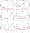 |
Fig. 15. Scaled pseudo-entropy (K/1000) and abundance distributions along the merging axis for CIZA2242, 1RXSJ0603, A3376, A3667, A665 and A2256. Dashed lines show the values of the yellow region after the A3667 cold front (see Fig. 8) and the CORE2 values of A2256 (see Fig. 12). |
Previous studies (De Grandi et al. 2004; Leccardi et al. 2010; Ghizzardi et al. 2014; Liu et al. 2018) have demonstrated, especially for relaxed (CC) clusters, the existence of a negative correlation between the Fe abundance and the gas entropy. Low-entropy cores, where the cooling of the ICM might take place, are in fact associated with central abundance peaks. However, disturbed (NCC) clusters are not well characterised by this behaviour as mentioned by Leccardi et al. (2010) and Rossetti & Molendi (2010).
Pseudo-entropy quantifies the internal energy variation due to thermal processes such as, for example cooling, turbulent dissipation or shock heating. Regions under the influence of the latter, in particular, can be easily identified because they exhibit a positive gradient proportional to r1.1 (Tozzi & Norman 2001). In particular for our merging cluster selection, we observe a similar trend in the post-shock regions, see Figs. 15 and 16 (left), although some systems (e.g. 1RXSJ0603, A3376) significantly deviate from this relation. If we fit simultaneously all our pseudo-entropy distributions with a power-law (∼rα), we obtain a slope of α = 1.34 ± 0.63 (Fig. 16 left). In the case of 1RXSJ0603, we see a flat profile between ∼0.2 and 0.4r500, coincident with the COREN location, possibly indicating a sign of the subcluster core remnant after the merger event. A similar flattening is observed in A3376, although its origin may be rather related to the central low-entropy gas stripped during the merger, thereby forming the cometary shape ICM.
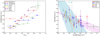 |
Fig. 16. Left panel: pseudo-entropy distribution scaled by r500. Right panel: distribution of Fe abundance versus the scaled pseudo-entropy of all the measured regions of the clusters: CIZA2242, 1RXSJ0603, A3376, A3667, A665 and A2256. The magenta dashed line is the best-fit linear model and the shaded area shows the 1σ uncertainties of the best-fit parameter. The cyan line and shadow are the results of Liu et al. (2018) for relaxed galaxy clusters. |
Most of NCC clusters are thought to have undergone a CC phase, before the (cool) core being disrupted completely or partially by major mergers (Leccardi et al. 2010; Rossetti & Molendi 2010; ZuHone 2011). The on-going interactions heat and increase the entropy in the core. Therefore, NCC tend to have high-entropy cores and smaller entropy gradients. Some of these clusters present regions with lower entropy that have associated an abundance excess, in most of the cases associated with the BCG or a giant elliptical galaxy, and known as “CC-remnants” (Rossetti & Molendi 2010). It is suggested that these regions are the reminiscent of CC after the merging activity. Another consequence of merger events is the decrease of the abundance excess in the core, which can be erased by the shock-heating and gas mixing processes.
Figure 15 shows simultaneously the pseudo-entropy and Fe abundance distributions scaled by r500 for our six merging galaxy clusters. In the case of CIZA2242 and A3376, the entropy is slightly flat in the core and the profile increases smoothly (though with a larger gradient) out to the recently shocked region. Interestingly, 1RXSJ0603 exhibits a relative low-entropy core associated with the abundance peak. One natural interpretation is that this region is the remainder of cool core after the merging activity, which agrees with ZuHone (2011) simulations taking into account the mass ratio of 3:1 and it is found in twelve clusters of Rossetti & Molendi (2010). An alternative scenario could be that 1RXSJ0603, as a well evolved merger (∼2 Gyr since the shock producing the radio relic; e.g. Brüggen et al. 2012, Stroe et al. 2015), has started to recover its potential well and to re-build its entropy (and metal) stratification after the merger. For A3667 and A2256, we identify possible CC-remnants characterised by somewhat lower entropy and higher metallicity values (Rossetti & Molendi 2010). These remnants clearly appear after we include the measurements of the truncated yellow region after the A3667 cold front (see Fig. 8) and the CORE2 values of A2256 (see Fig. 12), in dashed lines in Fig. 15. A2256 also contains a second minimum corresponding to the CORE1. As explained in Leccardi et al. (2010), two low-entropy clumps can be found if we are in the presence of an early stage merger, as in this case, or an off-axis merger event. A665 also shows a relative low-entropy drop in the core, but in this case the abundance peak is displaced towards the cold front, as explained in Sect. 5.1, possibly due to the effect of the internal dynamics of the cold front during the infall of the subcluster. The above examples, and in particular the case of 1RXSJ0603, strongly suggest that in some cases, signatures of cool cores can remain even after the most major ICM merger events.
Best-fit parameters of abundance vs pseudo-entropy distributions.
Furthermore, we try to determine a correlation between Fe abundance and pseudo-entropy for our merging clusters. Figure 16 (right) shows the distribution of Z–K. Generally speaking, our measured entropies are clearly higher than in the distribution of Liu et al. (2018), with our lowest value being ∼200 keV cm2 and the maximum abundance value being ∼0.5 Z⊙. In fact, these values are characteristic of merging clusters (Leccardi et al. 2010; ZuHone 2011). We fit the distribution with a linear function Z ∼ Z0 − α K/1000. Our best-fit parameters are Z0 = 0.51 ± 0.03 and α = 0.32 ± 0.06. This correlation shows a flatter slope than obtained by Liu et al. (2018) for relaxed (CC) galaxy clusters (Z0 = 0.86 ± 0.18 and α = 1.49 ± 0.51). Our results suggest that the abundance and pseudo-entropy relation are not always tightly related. Instead, it is likely that, when a merger occurs, the entropy gets boosted in post-shock regions more rapidly than metals diffuse out. Interestingly, when we consider the values of pseudo-entropy only below ∼500 keV cm2 – which were presumably less affected by shock-heating, or which start to relax again (see vertical black dashed line in Fig. 16), the slope of the relation considerably increases (Table 4). This might suggest that in the lowest entropy regions (∼200−500 keV cm2) of these merging clusters (NCC) – usually associated with the core remnant (see Fig. 15), the metal-rich gas (originally still coming from the BCG) gets mixed and redistributed at a moderate rate compared to the entropy changes during the merger event (ZuHone 2011). Alternatively, chemical histories may differ between relaxed and merging systems. Although beyond the scope of this paper, in some cases we cannot rule out the possibility of an extra Fe enrichment, produced by a boost of star formation or SNIa explosions, triggered by major mergers (e.g. Stroe et al. 2015; Sobral et al. 2015).
Finally, we do not find evidence of a correlation in the higher (> 500 keV cm2) entropy range, meaning beyond ∼0.4−0.6r500. In these outer regions, the Fe abundance remains rather uniform around 0.2−0.3 Z⊙, with no notable trend with cluster mass, radius or azimuth (Fig. 14). Combined with the previous observations of a uniform ∼0.3 Z⊙ Fe abundance in the outskirts of (mostly) CC clusters (Fujita et al. 2008; Werner et al. 2013; Thölken et al. 2016; Urban et al. 2017; Ezer et al. 2017), we conclude that Fe distribution in cluster outskirts of these merging clusters depends very weakly (or not at all) on the dynamical state of the cluster. This has important consequences regarding the chemical history of large-scale structures. In fact, although these previous measurements in relaxed systems strongly suggested that the most of the ICM enrichment took place in early stages of cluster formation (i.e. at z > 2−3; for recent reviews, see Mernier et al. 2018a; Biffi et al. 2018b), the alternative scenario of late enrichment coupled with a very efficient mixing of metals in the ICM, could not be totally excluded. Among the entire cluster population, merging clusters are systems in which metals had the least time to mix and diffuse out since their last merger event. Consequently, if the bulk of metals were mixed efficiently in the entire cluster volume (after being injected into the ICM at late stages), one would expect to find important variations of the Fe abundance at large radii in such dynamically disturbed systems, with values considerably higher than 0.2−0.3 Z⊙ in some specific outer regions. Instead, the remarkable similarity of the Fe distribution in the outskirts of CC and these six merging clusters, and the above indication that in inner regions metal mixing lags somewhat behind entropy changes, constitute valuable additional evidence in favour of the early enrichment scenario.
6. Summary
In this work, we analyse for the first time the Fe distribution along the merging axis of six merging galaxy clusters (0.05 < z < 0.23) observed with XMM-Newton/EPIC. We obtain and specifically studied the temperature, abundance and pseudo-entropy distributions across the ICM of these disturbed systems. Specifically, we provide a first estimate of the averaged Fe distribution out to r500 – as well as the relation between Fe abundance and pseudo-entropy – in six merging clusters. The main results can be summarised as follows.
Firstly, the Fe distribution is far from being universal, as it strongly varies from one merging cluster to another. While in some cases (e.g. CIZA2242, A2256) no Fe peak nor pseudo-entropy drop is detected in central regions, some of our observations (e.g. 1RXSJ0603, A665) strongly suggest that remnants of previous (metal-rich) cool-cores can persist after major mergers.
Secondly, our averaged Fe distribution in these six merging clusters is in excellent agreement with that in (non-merging) non-cool-core clusters presented by Lovisari & Reiprich (2019). The average profile clearly shows a moderate abundance central excess, thus present not only in CC systems but even in many spectacular mergers. Compared to the former, however, the central (≲0.3r500) Fe profile in these merging clusters is significantly less steep. This can be interpreted as the metal-rich gas of the CC progenitors being mixed and spread across moderate radii by merging processes.
Thirdly, the minimum pseudo-entropy value obtained for these six merging clusters is ∼200 keV cm2. This value is characteristic of typical unrelaxed systems, whose internal activity is dominated by turbulence, large-scale motions and/or AGN feedback. Whereas some clusters exhibit a pseudo-entropy distribution that tends to follow the behaviour ∝r1.1 described by Tozzi & Norman (2001), some systems (e.g. 1RXSJ0603, A3376) deviate from this relation due to stripped cold gas from disrupted cores.
Fourthly, we find a mild negative correlation between abundance and pseudo-entropy for the inner core region (K = 200−500 keV cm2), shallower than the anti-correlation obtained by Liu et al. (2018) for relaxed clusters. This might suggest that mergers affect the gas entropy more rapidly than they re-distribute metals (via gas mixing).
Finally, in the outermost, high-entropy regions (K = 500−2300 keV cm2) studied here, we have no evidence of a correlation between metallicity and pseudo-entropy and the abundance is consistent with the uniform abundance value of 0.2−0.3 Z⊙. This demonstrates that the lack of dependence of Fe abundance at such high entropies (and large radii) applies not only to the mass, radius and azimuthal characteristics of clusters, but also to the dynamical stage. In other words, our results provide important additional evidence towards the scenario of an early enrichment of the inter galactic medium (z > 2−3).
It should be noted that the flux of the faintest resolved and excluded point source, and hence the remaining unresolved CXB flux, depend on the exposure time. In our case, most of the observations have similar a exposure except two: 0151900101 and 0653050201. Even for these data sets, the SP power law norm is free to vary and will compensate for any residuals in the CXB subtraction.
rΔ is formally defined as the radius within which the density is Δ times the critical density of the Universe at the redshift of the source.
Acknowledgments
The authors thank Dr. R. van Weeren for the LOFAR radio data, Dr. R. Kale, Dr. T. Shimwell and Dr. V. Vacca for providing the VLA radio data and Dr. A. Botteon for the SUMMSS data. S. Kara and E. N. Ercan would like to thank TUBITAK for financial support through a 1002 project under the code 118F023. A. Simionescu is supported by the Women In Science Excel (WISE) programme of the Netherlands Organisation for Scientific Research (NWO), and acknowledges the MEXT World Premier Research Center Initiative (WPI) and the Kavli IPMU for the continued hospitality. SRON is supported financially by NWO, the Netherlands Organization for Scientific Research. This work is based on observations obtained with XMM-Newton, an ESA science mission with instruments and contributions directly funded by ESA member states and the USA (NASA).
References
- Akamatsu, H., Takizawa, M., Nakazawa, K., et al. 2012, PASJ, 64 [Google Scholar]
- Akamatsu, H., Inoue, S., Sato, T., et al. 2013, PASJ, 65, 89 [NASA ADS] [Google Scholar]
- Akamatsu, H., van Weeren, R. J., Ogrean, G. A., et al. 2015, A&A, 582, A20 [Google Scholar]
- Bagchi, J., Durret, F., Lima Neto, G. B., & Paul, S. 2006, Science, 314, 791 [NASA ADS] [CrossRef] [PubMed] [Google Scholar]
- Baldi, A., Ettori, S., Mazzotta, P., Tozzi, P., & Borgani, S. 2007, ApJ, 666, 835 [NASA ADS] [CrossRef] [Google Scholar]
- Baumgartner, V., & Breitschwerdt, D. 2009, Astron. Nachr., 330, 898 [NASA ADS] [CrossRef] [Google Scholar]
- Bell, A. R. 1987, MNRAS, 225, 615 [NASA ADS] [Google Scholar]
- Berrington, R. C., Lugger, P. M., & Cohn, H. N. 2002, AJ, 123, 2261 [NASA ADS] [CrossRef] [Google Scholar]
- Biffi, V., Planelles, S., Borgani, S., et al. 2017, MNRAS, 468, 531 [NASA ADS] [CrossRef] [Google Scholar]
- Biffi, V., Planelles, S., Borgani, S., et al. 2018a, MNRAS, 476, 2689 [NASA ADS] [CrossRef] [Google Scholar]
- Biffi, V., Mernier, F., & Medvedev, P. 2018b, Space Sci. Rev., 214, 123 [NASA ADS] [CrossRef] [Google Scholar]
- Blandford, R., & Eichler, D. 1987, Phys. Rep., 154, 1 [Google Scholar]
- Böhringer, H., & Werner, N. 2010, A&ARv, 18, 127 [NASA ADS] [CrossRef] [Google Scholar]
- Bourdin, H., & Mazzotta, P. 2008, A&A, 479, 307 [NASA ADS] [CrossRef] [EDP Sciences] [Google Scholar]
- Bridle, A. H., & Fomalont, E. B. 1976, A&A, 52, 107 [NASA ADS] [Google Scholar]
- Briel, U. G., Herny, J. P., Schwarz, R. A., et al. 1991, A&A, 246, L10 [NASA ADS] [Google Scholar]
- Briel, U. G., Finoguenov, A., & Henry, J. P. 2004, A&A, 426, 1 [NASA ADS] [CrossRef] [EDP Sciences] [Google Scholar]
- Brüggen, M., van Weeren, R. J., & Röttgering, H. J. 2012, MNRAS, 425, L76 [NASA ADS] [CrossRef] [Google Scholar]
- Brunetti, G., & Jones, T. W. 2014, Int. J. Mod. Phys. D, 23, 1430007 [Google Scholar]
- Brunetti, G., Setti, G., Feretti, L., & Giovannini, G. 2001, MNRAS, 320, 365 [NASA ADS] [CrossRef] [Google Scholar]
- Buote, D. A. 2000, MNRAS, 311, 176 [NASA ADS] [CrossRef] [Google Scholar]
- Carretti, E., Brown, S., Staveley-Smith, L., et al. 2013, MNRAS, 430, 1414 [NASA ADS] [CrossRef] [Google Scholar]
- Cash, W. 1979, ApJ, 228, 939 [NASA ADS] [CrossRef] [Google Scholar]
- Clarke, T. E., & Ensslin, T. A. 2006, ApJ, 131, 2900 [NASA ADS] [CrossRef] [Google Scholar]
- Dasadia, S., Sun, M., Sarazin, C., et al. 2016, ApJ, 820, L20 [Google Scholar]
- Datta, A., Schenck, D. E., Burns, J. O., Skillman, S. W., & Hallman, E. J. 2014, ApJ, 793, 80 [NASA ADS] [CrossRef] [Google Scholar]
- Dawson, W. A., Jee, M. J., Stroe, A., et al. 2015, ApJ, 805, 143 [NASA ADS] [CrossRef] [Google Scholar]
- De Luca, A., & Molendi, S. 2004, A&A, 419, 837 [NASA ADS] [CrossRef] [EDP Sciences] [Google Scholar]
- De Grandi, S., & Molendi, S. 2001, ApJ, 551, 153 [NASA ADS] [CrossRef] [Google Scholar]
- De Grandi, S., Ettori, S., Longhetti, M., & Molendi, S. 2004, A&A, 419, 7 [NASA ADS] [CrossRef] [EDP Sciences] [Google Scholar]
- de Plaa, J. 2013, Astron. Nachr., 334, 416 [NASA ADS] [CrossRef] [Google Scholar]
- de Plaa, J. 2017, https://doi.org/10.5281/zenodo.2575495 [Google Scholar]
- de Plaa, J., Werner, N., Bykov, A. M., et al. 2006, A&A, 452, 397 [NASA ADS] [CrossRef] [EDP Sciences] [Google Scholar]
- Durret, F., Perrot, C., Lima Neto, G. B., et al. 2013, A&A, 560, A78 [NASA ADS] [CrossRef] [EDP Sciences] [Google Scholar]
- Elkholy, T. Y., Bautz, M. W., & Canizares, C. R. 2015, ApJ, 805, 3 [NASA ADS] [CrossRef] [Google Scholar]
- Ettori, S., Ghirardini, V., Eckert, D., Dubath, F., & Pointecouteau, E. 2017, MNRAS, 470, L29 [NASA ADS] [CrossRef] [Google Scholar]
- Ezer, C., Bulbul, E., Nihal Ercan, E., et al. 2017, ApJ, 836, 110 [NASA ADS] [CrossRef] [Google Scholar]
- Fabricant, D. G., Kent, S. M., & Kurtz, M. J. 1989, ApJ, 336, 77 [NASA ADS] [CrossRef] [Google Scholar]
- Feretti, L., Orrù, E., Brunetti, G., et al. 2004, A&A, 423, 111 [NASA ADS] [CrossRef] [EDP Sciences] [Google Scholar]
- Feretti, L., Giovannini, G., Govoni, F., & Murgia, M. 2012, A&ARv, 20, 54 [Google Scholar]
- Ferrari, C., Govoni, F., Schindler, S., Bykov, A. M., & Rephaeli, Y. 2008, Space Sci. Rev., 134, 93 [NASA ADS] [CrossRef] [Google Scholar]
- Fujita, Y., Tawa, N., Hayashida, K., et al. 2008, PASJ, 60, 343 [Google Scholar]
- Geller, M. J., & Beers, T. C. 1982, PASP, 94, 421 [NASA ADS] [CrossRef] [Google Scholar]
- Ghizzardi, S., De Grandi, S., & Molendi, S. 2014, A&A, 570, A117 [NASA ADS] [CrossRef] [EDP Sciences] [Google Scholar]
- Gomez, P. L., Hughes, J. P., & Birkinshaw, M. 2000, ApJ, 540, 726 [NASA ADS] [CrossRef] [Google Scholar]
- Govoni, F., Markevitch, M., Vikhlinin, A., et al. 2004, ApJ, 605, 695 [NASA ADS] [CrossRef] [Google Scholar]
- Heinz, S., Churazov, E., Forman, W., Jones, C., & Briel, U. G. 2003, MNRAS, 346, 13 [Google Scholar]
- Henry, J. P., Finoguenov, A., & Briel, U. G. 2004, ApJ, 615, 181 [NASA ADS] [CrossRef] [Google Scholar]
- Henry, J. P., Evrard, A. E., Hoekstra, H., Babul, A., & Mahdavi, A. 2009, ApJ, 691, 1307 [NASA ADS] [CrossRef] [Google Scholar]
- Hindson, L., Johnston-Hollitt, M., Hurley-Walker, N., et al. 2014, MNRAS, 445, 330 [NASA ADS] [CrossRef] [Google Scholar]
- Hitomi Collaboration (Aharonian, F., et al.) 2018, PASJ, 70, 12 [NASA ADS] [Google Scholar]
- Hopkins, A. M., & Beacom, J. F. 2006, ApJ, 651, 142 [NASA ADS] [CrossRef] [MathSciNet] [Google Scholar]
- Hughes, J. P., & Tanaka, Y. 1992, ApJ, 398, 62 [NASA ADS] [CrossRef] [Google Scholar]
- Ichinohe, Y., Simionescu, A., Werner, N., & Takahashi, T. 2017, MNRAS, 467, 3662 [NASA ADS] [CrossRef] [Google Scholar]
- Itahana, M., Takizawa, M., Akamatsu, H., et al. 2015, PASJ, 67, 1 [Google Scholar]
- Jee, M. J., Stroe, A., Dawson, W., et al. 2015, ApJ, 802, 46 [NASA ADS] [CrossRef] [Google Scholar]
- Jee, M. J., Dawson, W. A., Stroe, A., et al. 2016, ApJ, 817, 179 [NASA ADS] [CrossRef] [Google Scholar]
- Johnston-Hollitt, M. 2003, PhD Thesis, University of Adelaide, Australia [Google Scholar]
- Johnston-Hollitt, M., & Pratley, L. 2017, ArXiv e-prints [arXiv:1706.04930] [Google Scholar]
- Jones, M., & Saunders, R. 1996, Röntgenstrahlung from the Universe, MPE Report 263, 553 [Google Scholar]
- Kaastra, J. S. 2017, A&A, 605, A51 [NASA ADS] [CrossRef] [EDP Sciences] [Google Scholar]
- Kaastra, J. S., & Bleeker, J. A. M. 2016, A&A, 587, A151 [NASA ADS] [CrossRef] [EDP Sciences] [Google Scholar]
- Kaastra, J. S., Mewe, R., & Nieuwenhuijzen, H. 1996, 11th Colloquium on UV and X-ray Spectroscopy of Astrophysical and Laboratory Plasmas, 411 [Google Scholar]
- Kaastra, J. S., Tamura, T., Peterson, J. R., et al. 2004, A&A, 413, 415 [NASA ADS] [CrossRef] [EDP Sciences] [Google Scholar]
- Kaastra, J. S., Raassen, A. J. J., de Plaa, J., & Gu, L. 2017, https://doi.org/10.5281/zenodo.2272992 [Google Scholar]
- Kale, R., Dwarakanath, K. S., Bagchi, J., & Paul, S. 2012, MNRAS, 426, 1204 [NASA ADS] [CrossRef] [Google Scholar]
- Kapferer, W., Ferrari, C., Domainko, W., et al. 2006, A&A, 447, 827 [NASA ADS] [CrossRef] [EDP Sciences] [Google Scholar]
- Kapferer, W., Kronberger, T., Weratschnig, J., et al. 2007, A&A, 466, 813 [NASA ADS] [CrossRef] [EDP Sciences] [Google Scholar]
- Kapferer, W., Kronberger, T., Breitschwerdt, D., et al. 2009, A&A, 504, 719 [NASA ADS] [CrossRef] [EDP Sciences] [Google Scholar]
- Kocevski, D. D., Ebeling, H., Mullis, C. R., & Tully, R. B. 2007, ApJ, 662, 224 [NASA ADS] [CrossRef] [Google Scholar]
- Laganá, T. F., Durret, F., & Lopes, P. A. A. 2019, MNRAS, 484, 2807 [NASA ADS] [CrossRef] [Google Scholar]
- Leccardi, A., & Molendi, S. 2008, A&A, 487, 461 [NASA ADS] [CrossRef] [EDP Sciences] [Google Scholar]
- Leccardi, A., Rossetti, M., & Molendi, S. 2010, A&A, 510, A82 [NASA ADS] [CrossRef] [EDP Sciences] [Google Scholar]
- Liu, A., Tozzi, P., Yu, H., De Grandi, S., & Ettori, S. 2018, MNRAS, 481, 361 [NASA ADS] [CrossRef] [Google Scholar]
- Lodders, K., Palme, H., & Gail, H. P. 2009, Landolt Bömstein, New Series, Astronomy and Astrophysics (Springer Verlag), VI/4B, 560 [Google Scholar]
- Lovisari, L., & Reiprich, T. H. 2019, MNRAS, 483, 540 [NASA ADS] [CrossRef] [Google Scholar]
- Lovisari, L., Kapferer, W., Schindler, S., & Ferrari, C. 2009, A&A, 508, 191 [NASA ADS] [CrossRef] [EDP Sciences] [Google Scholar]
- Lumb, D. H., Warwick, R. S., Page, M., & De Luca, A. 2002, A&A, 389, 93 [NASA ADS] [CrossRef] [EDP Sciences] [Google Scholar]
- Machado, R. E. G., & Lima Neto, G. B. 2013, MNRAS, 430, 3249 [NASA ADS] [CrossRef] [Google Scholar]
- Madau, P., & Dickinson, M. 2014, ARA&A, 52, 415 [NASA ADS] [CrossRef] [Google Scholar]
- Mahdavi, A., Finoguenov, A., Böhringer, H., Geller, M. J., & Henry, J. P. 2005, ApJ, 622, 187 [Google Scholar]
- Mantz, A. B., Allen, S. W., Morris, R. G., et al. 2017, MNRAS, 472, 2877 [NASA ADS] [CrossRef] [Google Scholar]
- Markevitch, M., & Vikhlinin, A. 2001, ApJ, 563, 95 [NASA ADS] [CrossRef] [Google Scholar]
- Markevitch, M., & Vikhlinin, A. 2007, Phys. Rep., 443, 1 [NASA ADS] [CrossRef] [EDP Sciences] [Google Scholar]
- Markevitch, M., Sarazin, C. L., & Vikhlinin, A. 1999, ApJ, 521, 526 [Google Scholar]
- Matsushita, K. 2011, A&A, 527, A134 [NASA ADS] [CrossRef] [EDP Sciences] [Google Scholar]
- Maughan, B. J., Jones, C., Forman, W., & van Speybroeck, L. 2008, ApJS, 174, 117 [NASA ADS] [CrossRef] [Google Scholar]
- Mazzotta, P., Fusco-Femiano, R., & Vikhlinin, A. 2002, ApJ, 569, L31 [NASA ADS] [CrossRef] [Google Scholar]
- McDonald, M., Bulbul, E., de Haan, T., et al. 2016, ApJ, 826, 124 [NASA ADS] [CrossRef] [Google Scholar]
- Mernier, F., de Plaa, J., Lovisari, L., et al. 2015, A&A, 575, A37 [Google Scholar]
- Mernier, F., de Plaa, J., Pinto, C., et al. 2016, A&A, 595, A126 [NASA ADS] [CrossRef] [EDP Sciences] [Google Scholar]
- Mernier, F., de Plaa, J., Kaastra, J. S., et al. 2017, A&A, 603, A80 [NASA ADS] [CrossRef] [EDP Sciences] [Google Scholar]
- Mernier, F., Biffi, V., Yamaguchi, H., et al. 2018a, Space Sci. Rev., 214, 129 [NASA ADS] [CrossRef] [Google Scholar]
- Mernier, F., de Plaa, J., Werner, N., et al. 2018b, MNRAS, 478, L116 [NASA ADS] [CrossRef] [Google Scholar]
- Miller, N. A., Owen, F. N., & Hill, J. M. 2003, AJ, 125, 2393 [NASA ADS] [CrossRef] [Google Scholar]
- Moffet, A. T., & Birkinshaw, M. 1989, ApJ, 98, 1148 [Google Scholar]
- Monteiro-Oliveira, R., Neto, G. B. L., Cypriano, E. S., et al. 2017, MNRAS, 468, 4566 [NASA ADS] [CrossRef] [Google Scholar]
- Ogrean, G. A., Brüggen, M., van Weeren, R. J., et al. 2013a, MNRAS, 433, 812 [NASA ADS] [CrossRef] [Google Scholar]
- Ogrean, G., Brüggen, M., Simionescu, A., et al. 2013b, MNRAS, 429, 2617 [NASA ADS] [CrossRef] [Google Scholar]
- Ogrean, G. A., Brüggen, M., van Weeren, R., et al. 2014, MNRAS, 440, 3416 [NASA ADS] [CrossRef] [Google Scholar]
- Owers, M. S., Couch, W. J., & Nulsen, P. E. J. 2009, ApJ, 693, 901 [NASA ADS] [CrossRef] [Google Scholar]
- Paul, S., Iapichino, L., Miniati, F., Bagchi, J., & Mannheim, K. 2011, ApJ, 726, 17 [NASA ADS] [CrossRef] [Google Scholar]
- Rajpurohit, K., Hoeft, M., van Weeren, R. J., et al. 2018, ApJ, 852, 65 [NASA ADS] [CrossRef] [Google Scholar]
- Reiprich, T. H., Basu, K., Ettori, S., et al. 2013, Space Sci. Rev., 177, 195 [NASA ADS] [CrossRef] [EDP Sciences] [Google Scholar]
- Riseley, C. J., Scaife, A. M., Oozeer, N., Magnus, L., & Wise, M. W. 2015, MNRAS, 447, 1895 [NASA ADS] [CrossRef] [Google Scholar]
- Roettiger, K., Burns, J. O., & Pinkney, J. 1995, ApJ, 453, 634 [NASA ADS] [CrossRef] [Google Scholar]
- Roettiger, K., Burns, J. O., & Stone, J. M. 1999, ApJ, 518, 603 [NASA ADS] [CrossRef] [Google Scholar]
- Rossetti, M., & Molendi, S. 2010, A&A, 510, A83 [Google Scholar]
- Röttgering, H. J., Wieringa, M. H., Hunstead, R. W., & Ekers, R. D. 1997, MNRAS, 290, 577 [NASA ADS] [CrossRef] [Google Scholar]
- Rumsey, C., Perrott, Y. C., Olamaie, M., et al. 2017, MNRAS, 470, 4638 [NASA ADS] [CrossRef] [Google Scholar]
- Sarazin, C. L., Finoguenov, A., Wik, D. R., & Clarke, T. E. 2016, ApJ, submitted [arXiv:1606.07433] [Google Scholar]
- Schindler, S., Kapferer, W., Domainko, W., et al. 2005, A&A, 435, L25 [NASA ADS] [CrossRef] [EDP Sciences] [Google Scholar]
- Simionescu, A., Werner, N., Finoguenov, A., Böhringer, H., & Brüggen, M. 2008, A&A, 482, 97 [NASA ADS] [CrossRef] [EDP Sciences] [Google Scholar]
- Simionescu, A., Werner, N., Böhringer, H., et al. 2009, A&A, 493, 409 [NASA ADS] [CrossRef] [EDP Sciences] [Google Scholar]
- Simionescu, A., Werner, N., Forman, W. R., et al. 2010, MNRAS, 405, 91 [NASA ADS] [Google Scholar]
- Simionescu, A., Werner, N., Mantz, A., Allen, S. W., & Urban, O. 2017, MNRAS, 496, 1476 [NASA ADS] [CrossRef] [Google Scholar]
- Simionescu, A., Nakashima, S., Yamaguchi, H., et al. 2019, MNRAS, 483, 1701 [NASA ADS] [CrossRef] [Google Scholar]
- Sobral, D., Stroe, A., Dawson, W. A., et al. 2015, MNRAS, 450, 630 [NASA ADS] [CrossRef] [Google Scholar]
- Stroe, A., & Sobral, D. 2015, MNRAS, 453, 242 [NASA ADS] [CrossRef] [Google Scholar]
- Stroe, A., Harwood, J. J., Hardcastle, M. J., & Röttgering, H. J. 2014a, MNRAS, 445, 1213 [NASA ADS] [CrossRef] [Google Scholar]
- Stroe, A., Sobral, D., Röttgering, H. J., & van Weeren, R. J. 2014b, MNARS, 438, 1377 [Google Scholar]
- Stroe, A., Oosterloo, T., Röttgering, H. J., et al. 2015, MNARS, 452, 2731 [Google Scholar]
- Stroe, A., Sobral, D., Paulino-Afonso, A., et al. 2017, MNRAS, 465, 2916 [NASA ADS] [CrossRef] [Google Scholar]
- Sun, M., Murray, S. S., Markevitch, M., & Vikhlinin, A. 2002, ApJ, 565, 867 [NASA ADS] [CrossRef] [Google Scholar]
- Tamura, T., Hayashida, K., Ueda, S., & Nagai, M. 2011, PASJ, 63, S1009 [NASA ADS] [CrossRef] [Google Scholar]
- Thölken, S., Lovisari, L., Reiprich, T. H., & Hasenbusch, J. 2016, A&A, 592, A37 [NASA ADS] [CrossRef] [EDP Sciences] [Google Scholar]
- Tozzi, P., & Norman, C. 2001, ApJ, 546, 63 [NASA ADS] [CrossRef] [Google Scholar]
- Trasatti, M., Akamatsu, H., Lovisari, L., et al. 2015, A&A, 575, A45 [NASA ADS] [CrossRef] [EDP Sciences] [Google Scholar]
- Urban, O., Werner, N., Allen, S. W., Simionescu, A., & Mantz, A. 2017, MNRAS, 470, 4583 [NASA ADS] [CrossRef] [Google Scholar]
- Urdampilleta, I., Akamatsu, H., Mernier, F., et al. 2018, A&A, 618, A74 [NASA ADS] [CrossRef] [EDP Sciences] [Google Scholar]
- Vacca, V., Govoni, F., Murgia, M., et al. 2010, A&A, 541, A71 [CrossRef] [EDP Sciences] [Google Scholar]
- van Weeren, R. J., Rottgering, H. J. A., Bruggen, M., & Hoeft, M. 2010, Science, 330, 347 [NASA ADS] [CrossRef] [PubMed] [Google Scholar]
- van Weeren, R. J., Brüggen, M., Röttgering, H. J., & Hoeft, M. 2011, MNARS, 418, 230 [NASA ADS] [CrossRef] [Google Scholar]
- van Weeren, R. J., Röttgering, H. J. A., Intema, H. T., et al. 2012, A&A, 546, A124 [NASA ADS] [CrossRef] [EDP Sciences] [Google Scholar]
- van Weeren, R. J., Brunetti, G., Brüggen, M., et al. 2016, ApJ, 818, 204 [NASA ADS] [CrossRef] [Google Scholar]
- van Weeren, R. J., de Gasperin, F., Akamatsu, H., et al. 2019, Space Sci. Rev., 215, 16 [NASA ADS] [CrossRef] [Google Scholar]
- Vikhlinin, A., Markevitch, M., & Murray, S. S. 2001, ApJ, 551, 160 [NASA ADS] [CrossRef] [Google Scholar]
- Werner, N., Durret, F., Ohashi, T., Schindler, S., & Wiersma, R. P. C. 2008, Space Sci. Rev., 134, 337 [NASA ADS] [CrossRef] [Google Scholar]
- Werner, N., Urban, O., Simionescu, A., & Allen, S. W. 2013, Nature, 502, 656 [NASA ADS] [CrossRef] [Google Scholar]
- Willingale, R., Starling, R. L. C., Beardmore, A. P., Tanvir, N. R., & O’Brien, P. T. 2013, MNRAS, 431, 394 [NASA ADS] [CrossRef] [Google Scholar]
- ZuHone, J. A. 2011, ApJ, 728, 54 [NASA ADS] [CrossRef] [Google Scholar]
Appendix A: Averaged abundance distribution along BCG displacement direction
Averaged abundance distribution.
In addition to stacking our measurements over the entire merger axis as explained in Sect. 5.1, we can alternatively choose to trace the ICM only from the BCG region (i.e. typically including the cluster X-ray peak), down to the freshly collided gas, meaning along its cometary structure (defined in Figs. 3, 5, 7, 9, 11, and 13 as positive values on the x-axis). These regions better trace the disturbed and mixed plasma while avoiding special features such as cold fronts ahead of the merger (e.g. A3667, Fig. 9); therefore the effects of the merging activity in the ICM are expected to be more significant. For CIZA2242, 1RXSJ0603, and A3376 this covers the complete elongation or cometary tail present in the ICM. For A3367 and A665 this includes the sectors five to eight and four to nine, respectively. In the case of A2256, we consider the sectors four to seven, where the ICM of the main subclusters is predominantly affected by the presence of the infalling subclsuter. The individual Fe abundance distribution of the six merging galaxy clusters included in this analysis are plotted in Fig. A.1 (top), the averaged values obtained with the stacking method described in Sect. 5.1 are shown in Fig. A.1 (bottom) and Table A.1.
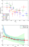 |
Fig. A.1. Top panel: abundance distribution along the BCG displacement direction scaled by r500. Bottom panel: averaged abundance distribution scaled by r500. Data points in red show the averaged value and the statistical error as a thick errorbar plus the scatter as a thinner errorbar for each bin of Table 3. The blue shaded area shows the average profile for clusters (> 1.7 keV), including the statistical error and the scatter, derived by Mernier et al. (2017). The green shaded area represents the mean values for disturbed systems, together with the scatter, obtained by Lovisari & Reiprich (2019). The blue and green dashed line follow the average and mean abundance value of Mernier et al. (2017) and Lovisari & Reiprich (2019), respectively. |
Interestingly, the Fe averaged distribution is now in excellent agreement with the Fe average profile of NCC systems by Lovisari & Reiprich (2019). The major differences with respect to the distribution shown in Sect. 5.1 appear in the 0.1−0.2r500 (8% lower) and 0.2−0.3r500 (10% lower) radii. These lower values are obtained because the displaced Fe peak outside cluster centre (see Sects. 5.1 and 5.2 for more details) of A3667 and A665 are not included.
Appendix B: EPIC background modelling for the cluster sample
The following tables summarise the EPIC background model parameters used of each one of the galaxy clusters using the method described in Sect. 3.2. The norms are given in standard SPEX definition, which are intrinsically dependent of the distance to the source.
Background components derived from the CIZA2242 observation.
Background components derived from the 1RXSJ0603 observation.
Best-fit parameter values of the total background estimated for A3376 E observation.
Best-fit parameter values of the total background estimated for A3376 W observation.
Background components derived from the A3667 observation.
Background components derived from the A665 observation.
Background components derived from the A2256 pointing 1 observation.
Background components derived from the A2256 pointing 2 observation.
Appendix C: Temperature and abundance analysis for the cluster sample
The following tables summarise the best-fit parameters for the temperature and abundance distribution along the merging axis.
Best-fit parameters for CIZA2242 regions shown in Fig. 2.
Best-fit parameters for 1RXSJ0603 regions shown in Fig. 4.
Best-fit parameters for A3376 regions shown in Fig. 6.
Best-fit parameters for A3667 regions shown in Fig. 8.
Best-fit parameters for A665 regions shown in Fig. 10.
Best-fit parameters for A2256 regions shown in Fig. 12.
All Tables
Best-fit parameter values of the total background estimated for A3376 E observation.
Best-fit parameter values of the total background estimated for A3376 W observation.
All Figures
|
Fig. 1. EPIC MOS2 spectrum of CIZA2242 core (r = 1.5′). The solid black line represents the best-fit model. The cluster emission ICM and all background components (LHB, MHW, CXB, HF, HP and SP) are also shown. |
| In the text | |
|
Fig. 2. Left panel: XMM-Newton smoothed image in the 0.3−10 keV band of CIZA2242. The red sectors represent the regions used for the radial temperature and abundance profiles. The green sector is the offset region used for the sky background estimation. Cyan circles are the point sources removed (with enlarged radius for clarity purpose). White contours are LOFAR radio contours. Right panel: enlarged image of CIZA2242. The BCGN and BCGS are marked with blue and black crosses, respectively. The solid yellow lines show the X-ray shocks position. |
| In the text | |
|
Fig. 3. Left panel: temperature distribution along the merging axis of CIZA2242. Right panel: abundance distribution along the merging axis of CIZA2242. The shaded areas represent the systematic uncertainties: green and orange shadows correspond to the background normalisation variation, and the blue one to the temperature structure. The shaded grey area shows the radio relic position. The dashed line shows the outer edge of the core spectral extraction region. The numbers and the BCGN blue point correspond to the regions and the red circle centred on BCGN, respectively, shown in Fig. 2. |
| In the text | |
|
Fig. 4. Left panel: XMM-Newton smoothed image in the 0.3−10 keV band of 1RXSJ0603. The red sectors represent the regions used for the temperature and abundance distributions. The green sector is the offset region used for the sky background estimation. Cyan circles are the point sources removed, with enlarged radius for clarity purpose. White contours are LOFAR HBA radio contours. Right panel: enlarged image of 1RXSJ0603. The COREN and CORES are marked with blue and black crosses, respectively. The solid yellow and orange lines show the X-ray shock and cold front position. The numbers label the regions used in the spectral fitting. |
| In the text | |
|
Fig. 5. Left panel: temperature distribution along the merging axis of 1RXSJ0603. Right panel: abundance distribution along the merging axis of 1RXSJ0603. The shaded areas represent the systematic uncertainties: the green shadow correspond to the background normalisation variation, and the blue one to the temperature structure. The shaded grey areas show the cold front and radio relic position. The dashed line shows the outer edge of the core spectral extraction region. The numbers and COREN blue point correspond to the regions and the red circle centred on COREN, respectively shown in Fig. 4. |
| In the text | |
|
Fig. 6. Left panel: XMM-Newton smoothed image in the 0.3−10 keV band of A3376. The red sectors represent the regions used for the temperature and abundance distributions. Cyan circles are the point sources removed, with enlarged radius for clarity purpose. White contours are VLA 1.4 GHz radio contours. The solid yellow and orange lines show the X-ray shocks and cold front position, respectively. Right panel: BCG2 and BCG1 are marked with blue and black crosses. The numbers label the regions used in the spectral fitting. |
| In the text | |
|
Fig. 7. Left panel: temperature distribution along the merging axis of A3376. Right panel: abundance distribution along the merging axis of A3376. The shadow area represent the systematic uncertainties. The shaded areas represent the systematic uncertainties: the green shadow correspond to the background normalisation variation, and the blue one to the temperature structure. The shaded grey areas show the cold front and radio relic position. The dashed shows the outer edge of the core spectral extraction region. The numbers and BCG1 blue point correspond to the regions and the red circle centred on BCG1, respectively shown in Fig. 6. |
| In the text | |
|
Fig. 8. Left panel: XMM-Newton smoothed image in the 0.3−10 keV band of A3667. The red elliptical sectors represent the regions used for the temperature and abundance distributions. The green sector is the offset region used for the sky background estimation. Cyan circles are the point sources removed, with enlarged radius for clarity purpose. White contours are SUMSS radio contours. The solid yellow and orange lines show the X-ray shocks and cold front position, respectively. Right panel: enlarged image of A3667. The BCG is marked with black cross. The solid orange line shows the cold front position. In addition to sector 2, the dashed yellow sector corresponds to a region considered also separately (see text). The numbers label the regions used in the spectral fitting. |
| In the text | |
|
Fig. 9. Left panel: temperature distribution along the merging axis of A3667. Right panel: abundance distribution along the merging axis of A3667. The shaded areas represent the systematic uncertainties: green and orange shadows correspond to the background normalisation variation, and the blue one to the temperature structure. The shaded grey area shows the cold front position. The dashed lines show the outer edges of the core spectral extraction region. The numbers correspond to the regions shown in Fig. 8. |
| In the text | |
|
Fig. 10. Left panel: XMM-Newton smoothed image in the 0.3−10 keV band of A665. The red sectors represent the regions used for the temperature and abundance distributions. The green annulus is the offset region used for the sky background estimation. Cyan circles are the point sources removed, with enlarged radius for clarity purpose. White contours are VLA 1.4 GHz radio contours. Right panel: enlarged image of A665. The BCG is marked with a black cross. The magenta box includes the cooler gas region observed by Markevitch & Vikhlinin (2001). The solid yellow and orange lines show the X-ray shock and cold fronts position, respectively. The numbers label the regions used in the spectral fitting. |
| In the text | |
|
Fig. 11. Left panel: temperature distribution along the merging axis of A665. Right panel: abundance distribution along the merging axis of A665. The shaded area represent the systematic uncertainties: green shadow correspond to the background normalisation variation, and the blue one to the temperature structure. The shaded grey areas show the cold fronts position. The dashed lines show the outer edges of the core spectral extraction region. The numbers correspond to the regions shown in Fig. 10. |
| In the text | |
|
Fig. 12. Left panel: XMM-Newton smoothed image in the 0.3−10 keV band of A2256. The red sectors represent the regions used for the temperature and abundance distributions. The green sector is the offset region used for the sky background estimation. Cyan circles are the point sources removed, with enlarged radius for clarity purpose. White contours are WRST radio contours. Right panel: enlarged image of A2256. The CORE1 and CORE2 are marked with a black and blue crosses, respectively. The solid yellow and orange lines show the X-ray shocks and cold front position. The numbers label the regions used in the spectral fitting. |
| In the text | |
|
Fig. 13. Left panel: temperature distribution along the merging axis of A2256. Right panel: abundance distribution along the merging axis of A2256. The shaded area represent the systematic uncertainties: green and orange shadows correspond to the background normalisation variation, and the blue one to the temperature structure. The shaded grey area shows the cold front position. The dashed lines show the outer edges of the core spectral extraction region. The numbers and CORE2 blue point correspond to the regions and the red circle centred on CORE2, respectively shown in Fig. 12. |
| In the text | |
|
Fig. 14. Left panel: abundance distribution along the merging axis scaled by r500. Right panel: averaged abundance distribution scaled by r500. Data points in red show the averaged value and the statistical error as a thick errorbar plus the scatter as a thinner errorbar for each bin of Table 3. The blue shaded area shows the average profile for clusters (> 1.7 keV), including the statistical error and the scatter, derived by Mernier et al. (2017). The green shaded area represents the mean values for disturbed systems, together with the scatter, obtained by Lovisari & Reiprich (2019). The blue and green dashed line follow the average and mean abundance value of Mernier et al. (2017) and Lovisari & Reiprich (2019), respectively. |
| In the text | |
|
Fig. 15. Scaled pseudo-entropy (K/1000) and abundance distributions along the merging axis for CIZA2242, 1RXSJ0603, A3376, A3667, A665 and A2256. Dashed lines show the values of the yellow region after the A3667 cold front (see Fig. 8) and the CORE2 values of A2256 (see Fig. 12). |
| In the text | |
|
Fig. 16. Left panel: pseudo-entropy distribution scaled by r500. Right panel: distribution of Fe abundance versus the scaled pseudo-entropy of all the measured regions of the clusters: CIZA2242, 1RXSJ0603, A3376, A3667, A665 and A2256. The magenta dashed line is the best-fit linear model and the shaded area shows the 1σ uncertainties of the best-fit parameter. The cyan line and shadow are the results of Liu et al. (2018) for relaxed galaxy clusters. |
| In the text | |
|
Fig. A.1. Top panel: abundance distribution along the BCG displacement direction scaled by r500. Bottom panel: averaged abundance distribution scaled by r500. Data points in red show the averaged value and the statistical error as a thick errorbar plus the scatter as a thinner errorbar for each bin of Table 3. The blue shaded area shows the average profile for clusters (> 1.7 keV), including the statistical error and the scatter, derived by Mernier et al. (2017). The green shaded area represents the mean values for disturbed systems, together with the scatter, obtained by Lovisari & Reiprich (2019). The blue and green dashed line follow the average and mean abundance value of Mernier et al. (2017) and Lovisari & Reiprich (2019), respectively. |
| In the text | |
Current usage metrics show cumulative count of Article Views (full-text article views including HTML views, PDF and ePub downloads, according to the available data) and Abstracts Views on Vision4Press platform.
Data correspond to usage on the plateform after 2015. The current usage metrics is available 48-96 hours after online publication and is updated daily on week days.
Initial download of the metrics may take a while.