Gravitoviscous protoplanetary disks with a dust component

Eduard I. Vorobyov; Aleksandr M. Skliarevskii; Vardan G. Elbakyan; Yaroslav Pavlyuchenkov; Vitaly Akimkin; Manuel Guedel

doi:10.1051/0004-6361/201935438

Home

All issues

Volume 627 (July 2019)

A&A, 627 (2019) A154

Full HTML

Free Access

Issue		A&A Volume 627, July 2019


Article Number		A154
Number of page(s)		16
Section		Planets and planetary systems
DOI		https://doi.org/10.1051/0004-6361/201935438
Published online		17 July 2019

A&A 627, A154 (2019)

I. The importance of the inner sub-au region

Eduard I. Vorobyov¹^,2, Aleksandr M. Skliarevskii², Vardan G. Elbakyan²^,3, Yaroslav Pavlyuchenkov⁴, Vitaly Akimkin⁴ and Manuel Guedel¹

¹ Department of Astrophysics, University of Vienna, Vienna 1180, Austria
e-mail: eduard.vorobiev@univie.ac.at
² Research Institute of Physics, Southern Federal University, Rostov-on-Don 344090, Russia
³ Lund Observatory, Department of Astronomy and Theoretical Physics, Lund University, Box 43, 22100 Lund, Sweden
⁴ Institute of Astronomy, Russian Academy of Sciences, Pyatnitskaya str. 48, Moscow 119017, Russia

Received: 8 March 2019
Accepted: 11 May 2019

Abstract

Aims. The central region of a circumstellar disk is difficult to resolve in global numerical simulations of collapsing cloud cores, but its effect on the evolution of the entire disk can be significant.

Methods. We used numerical hydrodynamics simulations to model the long-term evolution of self-gravitating and viscous circumstellar disks in the thin-disk limit. Simulations start from the gravitational collapse of pre-stellar cores of 0.5–1.0 M_⊙ and both gaseous and dusty subsystems were considered, including a model for dust growth. The inner unresolved 1.0 au of the disk is replaced with a central smart cell (CSC), a simplified model that simulates physical processes that may occur in this region.

Results. We found that the mass transport rate through the CSC has an appreciable effect on the evolution of the entire disk. Models with slow mass transport form more massive and warmer disks, and are more susceptible to gravitational instability and fragmentation, including a newly identified episodic mode of disk fragmentation in the T Tauri phase of disk evolution. Models with slow mass transport through the CSC feature episodic accretion and luminosity bursts in the early evolution, while models with fast transport are characterized by a steadily declining accretion rate with low-amplitude flickering. Dust grows to a larger, decimeter size in the slow transport models and efficiently drifts in the CSC, where it accumulates and reaches the limit where a streaming instability becomes operational. We argue that gravitational instability, together with a streaming instability likely operating in the inner disk regions, constitute two concurrent planet-forming mechanisms, which may explain the observed diversity of exoplanetary orbits.

Conclusions. We conclude that sophisticated models of the inner unresolved disk regions should be used when modeling the formation and evolution of gaseous and dusty protoplanetary disks.

Key words: stars: protostars / protoplanetary disks / planets and satellites: formation

© ESO 2019

1 Introduction

Circumstellar disks form during the gravitational collapse of rotating pre-stellar cores and range from ≲0.1 au, where they are truncated by the stellar magnetosphere, to tens or even hundreds of au. These vast variations in spatial scales present a challenge both observationally and numerically. Because of high optical depths in the near-infrared, the inner disk regions can be best studied using longer wavelength observations, but even the most powerful (sub-)millimeter observational facilities, such as the Atacama Large Millimeter Array (ALMA) or Very Large Telescope (JVLA), cannot resolve the innermost disk regions. The situation is not better with numerical hydrodynamics simulations as resolving the inner regions of the disk requires sub-au numerical resolution, which for the global disk simulations is prohibitively expensive. In addition, the innermost parts of the disk are also characterized by the highest gas temperatures and rotation rates, which impose strict limitations on the time-explicit numerical schemes.

To circumvent the problems with the Courant condition, a sink cell of a certain radius is cut around the central star in numerical hydrodynamics simulations. This trick, however, brings about undesirable complications. First, an important physical region of the disk is eliminated from simulations, which otherwise could have influenced the disk evolution via accretion and luminosity outbursts triggered by various instabilities that can occur there (e.g., MRI and/or thermoviscous instability). Stamatellos et al. (2011) realized this problem and used a toy model of FU Orionis-type outbursts implemented in the sink cell treatment based on the model of Zhu et al. (2009). Secondly, the interface between the inactive sink and the inner active disk presents a numerical challenge, as it is not trivial to devise the proper boundary conditions, so that a smooth transition in gas and dust density through the sink cell–disk interface can be established. This problem was attacked by Crida et al. (2007), who employed a simplified 1D model for the sink, and by Vorobyov et al. (2018), who devised a sophisticated inflow-outflow boundary condition allowing matter to flow in both directions through the sink cell–disk interface. In the context of smoothed particle hydrodynamics, Hubber et al. (2013) devised an improved sink particle model that accreted matter, but allowed for the associated angular momentum to be transferred back to the surrounding medium. Finally, the size of the sink cell can affect the disk formation phase, impeding disk formation due to magnetic braking if the sink radius greatly exceeds one au (Machida et al. 2014).

In this work, we address the effects that the inner unresolved sub-au regions may have on the global long-term evolution of gaseous and dusty circumstellar disks. The first study of this kind was performed by Ohtani et al. (2014), who found that the inner disk can alter the character of mass transport and the resulting mass accretion on the star can be different from the mass transport in the inner disk area, which is several au in width. Unlike Ohtani et al. (2014), in this study we mostly focus on effects that the physical processes of mass transport in the inner disk may have on the global properties of the entire star plus disk system. We develop a simple toy model for the sink cell, which is hereafter referred to as the central smart cell (CSC) for the reasons described in Sect. 3. The developed model is meant to describe the physical processes in the inner 1.0 au of the disk; it reproduces episodic accretion bursts, as expected for young protostars, and allows a smooth transition in the gas and dust density through the CSC–disk interface. We consider various efficiencies of the mass transport rate through the CSC that may correspond to the presence or absence of the dead zone in the inner 1.0 au of the disk and investigate its effect on the global structure and evolution of a gravitoviscous disk in the limit of a fully developed magnetorotational instability.

The paper is organized as follows. In Sect. 2 we review the main component of our numerical hydrodynamics model. In Sect. 3 we present the model for the CSC. Section 4 reviews the adopted boundary and initial conditions. The main results are discussed in Sect. 5 and summarized in Sect. 6.

2 Numerical model

Numerical simulations of disk formation and long-term evolution present a computational challenge. They have to capture spatial scales from sub-au to thousands of au with a numerical resolution that is sufficient to resolve disk substructures on au or even sub-au scales (e.g., gravitational fragmentation, streaming instability). Since most of our knowledge about disk characteristics is derived from observations of T Tauri disks, numerical codes need to follow disk evolution from their formation in the embedded, optically obscured phase to the optically revealed T Tauri phase. This implies evolution times on the order of a million years (Evans et al. 2009). These requirements make fully 3D simulations prohibitively expensive. Three-dimensional models with a sink cell ≥ 5–10 au and integration times ≤0.1 Myr require enormous computational resources – thousands of CPU cores and millions of CPU hours – not easily available for the typical institutional infrastructure.

This is the reason why simpler numerical models of disk formation and long-term evolution are still widely used to derive disk characteristics for a wide parameter space. The most often used approach is to employ various modifications of the 1D viscous evolution equation for the surface density of gas as derived by Pringle (1981) $\frac{\partial Σ_{g}}{\partial t} + \frac{1}{r} \frac{\partial}{\partial r} \frac{1}{{(r^{2} Ω)}^{'}} \frac{\partial}{\partial r} (μ r^{3} Ω^{'}) = 0,$ $\begin{equation*} {\partial \Sigma_{\textrm{g}} \over \partial t} + {1 \over r} {\partial \over \partial r} { 1 \over (r^2 \UpOmega)^{\prime} } {\partial \over \partial r} \left( \mu r^3 \UpOmega^{\prime} \right) =0,\end{equation*}$ (1)

where Σ_g is the gas surface density, Ω is the angular velocity, μ is the dynamic viscosity, and the prime denotes the radial derivative. The general drawback of this approach is the inherent lack of azimuthal disk substructures, such as spiral arms, gaseous clumps, and vortices. These substructures can play a substantial role in the global structuring of protostellar and protoplanetary disks, including dust evolution and growth. Moreover, the underlying assumption of negligible gas pressure used to derive Eq. (1) makes dust evolution simulations within the framework of this model inconsistent.

These limitations can be lifted in the disk models employing numerical hydrodynamics equations in the thin-disk limit. Much in the same way as the 1D viscous evolution Eq. (1), the thin-disk models assume negligible vertical motions and the local hydrostatic equilibrium. An additional assumption of a small vertical disk scale height with respect to the radial position in the disk (not exceeding 10–20% of the radial distance from the star) allows the integration of the main hydrodynamic quantities in the vertical direction and the use of these integrated quantities in the hydrodynamics equations.

The obvious advantage of the 2D thin-disk numerical hydrodynamics models is that they, unlike the 1D viscous evolution equation, can self-consistently account for the effects of asymmetric disk substructures (spiral arms, clumps, vortices, etc.) on the global evolution of gas and dust in the disk, being at the same time computationally inexpensive in comparison to the full 3D approach. Our code runs on 32 cores (a typical server or a computer node in a cluster) and takes about one week to compute 1.0 Myr of disk evolution. The disadvantage of the thin-disk models is the lack of the disk verticalstructure, although models now start to emerge that relax this limitation and allow the on-the-fly reconstruction of the disk vertical structure (Vorobyov & Pavlyuchenkov 2017). Although intrinsically limited in its ability to model the full set of physical phenomena that may occur in star and planet formation, the thin-disk models nevertheless present an indispensable tool for studying the long-term evolution of protoplanetary disks for a large number of model realizations with a much higher realism than is offered by the simple 1D viscous disk models.

The numerical model for the formation and evolution of a star and its circumstellar disk in the thin-disk limit (r, ϕ) is described in detail in Vorobyov et al. (2018) and is updated to include the treatment of back-reaction of dust on gas. Here, we briefly review its main constituent parts and equations. Numerical simulations start from a collapsing pre-stellar core of a certain mass, angular momentum, temperature, and dust-to-gas mass ratio, and terminate after 1.0 Myr of evolution in the T Tauri phase. The characteristics of the nascent star (radius, photospheric luminosity) are calculated using the stellar evolution tracks obtained with the STELLAR code (Yorke & Bodenheimer 2008). The evolution of the star and disk are interconnected. The star accretes matter from the disk and feeds back to the disk via radiative heating according to its photospheric and accretion luminosities.

2.1 FEOSAD code: the gaseous component

The main physical processes considered in the Formation and Evolution Of a Star And its circumstellar Disk (FEOSAD) code when modeling the disk formation and evolution include viscous and shock heating, irradiation by the forming star, background irradiation with a uniform temperatureof T_bg = 20 K set equal to the initial temperature of the natal cloud core, radiative cooling from the disk surface, friction between the gas and dust components, and self-gravity of gaseous and dusty disks. The code is written in the thin-disk limit, complemented by a calculation of the gas vertical scale height using an assumption of local hydrostatic equilibrium as described in Vorobyov & Basu (2009). The resulting model has a flared structure (because the disk vertical scale height increases with radius), which guarantees that both the disk and envelope receive a fraction of the irradiation energy from the central protostar. The pertinent equations of mass, momentum, and energy transport for the gas component are $\frac{\partial Σ_{g}}{\partial t} + \nabla_{p} \cdot (Σ_{g} v_{p}) = 0,$ $\begin{equation*}\frac{{\partial \Sigma_{\textrm{g}} }}{{\partial t}} + \nabla_p \cdot \left( \Sigma_{\textrm{g}} {\bm{v}}_p \right) =0, \end{equation*}$ (2) $\begin{array}{l} \frac{\partial}{\partial t} (Σ_{g} v_{p}) + {[\nabla \cdot (Σ_{g} v_{p} \otimes v_{p})]}_{p} = - \nabla_{p} P + Σ_{g} g_{p} \\ + {(\nabla \cdot \UpPi)}_{p} - Σ_{d, gr} f_{p}, \end{array}$ $\begin{eqnarray*}\hspace*{-6pt}&&\frac{\partial}{\partial t} \left( \Sigma_{\textrm{g}} {\bm{v}}_p \right) + [\nabla \cdot \left( \Sigma_{\textrm{g}} {\bm{v}}_p \otimes {\bm{v}}_p \right)]_p = - \nabla_p {\cal P} + \Sigma_{\textrm{g}} \, {\bm{g}}_p \nonumber \\ \hspace*{-6pt}&&\quad+ \;(\nabla \cdot \mathbf{\UpPi})_p - \Sigma_{\textrm{d,gr}} {\bm{f}}_p, \end{eqnarray*}$ (3) $\frac{\partial e}{\partial t} + \nabla_{p} \cdot (e v_{p}) = - P (\nabla_{p} \cdot v_{p}) - \UpLambda + \UpGamma + {(\nabla v)}_{p p^{'}} : Π_{p p^{'}},$ $\begin{equation*} \frac{\partial e}{\partial t} +\nabla_p \cdot \left( e {\bm{v}}_p \right) = -{\cal P} (\nabla_p \cdot {\bm{v}}_{p}) -\UpLambda +\UpGamma + \left(\nabla {\bm{v}}\right)_{pp^{\prime}}:\Pi_{pp^{\prime}},\end{equation*}$ (4)

where the subscripts p and p′ refer to the planar components (r, ϕ) in polar coordinates, Σ_g is the gas surface density, e is the internal energy per surface area, $P$ ${\cal P}$ is the vertically integrated gas pressure calculated via the ideal equation of state as $P = (γ - 1) e$ ${\cal P}\,{=}\,(\gamma-1) e$ with γ = 7∕5, $v_{p} = v_{r} \hat{r} + v_{ϕ} \hat{\boldmath ϕ}$ ${\bm{v}}_{p}\,{=}\,v_r \hat{\bm r}+ v_{\phi} \hat{\boldmath \phi}$ is the gas velocity in the disk plane, and $\nabla_{p} = \hat{r} \partial / \partial r + \hat{\boldmath ϕ} r^{- 1} \partial / \partial ϕ$ $\nabla_p\,{=}\,\hat{\bm r} \partial / \partial r + \hat{\boldmath \phi} r^{-1} \partial / \partial \phi$ is the gradient along the planar coordinates of the disk. The term f_p is the drag force per unit mass between dust and gas. A similar term enters the equation of dust dynamics, meaning that we take the back-reaction of dust on gas into account.

The gravitational acceleration in the disk plane, $g_{p} = g_{r} \hat{r} + g_{ϕ} \hat{\boldmath ϕ}$ ${\bm{g}}_{p}\,{=}\,g_r \hat{\bm r} +g_{\phi} \hat{\boldmath \phi}$ , takes into account self-gravity of the gaseous and dusty disk components found by solving for the Poisson integral (see details in Vorobyov & Basu 2010) and the gravity of the central protostar when formed. Turbulent viscosity is taken into account via the viscous stress tensor Π, the expression for which can be found in Vorobyov & Basu (2010). We parameterized the magnitude of kinematic viscosity ν = αc_sH_g using the α-prescription of Shakura & Sunyaev (1973) with a constant α-parameter set equal to 0.01, where c_s is the sound speed of gas and H_g is the gas vertical scale height. The expressions for the cooling and heating rates Λ and Γ can be found in Vorobyov et al. (2018).

2.2 FEOSAD code: the dusty component

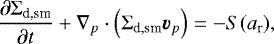
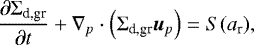
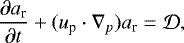
In our model, dust consists of two components: small (micron-sized) dust and grown dust. The former constitutes the initial reservoir for dust mass and is gradually converted in grown dust as the disk forms and evolves. Small dust is assumed to be coupled to gas, meaning that we only solve the continuity equation for small dust grains, while the dynamics of grown dust is controlled by friction with the gas component and by the total gravitational potential of the star, and the gaseous and dusty components. The conversion from small to grown dust is considered by calculating the dust growth rate S. The resulting continuity and momentum equations for small and grown dust are $\frac{\partial Σ_{d, sm}}{\partial t} + \nabla_{p} \cdot (Σ_{d, sm} v_{p}) = - S (a_{r}),$ $\begin{equation*}\frac{{\partial \Sigma_{\textrm{d,sm}} }}{{\partial t}} + \nabla_p \cdot \left( \Sigma_{\textrm{d,sm}} {\bm{v}}_p \right) = - S(a_{\textrm{r}}), \end{equation*}$ (5) $\frac{\partial Σ_{d, gr}}{\partial t} + \nabla_{p} \cdot (Σ_{d, gr} u_{p}) = S (a_{r}),$ $\begin{equation*}\frac{{\partial \Sigma_{\textrm{d,gr}} }}{{\partial t}} + \nabla_p \cdot \left( \Sigma_{\textrm{d,gr}} {\bm{u}}_p \right) = S(a_{\textrm{r}}), \end{equation*}$ (6) $\begin{array}{l} \frac{\partial}{\partial t} (Σ_{d, gr} u_{p}) + {[\nabla \cdot (Σ_{d, gr} u_{p} \otimes u_{p})]}_{p} \\ = Σ_{d, gr} g_{p} + Σ_{d, gr} f_{p} + S (a_{r}) v_{p}, \end{array}$ $\begin{eqnarray*}\hspace*{-6pt}&&\frac{\partial}{\partial t} \left( \Sigma_{\textrm{d,gr}} {\bm{u}}_p \right) + \left[\nabla \cdot \left( \Sigma_{\textrm{d,gr}} {\bm{u}}_p \otimes {\bm{u}}_p \right)\right]_p\nonumber\\ \hspace*{-6pt}&&\quad = \Sigma_{\textrm{d,gr}} \, {\bm{g}}_p +\, \Sigma_{\textrm{d,gr}} {\bm{f}}_p + S(a_{\textrm{r}}) {\bm{v}}_p, \end{eqnarray*}$ (7)

where Σ_d,sm and Σ_d,gr are the surface densities of small and grown dust, u_p describes the planar components of the grown dust velocity, S(a_r) is the rate of conversion from small to grown dust per unit surface area and a_r is the maximum radius of grown dust. In this study, we assume that dust and gas are vertically mixed, which is justified in young gravitationally unstable and/or MRI active disks (Rice et al. 2004; Yang et al. 2018). However, in more evolved disks dust settling becomes significant. Its effect on the global evolution of gaseous and dusty disks was considered in our previous study (Vorobyov et al. 2018), showing that dust settling accelerates somewhat the small-to-grown dust conversion.

Equations (2)–(4) and (5)–(7) are solved using the operator-split solution procedure consisting of the transport and source steps. In the transport step, the update of hydrodynamic quantities due to advection is done using the third-order piecewise parabolic interpolation scheme of Colella & Woodward (1984). In the source step, the update of hydrodynamic quantities due to gravity, viscosity, cooling, and heating, and also friction between gas and dust components is performed. This step also considers the transformation of small to grown dust and also the increase in dust radius a_r due to growth. The small-to-grown dust conversion is defined as 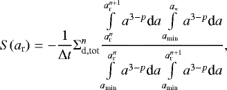$S (a_{r}) = - \frac{1}{\UpDelta t} Σ_{d, tot}^{n} \frac{\int_{a_{r}^{n}}^{a_{r}^{n + 1}} a^{3 - p} d a \int_{a_{min}}^{a_{*}} a^{3 - p} d a}{\int_{a_{min}}^{a_{r}^{n}} a^{3 - p} d a \int_{a_{min}}^{a_{r}^{n + 1}} a^{3 - p} d a},$ $\begin{equation*}S(a_{\textrm{r}}) = - {1 \over \UpDelta t } \Sigma_{\textrm{d,tot}}^n { \int \limits_{a_{\textrm{r}}^n} \limits^{a_{\textrm{r}}^{n+1}} a^{3-p} \textrm{d}a \int \limits_{a_{\textrm{min}}} \limits^{a_{\ast}} a^{3-p} \textrm{d}a \over \int \limits_{a_{\textrm{min}}} \limits^{a_{\textrm{r}}^n} a^{3-p} \textrm{d}a \int \limits_{a_{\textrm{min}}} \limits^{a_{\textrm{r}}^{n+1}} a^{3-p} \textrm{d}a }, \end{equation*}$ (8)

where Σ_d,tot = Σ_d,gr + Σ_d,sm is the total surface density of dust, indices $a_{r}^{n}$ $a_{\textrm{r}}^n$ and $a_{r}^{n + 1}$ $a_{\textrm{r}}^{n+1}$ the maximum dust radii at the current and next time steps, a_min = 0.005 μm the minimum radius of small dust grains, a_* = 1.0 μm a threshold value between small and grown dust components, and p = 3.5 the slope of dust distribution over radius. The evolution of the maximum radius a_r is described as $\frac{\partial a_{r}}{\partial t} + (u_{p} \cdot \nabla_{p}) a_{r} = D,$ $\begin{equation*} {\partial a_{\textrm{r}} \over \partial t} + (u_{\textrm{p}} \cdot \nabla_p ) a_{\textrm{r}} = \cal{D},\end{equation*}$ (9)

where the growth rate $D$ $\cal{D}$ accounts for the dust evolution due to coagulation and fragmentation. More details on the dust growth scheme can be found in Vorobyov et al. (2018).

We use the polar coordinates (r, ϕ) on a 2D numerical grid with 256 × 256 grid zones. The radial grid is logarithmically spaced, while the azimuthal grid is uniformly distributed. To avoid time steps that are too small, we introduce a central axisymmetric cell with a radius of 1.0 au (see detailed description below). The use of the logarithmically spaced grid in the r-direction and uniformly distributed grid in the ϕ-direction allowed us to resolve the disk in the vicinity of the central cell with a numerical resolution as small as 0.036 au.

3 Model of the central smart cell

In this section we describe the model adopted for the central cell. Since the model allows matter to flow in both directions through the interface between the central cell and the active disk, the term “sink cell” (often used in numerical simulations of protoplanetary disks) is no longer appropriate. In the following text, we use the term CSC to emphasize that the central cell has a subgrid physics, which we describe below.

Our model of the CSC calculates the total mass of gas and dust that is contained in the innermost unresolved disk region, taking in a simplified manner the MRI into account. The radius of this region is set to r_csc = 1.0 au. The balanceof mass in the CSC is computed using the following system of ordinary differential equations: 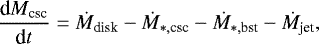$\frac{d M_{csc}}{d t} = {\dot{M}}_{disk} - {\dot{M}}_{*, csc} - {\dot{M}}_{*, bst} - {\dot{M}}_{jet},$ $\begin{equation*} {\textrm{d}M_{\textrm{csc}} \over{\textrm{d}t} }= \dot{M}_{\textrm{disk}}-\dot{M}_{*, \textrm{csc}}-\dot{M}_{*, \textrm{bst}}-\dot{M}_{\textrm{jet}},\end{equation*}$ (10) $\frac{d M_{*}}{d t} = {\dot{M}}_{*, csc} + {\dot{M}}_{*, bst} .$ $\begin{equation*}{\textrm{d}M_{*} \over{\textrm{d}t} } = \dot{M}_{*, \textrm{csc}}+\dot{M}_{*,\textrm{bst}} .\end{equation*}$ (11)

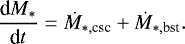
Here, Ṁ_disk is the mass accretion rate through the CSC–disk interface calculated in the hydrodynamics code as the mass flux passing through the inner disk boundary. We note that Ṁ_disk can be both positive (the matter flows from the disk to the CSC) and negative (the matter flows from the CSC to the disk), depending on the direction of velocity vector at the CSC–disk interface. The mass accretion rate from the CSC on the star is split into two parts: Ṁ_*,csc reflecting the regular mode of mass accretion from the CSC to the star and Ṁ_*,bst denoting the burst mode of accretion caused by the thermally ignited MRI in the CSC. The former is calculated as ${\dot{M}}_{*, csc} = {\begin{array}{l} ξ {\dot{M}}_{disk} & for $ {\dot{M}}_{disk} > $ 0, \\ 0 & for $ {\dot{M}}_{disk} ⩽ $ 0, \end{array}$ $\begin{equation*} \dot{M}_{*, \rm csc}= \begin{cases} \xi \dot{M}_{\textrm{disk}} &\text{for $\dot{M}_{\textrm{disk}} > $ 0},\\[3pt] 0 &\text{for $\dot{M}_{\textrm{disk}} \leqslant $ 0}, \end{cases} \end{equation*}$ (12)

where we assumed that mass accretion from the CSC on the star is a fraction ξ of mass accretion from the disk to the CSC. The limit of small ξ ≈ 0 corresponds to slow mass transport through the CSC, resulting in gradual mass accumulation in the sink. Slow mass transport may be caused by the development of a dead zone in the CSC. The opposite limit of large ξ ≈ 1.0 assumes fast mass transport, so that the matter that crosses the CSC–disk interface does not accumulate in the CSC, but is quickly delivered on the star. Physically, this means that mass transport mechanisms of similar efficiency operate in the disk and in the CSC.

The Ṁ_*,bst term in Eq. (10) accounts for accretion bursts, which may occur in the CSC through the thermal ignition of the MRI. The MRI burst activates when the gas temperature exceeds the thermal ionization threshold, usually assumed to be above 1000 K. Since we do not calculate the gas temperature in the CSC, we instead assume that the burst is activated when the gas surface density in the CSC exceeds 2 × 10⁴ g cm⁻², in accordance with the study of Bae et al. (2014). We check the gas temperature at the CSC–disk interface at the onset of the burst and confirm that the gas temperature exceeds 1000 K. When the MRI burst activates, the accretion rate is set equal to Ṁ_*,bst = 10⁻⁴ M_⊙ yr⁻¹. If the burst duration exceeds 70 yr or the gas surface density in the central cell drops below 100 g cm⁻², the burst terminates. The adopted parameters of the bursts can vary within a factor of several, but this is not expected to affect our simulations qualitatively.

The last term on the right-hand side of Eq. (10) is the mass ejection rate by the jets. It is defined as Ṁ_jet = η(Ṁ_*,csc + Ṁ_*,bst), where η is a portion of matter that is ejected by the jets. The actual value of η varies from 0.01 to 0.5. In this research we used a fixed value of η = 0.1 and leave a more detailed investigation of the effects of varying η for a furtherstudy. Finally, we note that Eqs. (10) and (11) should be applied separately to the gas and dust components. The system of Eqs. (10) and (11) is solved at each hydrodynamical time step to obtain the masses of gas and dust in the CSC. The graphical representation of the CSC model is given in Fig. 1.

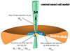Fig. 1

Graphical representation of the central smart cell (CSC) in the general context of the protostellar disk model. The main mass transport rates through the CSC are indicated with the arrows.

4 Boundary and initial conditions

The choice of boundary conditions in core collapse simulations always presents a certain challenge. While the outer boundary can be reflecting, meaning that no matter can cross the boundary, the inner boundary cannot be of that type. The code must allow matter to freely flow through the CSC–disk interface. If the inner boundary allows matter to flow only in one direction, i.e., from the disk to the CSC, then any wave-like motions near the inner computational boundary, such as those triggered by spiral density waves in the disk, would result in a disproportionate flow through the CSC–disk interface. As a consequence, an artificial depression in the gas density near the inner boundary develops in the course of time because of the lack of compensating back-flow from the CSC to the disk. This was the reason why Ṁ_disk in Eq. (10) can have both a positive and negative sign depending on the direction of gas and dust flow through the CSC–disk interface.

To proceed with numerical simulations, we need to define the values of surface densities, velocities, and gas internal energy at the computational boundaries. Let us first consider the inner computational boundary. The surface densities of gas and dust at the inner boundary can be directly obtained by solving Eqs. (10) and (11). We note that Eq. (10) returns the masses of gas and dust in the CSC, but these quantities can be turned into the corresponding surface densities when divided by the fixed area of the CSC. We do not have information on the internal energy or velocity in the CSC. Therefore, the radial velocity and internal energy at the inner boundary are determined from the zero gradient condition at the CSC–disk interface, while the azimuthal velocity is extrapolated from the active disk to the CSC assuming a Keplerian rotation. We note that these boundary conditions enable a smooth transition of the surface density between the inner active disk and the CSC, preventing (or greatly reducing) the formation of an artificial drop in the surface density near the inner boundary. A more detailed study of the effects of the inner boundary condition on the disk evolution is deferred to a separate study. We ensure that our boundary conditions conserve the total mass budget of gas and dust in the system. Finally, we note that the outer boundary condition (usually located at several thousands of au from the star) is set to a standard free outflow, allowing material to flow out of the computational domain, but not allowing any material to flow in. The zero-gradient condition is applied to all hydrodynamic quantities.

The initial radial profile of the gas surface density Σ_g and angular velocity Ω of the pre-stellar core has the form $Σ_{g} = \frac{r_{0} Σ_{g, 0}}{\sqrt{r^{2} + r_{0}^{2}}},$ $\begin{equation*} \Sigma_{\textrm{g}}\,{=}\,\frac{r_{0}\Sigma_{\textrm{g,0}}}{\sqrt{r^{2}+r_{0}^{2}}},\end{equation*}$ (13) $Ω = 2 Ω_{0} {(\frac{r_{0}}{r})}^{2} [\sqrt{1 + {(\frac{r}{r_{0}})}^{2}} - 1],$ $\begin{equation*} \UpOmega\,{=}\,2\Omega_{0}\left(\frac{r_{0}}{r}\right)^{2}\left[\sqrt{1+\left(\frac{r}{r_{0}}\right)^{2}}-1\right],\end{equation*}$ (14)

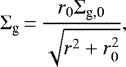
where Σ_g,0 and Ω₀ are the angular velocity and gas surface density at the center of the core and 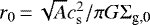$r_{0} = \sqrt{A} c_{s}^{2} / π G Σ_{g, 0}$ $r_{0}\,{=}\,\sqrt{A}c_{\mathrm{s}}^{2}/\pi G\Sigma_{\textrm{g,0}}$ is the radius of the central plateau, where c_s is the initialisothermal sound speed in the core. This radial profile is typical of pre-stellar cores formed as a result of the slow expulsion of magnetic field due to ambipolar diffusion, with the angular momentum remaining constant during axially symmetric core compression (Basu 1997). The value of the positive density perturbation A is set to 1.1, making the core unstable to collapse. The initial gas temperature in collapsing cores is T_init = 20 K. We consider a numerical model with Ω₀ = 2.05 km s⁻¹ pc⁻¹, Σ_g,0 = 0.2 g cm^-2, and r₀ = 1200 AU. The resulting core mass M_core = 1.03 M_⊙ and the ratio of rotational to gravitational energy β_rot = 2.4 × 10⁻³. The initial dust-to-gas ratio is 1:100. All dust is initially in the form of small dust particles with a radius of 1.0 μm.

5 Results

In this work,we consider three values of the ξ-parameter controlling the rate of mass transport through the CSC. More specifically, ξ = 0.05 corresponds to slow mass transport through the CSC when only 5% of the mass that passes through the cell–disk interface (per unit time) arrives at the star and the remaining 95% is retained in the CSC. The choice of ξ = 0.95 corresponds to the fast transport regime when 95% of the mass accretes at the star and only 5% is retained in the CSC, ξ = 0.5 corresponds to the intermediate case.

In our model, the mass transport rate in the disk is controlled by viscous and gravitational torques. While gravitational torques operate self-consistently in our numerical simulations thanks to computed disk self-gravity, viscous torques are parameterized using the α-prescription of Shakura & Sunyaev (1973). The viscous α-parameter in the disk is set equal to 0.01, which is characteristic of a fully operational MRI (e.g., Yang et al. 2018). Lower values of the α-parameter will be considered in a follow-up study. The starting point of each simulation is the gravitational collapse of a pre-stellar core. In the adopted thin-disk approximation, the core has the form of a flattened pseudo-disk, a spatial configuration that can be expected in the presence of rotation and large-scale magnetic fields (e.g., Basu 1997). The initial ratio of rotational to gravitational energy is only β_rot = 2.4 × 10⁻³ and the core is initially unstable to gravitational collapse. As the collapse proceeds, the inner regions of the core spin up and a centrifugally balanced circumstellar disk forms at t = 55 kyr when the inner infalling layers of the core hit the centrifugal barrier near the CSC. The material that has passed to the CSC before the instance of circumstellar disk formation constitutes a seed for the central star, which grows further through accretion from the circumstellar disk. The infalling core continues to land at the outer edge of the circumstellar disk until the core depletes. The infall rates on the circumstellar disk are in agreement with what can be expected from the free-fall collapse (Vorobyov 2010). Computations continue up to 1.0 Myr, thus covering the entire embedded phase and the early T Tauri phase of disk evolution.

5.1 Global evolution of gas and dust in the disk

In this section we study the formation and long-term evolution of the circumstellar disk. The top row of Fig. 2 presents the temporal evolution of the azimuthally averaged gas surface density for models with three values of the ξ-parameter: 5% (left column), 50% (middle column), and 95% (right column). Circumstellar disks in the models with lower ξ are systematically denser than the models with higher ξ, particularly in the inner regions within r ≲ 30 au. In the ξ = 5% model, the mass transport rate through the CSC onto the star is only 5% that of the mass transport rate through the sink–disk interface. As a result the matter accumulates in the inner disk until the gas temperature reaches a critical threshold for the thermal ionization and an MRI-triggered accretion bursts sets in. The burst evacuates a larger fraction of the matter accumulated in the CSC and the process repeats itself. In contrast, in the ξ = 95% model the mass transport rate through the CSC and the mass transport rate at the CSC–disk interface are similar. As a consequence, the matter does not accumulate in the inner disk and the gas surface density is lower in the ξ = 95% model, as is evident from the isocontours outlining the disk regions with Σ_g ≥ 10³ g cm⁻². We also note that the ξ = 95% model never experiences MRI-triggered accretion bursts because the gas density and temperature never reach the thermal ionization threshold. The behavior of small dust particles is similar to that of the gas and is therefore not shown.

The temporal evolution of grown dust for each model is shown in the second row of Fig. 2. The black lines are isocontours with Σ_d,gr = 10 g cm⁻². The distribution of grown dust is slightly more extended and the surface density of grown dust is slightly higher in the ξ = 5% model, but the difference in the spatial distribution of grown dust is not as profound as in the case of gas. The similarity between the grown dust distributions is a direct consequence of efficient inward drift of grown dust. The lack of local gas pressure maxima in the disk, as the third row in Fig. 2 shows, allows grown dust to freely drift through the disk towards the CSC. This also explains a more compact spatial distribution of grown dust compared to that of gas.

The fourth row of Fig. 2 presents the azimuthally averaged gas temperature in the disk as a function of time. We note that the dust temperature is similar to that of gas in our model. The inner disk regions in models with lower ξ are warmer than in models with higher ξ because of higher surface densities and optical depths. We also note that the gas temperature in the ξ = 5% model can episodically exceed 1200–1300 K in the inner several au, triggering accretion bursts as described above (see also Fig. 6 in Sect. 5.2). We note that at these high temperatures dust may sublimate, an effect not taken into account in the current model.

The temporal evolution of the maximum dust grain radius a_r is presented in the fifth row of Fig. 2. Dust grains quickly grow from micron-sized particles to centimeter-sized pebbles in the inner disk area, several tens of au in width, during just several tens of thousands of years after the disk formation instance (which is marked by the horizontal dashed lines). Interestingly, in models with ξ = 50% and ξ = 95% the largest dust grains are concentrated in a ring at a distance of several tens of au from the star, rather than in the inner disk regions as in the ξ = 5% model. The reason for this distinct behavior is discussed in more detail later in the this section.

Finally, the bottom row of Fig. 2 presents the spatial distribution of the total dust-to-gas ratio ζ_d2g versus time. Significant deviations of ζ_d2g = (Σ_d,gr + Σ_d,sm) ∕ Σ_g from the canonical 1:100 value are notable in the inner disk regions. The most striking case is the ξ = 5% model, which demonstrates a decrease in ζ_d2g by almost an order of magnitude (compared to 1:100) in the inner region of the disk. Conversely, the other two models show an increase in ζ_d2g by factors of 2–3 near the CSC–disk interface.

To understand the reason for the decrease in ζ_d2g in the ξ = 5% model, we refer to the first and second rows of Fig. 2 showing the surface densities of gas and grown dust, respectively. Consider first the gas density distribution. Clearly, the ξ = 5% model is characterized by notably higher Σ_g than the other two models. This difference is caused by slow mass transport through the CSC. The resulting bottleneck leads to the accumulation of large amounts of gas in the disk inner regions. Furthermore, strong negative pressure gradients that develop in the inner disk (see the third row) prevent gas from freely flowing towards the star. Consider now the surface densities of grown dust, which spatial distributions are remarkably similar in models with different ξ. It is known that grown dust drifts in the direction of increasing gas pressure. Although small local pressure maxima may be present in the disk in the form of spiral arms, the general trend is evident: the gas pressure increases inward. As a result, dust freely drifts to the CSC in all three models and small differences in the drift speed may only arise due to variations in the Stokes number. The net effect is that the decrease in ζ_d2g that we witness in the ξ = 5% model is not due to dust depletion, but is due to gas accumulation in the inner disk. The opposite effect is seen in the ξ = 50% model and especially in the ξ = 95% model; a fast mass transport through the CSC leads to gas depletion in the inner 1 au near the CSC–disk interface. As a result, ζ_d2g increases there.

We further analyze the radial distribution of the maximum grain radius a_r in the disk. The blue lines in Fig. 3 present a_r versus radial distance in models with ξ = 95% (top panel) and ξ = 5% (bottom panel). The orange lines show the fragmentation barrier defined as 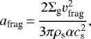$a_{frag} = \frac{2 Σ_{g} v_{frag}^{2}}{3 π ρ_{s} α c_{s}^{2}},$ $\begin{equation*} a_{\textrm{frag}}\,{=}\,\frac{2\Sigma_{\textrm{g}}v_{\textrm{frag}}^2}{3\pi\rho_{\textrm{s}}\alpha c_{\textrm{s}}^2},\end{equation*}$ (15)

where v_frag is a threshold value for the fragmentation velocity taken to be 30 m s⁻¹ in this study and ρ_s = 2.24 g cm⁻³ the materialdensity of grains. By definition, dust cannot grow in our model beyond the size defined by the fragmentation barrier. Thebouncing effects are not considered in our dust growth model. All radial profiles are plotted at t = 500 kyr.

Two interesting features can be seen in Fig. 3. First, the dust size is limited by the fragmentation barrier only in the inner 20–30 au. In the outer disk regions, the size of dust grains never reaches the fragmentation barrier. This means that the dust growth can be split into two systems: the fragmentation-limited regime in the inner disk and the drift-limited regime in the outer disk (e.g., Birnstiel et al. 2016). Second, the fragmentation barrier in the ξ = 95% model has a well-defined peak at 20 au and decreases towards the star, while in the ξ = 5% model the fragmentation barrier has a plateau in the inner 20–30 au. This explains the peculiar spatial distribution of dust sizes in the fifth row of Fig. 2; the maximum in a_r in the ξ = 95% model is reached at several tens of au and not in the innermost disk regions, as might be naively expected.

It is interesting to see how the total dust-to-gas ratio in the CSC evolves with time. Figure 4 presents the ζ_d2g values in the CSC as a function of time for the ξ = 95% model and ξ = 5% model. In the former, ζ_d2g stays at around 0.01 with small deviations from this canonical value. In the latter, however, ζ_d2g shows large deviations from the canonical value mainly to higher values. In the ξ = 5% model we therefore see an interesting trend: the total dust-to-gas ratio is decreased in the disk region between oneand ten au (see the bottom row in Fig. 2), but is enhanced in the CSC (i.e., at ≤1.0 au). We note that ζ_d2g may becomeeven higher in the innermost parts of the CSC if additional drift of grown dust takes place there. This, however, cannot be resolved in our numerical model.

Finally, the models with different rates of mass transport through the CSC are also characterized by distinct disk and stellar masses. In Fig. 5 we present the integrated masses of gas and grown dust in the disk and also the stellar mass as a function of time for the ξ = 5% model (blue lines) and ξ = 95% model (orange lines). Clearly, the ξ = 95% model has a systematically higher stellar mass, but lower gas disk mass than its ξ = 5% counterpart.Higher stellar masses and lower disk masses make gravitational instability less efficient (see Sect. 5.3 and Fig. 8). The mass of grown dust in the disk, however, differs only by a factor of unity between themodels, which is a consequence of fast and unhindered inward radial drift of grown dust in both models. We also note that the total mass of grown dust in the two models hardly reaches several tens of Earth masses beyond 1.0 au, a rather low value for efficient planet formation to set in, a feature also noted by Vorobyov et al. (2018).

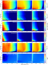Fig. 2

Temporal evolution of the azimuthally averaged gas surface density (top row), grown dust surface density (second row), gas pressure (third row), gas temperature (fourth row), maximum radius ofgrown dust (fifth row), and the dust-to-gas mass ratio (bottom row) in models with ξ = 5% (left column), ξ = 50% (middle column), and ξ = 95% (right column). Contour lines indicate gas surface densities of 10³ g cm⁻² (top row), grown dust surface densities of 10 g cm⁻² (second row), and gas temperatures of 1000 K to emphasize evolutionary trends. The horizontal dotted lines in the fifth row indicatethe disk formation instance.

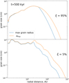Fig. 3

Radial profiles of the azimuthally averaged maximum radius of dust grains and fragmentation limit shown with the blue and orange lines, respectively. Top panel: model with ξ = 95%. Bottom panel: model with ξ = 5%.

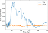Fig. 4

Evolution of the dust-to-gas mass ratio in the CSC. The blue and orange lines correspond to the ξ = 5% and ξ = 95% models, respectively.

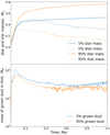Fig. 5

Total gas plus dust mass in the disk and stellar mass (top panel) and the mass of grown dust in the disk (bottom panel) in models with ξ = 5% (blue lines) and ξ = 95% (orange lines).

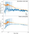Fig. 6

Accretion rate (top panel) and total stellar luminosity (bottom panel) for the ξ = 5% model (blue lines) and ξ = 95% model (orange lines).

5.2 Protostellar accretion

Mass accretion on the nascent protostar plays an important role in the dynamical and chemical evolution of a young stellar object. Accretion brings matter, angular momentum, and energy to the star, thus affecting its internal structure. Accretion also feeds back to the disk via accretion luminosity, providing the main source of disk heating in its intermediate and outer regions (including the envelope in the embedded phase). Determining the character of protostellar accretion is therefore one of the major problems in the theory of star formation.

Figure 6 shows the mass accretion rates on the star Ṁ_* = Ṁ_*,csc + Ṁ_*,bst and the total stellar luminosity L_tot (accretion and photospheric) in models with ξ = 5% and ξ = 95%. Clearly, Ṁ_* in the ξ = 5% model is highly variable in the early 0.15 Myr of evolution and shows frequent accretion bursts alternating with longer periods of quiescent low-rate accretion. At the same time, the ξ = 95% model is characterized by a gradually declining accretion rate with only low-amplitude flickering. Moreover, Ṁ_* in the ξ = 95% model is notably higher than the quiescent accretion rate in the ξ = 5% model (the latter stays around 10⁻⁷ M_⊙ yr⁻¹). A similar trend stands for the total stellar luminosity L_tot in the ξ = 5% model features strong outbursts, while the ξ = 95% model only shows low-amplitude variations. The latter model, nevertheless, is characterized by a higher L_tot in the quiescent mode.

This difference in the character of mass accretion and stellar radiative output may have important consequences for the stellar and disk evolution. Accretion bursts affect the physical characteristics and chemical composition of young protostars, causing peculiar excursions on the Hertzsprung–Russell diagram and changing their lithium abundance (Elbakyan et al. 2019; Baraffe et al. 2017). In addition, luminosity bursts raise the temperature of the disk, thus affecting its dynamics and chemical composition (Stamatellos et al. 2011; Molyarova et al. 2018). Finally, we note the accretion bursts in the ξ = 5% model; although they are quite intense and numerous, they do not make up for the quiescent accretion, and the final stellar mass in this model is notably lower than that of the ξ = 95% model without the bursts.

Figure 7 presents the gas temperature distribution in the 600 × 600 au² box in models with ξ = 5% (top panels) and ξ = 95% (bottom panels). Three time instances are chosen to show the temperature distribution in the ξ = 5% model before the burst (t = 157 kyr), during the burst (t = 158 kyr), and after the burst (t = 159 kyr). The ξ = 95% model has no bursts, but its temperature distribution is shown at the same times for comparison. We note that the isolated blobs of hot gas that are seen in the upper panels are gaseous clumps formed via disk gravitational fragmentation. Clearly, during the burst the gas temperature exceeds the pre- and post-burst values by a factor of several. Furthermore, the insets in the right column demonstrate that the disk is warmer in the ξ = 95% model and is colder in the ξ = 5% model during the quiescent phase of accretion. This difference in gas temperatures has an important consequence for the longevity of disk gravitational instability, as we will see later in Sect. 5.3. We conclude that the rate of mass transfer through the CSC has a significant effect on the character of mass accretion and luminosity of the nascent protostar.

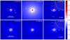Fig. 7

Top row: spatial maps of the gas temperature in the inner 600 × 600 au² box before an accretion burst (left panel), during the burst (middle panel), and after the burst (right panel) for the ξ = 5% model. Bottom row: spatial maps of the gas temperature in the ξ = 95% model characterized by steady accretion without bursts. The same evolutionary times as for the ξ = 5% model are shown. The inset plots in the right column present the azimuthally averaged temperature on the same spatial scale as the 2D temperature maps. The scale bar is in log Kelvin.

5.3 Gravitational instability and fragmentation

Gravitational instability and fragmentation are among the most important physical phenomena that occur in the early evolution of protostellar disks. Gravitational instability is a major mass and angular momentum transport mechanism in the embedded phase of disk evolution (Vorobyov & Basu 2009), while gravitational fragmentation is thought to be a likely gateway for the formation ofgiant planets and brown dwarfs (Boss 2003; Mayer et al. 2007; Stamatellos & Whitworth 2009; Forgan & Rice 2011; Vorobyov 2013, 2016; Meru 2015; Nayakshin 2017). In addition, disk fragmentation can trigger accretion bursts caused by inward migration and infall of gaseous clumps on the star (e.g., Vorobyov & Basu 2005, 2015; Machida et al. 2014; Meyer et al. 2017; Zhao et al. 2018; Vorobyov & Elbakyan 2018). Gravitational instability and fragmentation occurs in the intermediate and outer disk regions and it appears at first glance that physical processes in the CSC are unlikely to influence this phenomenon. However, as we saw in Figs. 2 and 5, the rate of masstransport through the CSC can affect the disk mass, gas density, and temperature distributions in the bulk of the disk, which in turn can have implications for the development of gravitational instability and fragmentation.

Figure 8 presents the gas surface density distributions in the inner 250 × 250 au² box in all three considered models with distinct ξ-parameters at consecutive evolutionary times as indicated in the first column. More specifically, the first, second, and third columns present the models with ξ = 5%, ξ = 50%, and ξ = 95%, respectively.The early evolution in all models is qualitatively similar and the disk is characterized by strong gravitational instability. Fragmentation is also evident in several panels. However, the subsequent evolution demonstrates notable differences. For instance, the ξ = 95% model has a nearly axisymmetric disk already at 400 kyr, while the other models have a well-defined spiral structure at this evolutionary time. This difference in the longevity of gravitational instability can in part be explained by the apparent difference in the disk and stellar masses in these models. As Fig. 5 shows, the disk mass is the lowest and the stellar mass is the highest in the ξ = 95% model, both acting to stabilize the disk against gravitational instability. In addition, a systematically higher gas temperature of the disk in the ξ = 95% model works for faster disk stabilization.

The strength of gravitational instability can be quantified using the Fourier amplitudes defined as 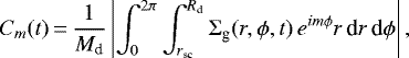$C_{m} (t) = \frac{1}{M_{d}} | \int_{0}^{2 π} \int_{r_{sc}}^{R_{d}} Σ_{g} (r, ϕ, t) e^{i m ϕ} r d r d ϕ |,$ $\begin{equation*} C_{m} (t) \,{=}\, {1 \over M_{\textrm{d}}} \left| \int_0^{2 \pi} \int_{r_{\textrm{sc}}}^{R_{\textrm{d}}} \Sigma_{\textrm{g}}(r,\phi,t) \, e^{im\phi} r \, \textrm{d}r\, \textrm{d}\phi \right|,\end{equation*}$ (16)

where M_d is the disk mass, R_d is the disk’s physical outer radius, and m is the azimuthal wave number of the disk’s spiral mode. When the disk surface density is axisymmetric, the amplitudes of all modes are equal to zero. When, for example, C_m(t) = 0.1, the perturbation amplitude of spiral density waves in the disk is 10% that of the underlying axisymmetric density distribution.

Figure 9 presents the global Fourier amplitudes as a function of time for the m = 1, m = 2, and m = 3 spiral modes. The solid and dashed lines correspond to the ξ = 5% and ξ = 95% models, respectively. The models are both characterized by C_m that are highest in the early evolution but decrease with time, reflecting a gradual decline in the strength of gravitational instability. The decline is, however, the fastest in the ξ = 95% model, in agreement with the fastest stabilization of the disk discussed in the context of Fig. 8. We also note an interesting feature seen in the ξ = 5% model where episodic surges in C_m are apparent between 0.3 and 0.7 Myr. The nature of these events is discussed in more detail below.

We have already pointed out that our models exhibit not only gravitational instability, but also gravitational fragmentation. In Fig. 10 we plot the total number of fragments that simultaneously exist in the disk for the ξ = 5% (top panel), ξ = 50% model (middle panel), and ξ = 95% models (bottom panel). We distinguish the newly formed fragments using the fragment-tracking method described in detail in Vorobyov & Elbakyan (2018). This method requires that the fragment is pressure-supported, having a negative pressure gradient with respectto the center of the fragment, and also that the fragment is kept together by gravity, with the potential well being deepest at the center of the fragment. We first scan the disk for the local density enhancements above a certain density limit. If anyof the two conditions fails at the center of the density enhancement, then this candidate is rejected, meaning that we falsely took a local density perturbation for a pressure-supported, gravity-bound fragment. If both conditions are fulfilled at the center of the density enhancement, we continue outward from the center and check the neighbouring cells until any of the two conditions is violated. The grid cells that fulfill both conditions constitute the fragment.

Let us first consider the ξ = 5% model. The first fragment forms as soon as 80 kyr after the onset of the simulation (or 25 kyr after disk formation) and is followed by an uninterrupted series of fragmentation events lasting ≈ 150 kyr, during which time fragments are constantly present in the disk. The maximum number of fragments existing simultaneously in the disk is eight. In the following evolution, the disk enters an episodic fragmentation mode with major fragmentation episodes occurring at 270, 300, 410, and 530 kyr. In contrast, disk fragmentation in the ξ = 50% and ξ = 95% models is less pronounced. It starts later, ends sooner, and forms fewer fragments at a time than in the ξ = 5% model. The episodic fragmentation mode is suppressed; fragmentation ends after 270 kyr and no fragments are found in the later evolution. This difference in the intensity of disk fragmentation is concordant with the corresponding difference in the strength of gravitational instability (see Fig. 8) and is caused by distinct disk masses, stellar masses, and disk temperatures in these three models, as was discussed above.

Interestingly, the episodic fragmentation events take place in the Class II phase of disk evolution, the onset of which is shown by the dashed vertical line in Fig. 10, and is defined as the time instance when less than 5% of the initial mass reservoir of the pre-stellar core is left in the infalling envelope. It is usually thought that disk fragmentation is most likely to develop in the embedded phase of disk evolution when mass-loading from the envelope replenishes the disk mass loss via accretion and sustains the disk in the unstable mode (e.g., Vorobyov & Basu 2005; Kratter et al. 2008). Our numerical simulations indicate that disk fragmentation is also possible in more evolved disks when mass-loading is no longer operational. We define the evolutionary state when at least one fragment exists in the disk as the “fragmented-disk state”. Conversely, the “stable-disk state” denotes the state when no fragments are found in the disk. We note that the lifetime of the fragments may be underestimated because of limited numerical resolution, which may cause their premature destruction via tidal torques. Thus, the duration of the fragmented-disk state is to be considered a lower limit.

The fragmented-disk and stable-disk states are highlighted in Fig. 10. Clearly, the time spent in the stable-disk state is longer than in the fragmented-disk state. When considering only the early T Tauri phase (200–700 kyr), the ξ = 5% model spends 80% of its lifetime in the stable-disk state and only 20% in the fragmented-disk state. This means that detecting a Class II disk in the stable-disk state is more likely than in the fragmented-disk state, especially considering that disk fragmentation ends after about 0.5 Myr of disk evolution.

A useful quantity that describes the disk propensity to gravitational instability and fragmentation is the Toomre Q-parameter. For a mixture of gas and dust the Q-parameter can be defined as 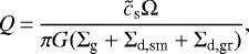$Q = \frac{{\tilde{c}}_{s} Ω}{π G (Σ_{g} + Σ_{d, sm} + Σ_{d, gr})},$ $\begin{equation*} Q\,{=}\,{\tilde{c}_{\textrm{s}} \UpOmega \over \pi G (\Sigma_{\textrm{g}}+\Sigma_{\textrm{d,sm}} + \Sigma_{\textrm{d,gr}})},\end{equation*}$ (17)

where ${\tilde{c}}_{s} = c_{s} / \sqrt{1 + ζ_{d2g}}$ $\tilde{c}_{\textrm{s}}\,{=}\,c_{\textrm{s}}/\sqrt{1+\zeta_{\textrm{d2g}}}$ the modified sound speed in the presence of dust. As follows from its definition, the Toomre parameter depends on the local characteristics in the disk and can vary throughout the disk extent. To relate the fragmented-disk state with the Q-parameter, we need to choose a representative Q-value for the entire disk. Since the disk propensity to gravitational instability is inversely proportional to the Q-value, we search for the minimum values of Q at every radial annulus in the disk and then arithmetically average the resulting minimum values to derive the mean minimum Toomre parameter ${\bar{Q}}_{min}$ $\overline Q_{\textrm{min}}$ for the disk.We exclude the inner 15 au of the disk from this procedure since this region is characterized by Q-values that are much higher than 2.0 due to high temperature and strong shear. The resulting quantity is plotted in Fig. 10. In the fragmented-disk state the ${\bar{Q}}_{min}$ $\overline Q_{\textrm{min}}$ -values drop often below 1.0, while in the stable-disk mode they rise above 2.0, which is consistent with the theoretical expectations.

To further investigate the episodic mode of disk fragmentation, we plot in Fig. 11 the gas surface density distributions in the ξ = 95% model (top row) and ξ = 5% model (bottom row) during an evolutionary period of 105 kyr starting from t = 530 kyr after the onset of pre-stellar core collapse. At this evolutionary stage, the disk is about 480 kyr old and is in the T Tauri stage of evolution, where gravitational fragmentation is not expected to be a dominant mode of evolution. Indeed, in the ξ = 95% model the disk is smooth, axisymmetric, and gravitationally stable. At the same time, the disk in the ξ = 5% model experiences a transitory episode of vigorous gravitational instability and fragmentation. The black contour lines delineate disk regions where the Toomre Q-parameter is smaller than unity. Clearly, the Q-parameter drops below unity only in the ξ = 5% model showing disk fragmentation, in agreement with the theoretical predictions.

The diagrams in Fig. 12 presents the normalized number of fragments as a function of their mass in the ξ = 5% model (top panel), ξ = 50% model (middle panel), and ξ = 95% model (bottom panel). We searched for the presence of fragments in the disk every 1.0 kyr of disk evolution, for a total of almost 1000 time snapshots. We then used these snapshots to calculate the total number of fragments that were present in the disk during its entire evolution. Since the lifetime of a fragment in the disk may be longer than 1.0 kyr, this procedure implies that some fragments may have been counted several times, and is the reason why we provided the normalized number of fragments and not their absolute number. This procedure also means that our diagrams favor fragments with the longest lifetimes, which, in our opinion, is sensible. Clearly, the peak of the mass distribution is at 4–6 M_Jup and the number of fragments drops quickly on both sides of the peak. The lowest mass is 2 M_Jup and the highest is 30 M_Jup. If we set an upper mass limit of 13 M_Jup for a giant planet, then most fragments are in the planetary mass regime.

The numerical resolution of our simulations does not allow us to reliably follow the fate of the fragments while they are destroyed by tidal torques. However, higher resolution simulations have demonstrated that fragments may survive and form massive giant planets and brown dwarfs on wide orbits (e.g., Vorobyov & Elbakyan 2018). It remains to be seen what consequences the delayed formation of giant planets and/or brown dwarfs may have on the structuring of planetary systems. We conclude that disk fragmentation is a likely phenomenon in the evolution of massive circumstellar disks, but its intensity and longevity depend sensitively on the value of ξ. We plan to address the episodic fragmentation mode in more detail in follow-up higher resolution studies.

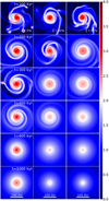Fig. 8

Gas surface density maps in the inner 250 × 250 au² box shown at consecutive evolutionary times for all three models with distinct ξ-parameters. Time is indicated in the left column and is counted from the onset of numerical simulations and the disk forms at 56 kyr. The scale bar is in log g cm⁻².

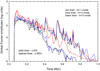Fig. 9

Global Fourier amplitudes. The solid and dashed lines correspond to models with slow (ξ = 5%) and fast (ξ = 95%) mass transport through the CSC, respectively. Shown are the Fourier amplitudes for the first three modes: m = 1, m = 2, and m = 3 in red, blue,and black, respectively.

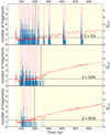Fig. 10

Total number of fragments present in the entire disk as a function of time in the ξ = 5% model (top panel), ξ = 50% model (middle panel), and ξ = 95% model (bottom panel). The vertical dashed lines indicate the onset of the Class II phase of disk evolution. Pink zones correspond to time periods in the Class II phase when fragments exist in the disk, and yellow zones show the time periods without any fragments in the disk. The red lines show ${\bar{Q}}_{min}$ $\overline Q_{\textrm{min}}$ , the mean minimum Toomre parameter in the disk.

Fig. 11

Gas surface density maps in the inner 600 × 600 au² box shown during a short time period between 530 kyr and 635 kyr for the ξ = 95% model (top panels) and ξ = 5% model (bottom panels). The black contour lines outline the disk regions where the Toomre Q-parameter is smaller than unity. The time is counted from the onset of numerical simulations. The disk is formed at 56 kyr. The scale bar is in log g cm⁻².

5.4 Orbital diversity of exoplanets

The known exoplanets have a surprising diversity of characteristics, such as mass, density, and atmospheric composition. In particular, the orbital positions of exoplanets range from ≲0.1 au to several hundreds of au. In this section we compare our model predictions with the orbital distribution of known exoplanets.

The color map in Fig. 13 shows the azimuthally averaged distribution of grown dust versus time. We took an arithmetic averaging of Σ_d,gr in models with three different values of ξ. The surface density of grown dust in the CSC is calculated as a ratio of the known mass of grown dust in the CSC (see Eq. (10)) to the surface area of the CSC. The outer boundary of the CSC is 1.0 au and the inner boundary of the CSC is set equal to the dust sublimation radius $r_{csc}^{in}$ $r^{\textrm{in}}_{\textrm{csc}}$ , which is calculated as 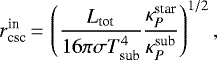$r_{csc}^{in} = {(\frac{L_{tot}}{16 π σ T_{sub}^{4}} \frac{κ_{P}^{star}}{κ_{P}^{sub}})}^{1 / 2},$ $\begin{equation*} r^{\textrm{in}}_{\textrm{csc}} \,{=}\, \left(\frac {L_{\textrm{tot}}}{16 \pi \sigma T_{\textrm{sub}}^4} \frac{\kappa_{P}^{\textrm{star}}}{\kappa_{P}^{\textrm{sub}}}\right)^{1/2},\end{equation*}$ (18)

where L_tot is the total stellar luminosity provided by our models; σ is the Stefan–Boltzmann constant; T_sub is the dust sublimation temperature assumed to be equal to 1500 K; $κ_{P}^{star}$ $\kappa_{P}^{\textrm{star}}$ is the Planck mean opacity calculated for the effective temperature of the central star, which in turn is determined from the stellar evolution tracks; and $κ_{P}^{sub}$ $\kappa_{P}^{\textrm{sub}}$ is the Planck mean opacity calculated for the dust sublimation temperature. We note that $κ_{P}^{sub}$ $\kappa_{P}^{\textrm{sub}}$ is constant, but $κ_{P}^{star}$ $\kappa_{P}^{\textrm{star}}$ changes with time as the central star evolves. We also note that Eq. (18) does not consider that dust grains can be back-heated by dust at larger radii, in which case $r_{csc}^{in}$ $r^{\textrm{in}}_{\textrm{csc}}$ may increase by a factor of order unity. Two vertical dotted lines in Fig. 13 highlight the disk regions within which the formation of giant planets via disk gravitational fragmentation is feasible (e.g., Vorobyov 2013; Stamatellos 2015; Vorobyov & Elbakyan 2018). The orbital positions of exoplanets as a function of their mass are indicated with the blue circles. We note that a jump in the dust surface density at r ≤ 1.0 au is caused by inward drift and accumulation of grown dust in the CSC.

Let us first consider the outer parts of the disk. Figures 8 and 11 demonstrate that gravitational instability and fragmentation are operational at distances from tens to hundreds of au. Because of insufficient numerical resolution of our models, the forming fragments are destroyed by tidal torques when migrating towards the star. However, higher resolution simulations indicate that a small fraction of the fragments may survive, open a gap, and settle on orbits from tens of au to hundreds of au, thus giving birth to giant planets on wide orbits (e.g., Vorobyov 2013; Stamatellos 2015; Vorobyov & Elbakyan 2018). The range of planetary orbits that may be accounted for by disk gravitational fragmentation is shown by two dashed vertical lines in Fig. 13. Moreover, the role of gravitational fragmentation may not be limited to the formation of giant planets on wide orbits. Tidal downsizing of gaseous envelopes of giant planets may turn them into icy giants and even into super-Earths, and these lighter planetary embryos may continue migrating towards the star, creating a population of close-orbit planets (see review by Nayakshin 2017).

Let us now consider the innermost parts of the disk where the highest accumulation of grown dust is found. In our models, dust does not grow beyond the fragmentation barrier a_frag (see Eq. (15)), effectively limiting the dust size to centimeters or decimeters at most. However, a streaming instability is thought to be a mechanism that helps overcome the fragmentation barrier, thus assisting the formation of planetesimals and planetary cores in protoplanetary disks (e.g., Johansen et al. 2007). We do not model the gas dynamics in the CSC, but it is possible to check whether conditions for the development of a streaming instability are satisfied in the CSC. For these conditions, we choose those suggested by the study of Yang et al. (2017). The black solid line in Fig. 14 divides the ζ_d2g–St phase space into the region prone to streaming instability (in green) and the region where streaming instability is suppressed (in brown). Here, ζ_d2g is the ratio of total dust to gas surface densities and St is the Stokes number defined as 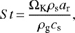$S t = \frac{Ω_{K} ρ_{s} a_{r}}{ρ_{g} c_{s}},$ $\begin{equation*} { St}\,{=}\,\frac{\Omega_{\textrm{K}}\rho_{\textrm{s}} a_{\textrm{r}}}{\rho_{\textrm{g}}c_{\textrm{s}}},\end{equation*}$ (19)

where ρ_g is the gas volume density calculated as ρ_g = Σ_g ∕ $(\sqrt{2 π} H_{g})$ $(\sqrt{2\pi} {H_{\textrm{g}}})$ , ρ_s = 2.24 g cm⁻³ the material density of grains, and Ω_K is the Keplerian velocity. The maximum radius of dust grains a_r in the CSC is assumed to be equal to the fragmentation radius a_frag, which is a legitimate assumption for the inner fragmentation-limited disk regions (see Fig. 3). For the speed of sound c_s we take the corresponding values at the CSC–disk interface. We note that ζ_d2g can be directly derived from our model of the CSC (see Sect. 3).

The blue circles in Fig. 14 present ζ_d2g versus St calculated for the CSC in the ξ = 5% model. Clearly, a streaming instability can develop in this model and the percentage of time that this model spends in the unstable regime is substantial, 45.5% compared to 54.5% in the stable regime. Even if we admit an order of magnitude uncertainty in calculating the Stokes number, a streaming instability can still develop in the CSC. At the same time, the cyan circles calculated for the ξ = 95% model demonstrate that a streaming instability cannot develop in this model. Finally, we note that the region of streaming instability in Fig. 14 is derived assuming an efficient dust settling to the disk midplane, with the dust vertical scale height H_d,gr being equal to or smaller than 2% that of the gas. The ratio H_d,gr ∕ H_g can be inferred from Dubrulle et al. (1995) as 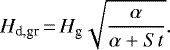$H_{d, gr} = H_{g} \sqrt{\frac{α}{α + S t}} .$ $\begin{equation*} H_{\textrm{d,gr}}\,{=}\,H_{\textrm{g}} \sqrt{{\alpha \over \alpha+St}}.\end{equation*}$ (20)

For the typical values of St ~ 0.1, the required ratio of H_d,gr ∕ H_g≲0.02 implies α≲10⁻⁴. Such low values of the α-parameter can be achieved if the MRI is mostly suppressed in the CSC, which is consistent with an assumed low mass transport rate through the CSC in the ξ = 5% model. We admit that more accurate numerical simulations extending in the inner sub-au region of the disk are needed to make firmer conclusions. If a streaming instability is indeed operational, this would lead to the formation of solid planetary embryos at orbital positions of ≲1.0 au. These protoplanets may later be scattered to larger orbital distances (e.g., Marleau et al. 2019) or migrated to smaller distances, gaining in the process gaseous atmospheres according to the core accretion scenario. Disk hydrodynamics simulations coupled to a planetary population synthesis model are needed to further explore this scenario.

We therefore foresee two planet-forming mechanisms that may operate concurrently in the disk: a streaming instability in the innermost parts of the disk (working concurrently with the core accretion scenario if solid protoplanetary cores exceed a critical mass) and gravitational fragmentation in the outermost parts of the disk. In the future, we plan to couple our numerical hydrodynamics simulations with a population synthesis model to see if these two mechanisms can explain the observed diversity of exoplanetary characteristics.

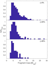Fig. 12

Normalized number of fragments in the disk vs. fragment mass in the ξ = 5% model (top panel), ξ = 50% model (middle panel), and ξ = 95% model (bottom panel). The normalization is performed on the peak value of the distribution function of fragment masses.

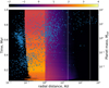Fig. 13

Comparison of the orbital positions of known exoplanets with the spatial distribution of grown dust as predicted by our numerical hydrodynamics models. The azimuthally averaged surface density of grown dust is plotted as a function of time using a color map. The scale bar on the top shows Σ_d,gr in log g cm⁻². The orbital positions of known exoplanets¹ are indicated with the blue circles as a function of their mass. The vertical dotted lines delineate the disk region where gas giants can be formed via gravitational fragmentation.

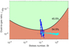Fig. 14

Regions in the ζ_d2g–St phase space that are subject to the development of a streaming instability (in green) and that are stable against a streaming instability (in brown). The corresponding data are taken from Yang et al. (2017). The blue dots present our data for the ξ = 5% model and the numbers show the percentage of time spent by this model in the unstable and stable regimes. The cyan dots present the corresponding data for the ξ = 95% model.

5.5 Models of lower mass pre-stellar cores

The mass of the pre-stellar core M_core in the models considered in the previous sections was set equal to 1.03 M_⊙, i.e., approximately to one solar mass. We only varied the rate of mass transport through the CSC defined by the ξ-parameter. It is, however, important to know how sensitive our conclusions may be to the choice of the mass of the pre-stellar core. In this section, we consider another three models characterized by similar values of the ξ-parameters (5, 50, and 95%), but having a two times smaller mass of the pre-stellar core M_core = 0.5 M_⊙.

Figure 15 presents the gas surface densities at several time instances for the three models with a lower mass of the pre-stellar core. In particular the left, middle, and right columns present the images for the ξ = 5%, ξ = 50%, and ξ = 95% models, respectively.Clearly, the main evolutionary trends discussed in the context of the one-solar-mass models (see Fig. 8) hold for the M_core = 0.5 M_⊙ models as well. The disk in the ξ = 5% model demonstrates the presence of gravitational instability to the end of numerical simulations (1.0 Myr), while the disks in the other models become virtually axisymmetric after 0.3 Myr of evolution. All three models, however, are strongly gravitationally unstable in the initial stages of disk formation and evolution (t≲100 kyr).

To further analyze the disk propensity to gravitational fragmentation in the lower-core-mass models, we plot in Fig. 16 the number of fragments that exist in the disk as a function of time in the ξ = 5% model (top panel) and ξ = 95% model (bottom panel). A comparison to Fig. 10 showing the number of fragments in the corresponding higher-core-mass models indicates that the lower-core-mass models have a systematically smaller numbers of fragments, suggesting less efficient disk fragmentation than in the higher-core-mass case. This is not surprising considering that the disk masses in the lower-core-mass models are lower by several factors. For instance, the disk mass in the ξ = 95% model at the end of numerical simulations is 0.12 M_⊙ in the higher-core-mass case and is 0.04 M_⊙ in the lower-core-mass case. What is important is that the episodic fragmentation mode, which was extensively discussed in the context of Fig. 11 for the higher-core-mass case, also exists in the lower-core-mass regime, albeit less expressed. A short episode of disk fragmentation is seen in the ξ = 5% model around t = 550 kyr, well after the onset of the T Tauri phase shown by the vertical dashed line.

Finally, the mass accretion and total stellar luminosity versus time for the low-core-mass models are presented inFig. 17. Clearly, the character of mass accretion and stellar luminosity is qualitatively similar to that discussed in the context of higher-core-mass models (see Fig. 6). The ξ = 5% model shows a highly variable accretion with episodic bursts in the early stages of evolution, while the ξ = 95% model is characterized by slowly varying accretion, but systematically higher accretion and stellar luminosity. These qualitative differences in the character of accretion and luminosity between models with different rates of mass transport through the CSC are expected to have important repercussions for the chemical evolution of protoplanetary disks (e.g., Molyarova et al. 2018).

Fig. 15

Similar to Fig. 8, but the mass of the pre-stellar core is two times lower.

Fig. 16

Similar to Fig. 10, but the mass of the pre-stellar core is two times lower.

Fig. 17

Similar to Fig. 6, but the mass of the pre-stellar core is two times lower.

6 Conclusions

We studied numerically the global evolution of viscous and self-gravitating circumstellar disks starting from disk formation and ending after about one million years of disk evolution. Such long integration times were made possible thanks to the use of the numerical hydrodynamics code FEOSAD, originally developed by Vorobyov et al. (2018) and modified in this work to include the effect of back-reaction of dust on gas according to the method laid out in Stoyanovskaya et al. (2018). The turbulent viscosity in the disk is parameterized by a spatially and temporarily constant value of the Shakura-Sunyaev α-parameter, set equal to 0.01, which corresponds to the active MRI through the disk extent. Disk self-gravity is calculated via the solution of the Poisson integral.

The inner 1.0 au of the disk is replaced with the CSC, which is a toy model that simulates physical processes that may occur in this region. These processes include mass transport from the active disk on the nascent star and MRI-triggered accretion bursts. In this work we focused on one key point: the dependence of the entire disk evolution on the mass transport rate through the CSC, which is characterized in our models by the ξ-parameter. A low value of ξ = 5% implies a slow transport of matter through the CSC on the nascent protostar, while a high value of ξ = 95% means a fast transport.

Our findings can be summarized as follows:

The evolution of gravitoviscous disks is sensitive to the rate of mass transport through the CSC. More specifically, a slow mass transport rate through the CSC (ξ = 5%) leads to the formation of more massive and warmer gaseous disks in comparison to models with a faster mass transport (ξ = 50% and ξ = 95%). The maximum size of dust grains is larger in the ξ = 5% model, reaching a decimeter radius. This model also shows an unexpectedly low dust-to-gas mass ratio in the regions between 1 au and 10 au, where it can be factors of several lower than the standard 1:100 value. We argue that this is an effect of gas accumulation in the inner disk, rather than dust depletion.
The character of mass accretion on the nascent protostar is notably affected by the rate of mass transport through the CSC. In the ξ = 95% models, the mass accretion rate steadily declines with time with only low-amplitude flickering, while in the ξ = 5% models it is highly time-variable with episodic bursts caused by the MRI triggering in the CSC. This difference can have important consequences for the dynamical and chemical evolution of the disk. On the one hand, the disk temperature for a steadily declining accretion is on average higher than for a time-variable accretion with episodic bursts. On the other hand, the bursts can raise the disk temperature by a factor of several, thus driving chemistry cycles that may be otherwise absent in the disk (e.g., Molyarova et al. 2018). We conclude that our results are robust at least for pre-stellar core masses lying in the 0.5−1.0 M_⊙ limits.
In the model with slow mass transport through the CSC (ξ = 5%) we identified a new mode of episodic disk fragmentation, which occurs in the early T Tauri phase and alternates with longer quiescent periods of disk stability. The masses of fragments formed through disk fragmentation lie in the 2–30 M_Jup limits with a maximum at 4–6 M_Jup. In general, disks are gravitationally unstable in the embedded phase of evolution, but appear nearly axisymmetric in the T Tauri phase, apart from short-lived episodes of instability, which may be statistically difficult to detect.
Grown dust efficiently drifts inward leading to the accumulation of dust in the CSC, so that the highest dust surface densities are found in the inner unresolved 1.0 au of the disk. The dust-to-gas ratios and the Stokes numbers in this region reach their limits when the streaming instability is likely to become operational. We argue that the observed diversity of exoplanets may be explained by two planet-forming mechanisms working concurrently: a streaming instability operating in the innermost disk (together with the core accretion scenario) and gravitational fragmentation operating in the outer disk regions.
Our main conclusions hold for protoplanetary disks formed from collapsing pre-stellar cores with the initial mass lying at least in the 0.5–1.0 M_⊙ limits. A study is underway to determine the robustness of our results for a wider parameter space.

In follow-up studies, we plan to address the effects of a varying α-parameter, focusing on the evolution of MRI-suppressed and MRI-dead disks. We will also consider the effects that disk photoevaporation and the varying efficiency of mass ejection via the jets may have on the disk evolution.

Acknowledgements

The authors would like to thank the anonymous referee and Beibei Liu for their comments that helped improve the manuscript. This work was supported by the Russian Science Foundation grant 17-12-01168. A.M.S. acknowledges the OeAD (Austrian Agency for International Cooperation in Education and Research) for an Ernst Mach travel grant for visiting the University of Vienna. V.G.E. acknowledges the Swedish Institute for a travel grant allowing V.G.E to visit Lund University. The simulations were performed on the Vienna Scientific Cluster. We thank Olga Stoyanovskaya and Dmitri Ionov for fruitful discussions.

References

Bae, J., Hartmann, L., Zhu, Z., & Nelson, R. P. 2014, ApJ, 795, 61 [NASA ADS] [CrossRef] [Google Scholar]
Baraffe, I., Elbakyan, V. G., Vorobyov, E. I., & Chabrier, G. 2017, A&A, 597, A19 [NASA ADS] [CrossRef] [EDP Sciences] [Google Scholar]
Basu, S. 1997, ApJ, 485, 240 [CrossRef] [Google Scholar]
Birnstiel, T., Fang, M., & Johansen, A. 2016, Space Sci. Rev., 205, 41 [NASA ADS] [CrossRef] [Google Scholar]
Boss, A. P. 2003, ApJ, 599, 577 [NASA ADS] [CrossRef] [Google Scholar]
Colella, P., & Woodward, P. R. 1984, J. Comput. Phys., 54, 174 [NASA ADS] [CrossRef] [MathSciNet] [Google Scholar]
Crida, A., Morbidelli, A., & Masset, F. 2007, A&A, 461, 1173 [NASA ADS] [CrossRef] [EDP Sciences] [Google Scholar]
Dubrulle, B., Morfill, G., & Sterzik, M. 1995, Icarus, 114, 237 [NASA ADS] [CrossRef] [Google Scholar]
Elbakyan, V. G., Vorobyov, E. I., Rab, C., et al. 2019, MNRAS, 484, 146 [NASA ADS] [CrossRef] [Google Scholar]
Evans, II, N. J., Dunham, M. M., Jørgensen, J. K., et al. 2009, ApJS, 181, 321 [NASA ADS] [CrossRef] [Google Scholar]
Forgan, D., & Rice, K. 2011, MNRAS, 417, 1928 [NASA ADS] [CrossRef] [Google Scholar]
Hubber, D. A., Walch, S., & Whitworth, A. P. 2013, MNRAS, 430, 3261 [NASA ADS] [CrossRef] [Google Scholar]
Johansen, A., Oishi, J. S., Mac Low, M.-M., et al. 2007, Nature, 448, 1022 [Google Scholar]
Kratter, K. M., Matzner, C. D., & Krumholz, M. R. 2008, ApJ, 681, 375 [NASA ADS] [CrossRef] [Google Scholar]
Machida, M. N., Inutsuka, S.-i., & Matsumoto, T. 2014, MNRAS, 438, 2278 [NASA ADS] [CrossRef] [Google Scholar]
Marleau, G.-D., Coleman, G. A. L., Leleu, A., & Mordasini, C. 2019, A&A, 624, A20 [NASA ADS] [CrossRef] [EDP Sciences] [Google Scholar]
Mayer, L., Lufkin, G., Quinn, T., & Wadsley, J. 2007, ApJ, 661, L77 [NASA ADS] [CrossRef] [Google Scholar]
Meru, F. 2015, MNRAS, 454, 2529 [NASA ADS] [CrossRef] [Google Scholar]
Meyer, D. M.-A., Vorobyov, E. I., Kuiper, R., & Kley, W. 2017, MNRAS, 464, L90 [NASA ADS] [CrossRef] [Google Scholar]
Molyarova, T., Akimkin, V., Semenov, D., et al. 2018, ApJ, 866, 46 [NASA ADS] [CrossRef] [Google Scholar]
Nayakshin, S. 2017, PASA, 34, e002 [NASA ADS] [CrossRef] [Google Scholar]
Ohtani, T., Kimura, S. S., Tsuribe, T., & Vorobyov, E. I. 2014, PASJ, 66, 112 [NASA ADS] [CrossRef] [Google Scholar]
Pringle, J. E. 1981, ARA&A, 19, 137 [NASA ADS] [CrossRef] [Google Scholar]
Rice, W. K. M., Lodato, G., Pringle, J. E., Armitage, P. J., & Bonnell, I. A. 2004, MNRAS, 355, 543 [NASA ADS] [CrossRef] [Google Scholar]
Shakura, N. I., & Sunyaev, R. A. 1973, A&A, 24, 337 [NASA ADS] [Google Scholar]
Stamatellos, D. 2015, ApJ, 810, L11 [NASA ADS] [CrossRef] [Google Scholar]
Stamatellos, D., & Whitworth, A. P. 2009, MNRAS, 392, 413 [Google Scholar]
Stamatellos, D., Whitworth, A. P., & Hubber, D. A. 2011, ApJ, 730, 32 [NASA ADS] [CrossRef] [Google Scholar]
Stoyanovskaya, O. P., Vorobyov, E. I., & Snytnikov, V. N. 2018, Astron. Rep., 62, 455 [NASA ADS] [CrossRef] [Google Scholar]
Vorobyov, E. I. 2010, ApJ, 713, 1059 [NASA ADS] [CrossRef] [Google Scholar]
Vorobyov, E. I. 2013, A&A, 552, A129 [NASA ADS] [CrossRef] [EDP Sciences] [Google Scholar]
Vorobyov, E. I. 2016, A&A, 590, A115 [NASA ADS] [CrossRef] [EDP Sciences] [Google Scholar]
Vorobyov, E. I., & Basu, S. 2005, ApJ, 633, L137 [NASA ADS] [CrossRef] [Google Scholar]
Vorobyov, E. I., & Basu, S. 2009, MNRAS, 393, 822 [NASA ADS] [CrossRef] [Google Scholar]
Vorobyov, E. I., & Basu, S. 2010, ApJ, 719, 1896 [NASA ADS] [CrossRef] [Google Scholar]
Vorobyov, E. I., & Basu, S. 2015, ApJ, 805, 115 [NASA ADS] [CrossRef] [Google Scholar]
Vorobyov, E. I., & Pavlyuchenkov, Y. N. 2017, A&A, 606, A5 [NASA ADS] [CrossRef] [EDP Sciences] [Google Scholar]
Vorobyov, E. I., & Elbakyan, V. G. 2018, A&A, 618, A7 [NASA ADS] [CrossRef] [EDP Sciences] [Google Scholar]
Vorobyov, E. I., Akimkin, V., Stoyanovskaya, O., Pavlyuchenkov, Y., & Liu, H. B. 2018, A&A, 614, A98 [NASA ADS] [CrossRef] [EDP Sciences] [Google Scholar]
Yang, C.-C., Johansen, A., & Carrera, D. 2017, A&A, 606, A80 [NASA ADS] [CrossRef] [EDP Sciences] [Google Scholar]
Yang, C.-C., Mac Low, M.-M., & Johansen, A. 2018, ApJ, 868, 27 [NASA ADS] [CrossRef] [Google Scholar]
Yorke, H. W., & Bodenheimer, P. 2008, in Massive Star Formation: Observations Confront Theory, eds. H. Beuther, H. Linz, & T. Henning, ASP Conf. Ser., 387, 189 [NASA ADS] [Google Scholar]
Zhao, B., Caselli, P., Li, Z.-Y., & Krasnopolsky, R. 2018, MNRAS, 473, 4868 [NASA ADS] [CrossRef] [Google Scholar]
Zhu, Z., Hartmann, L., Gammie, C., & McKinney, J. C. 2009, ApJ, 701, 620 [NASA ADS] [CrossRef] [Google Scholar]

¹

Taken from http://exoplanet.eu

All Figures

	Fig. 1 Graphical representation of the central smart cell (CSC) in the general context of the protostellar disk model. The main mass transport rates through the CSC are indicated with the arrows.
In the text

Fig. 2

Temporal evolution of the azimuthally averaged gas surface density (top row), grown dust surface density (second row), gas pressure (third row), gas temperature (fourth row), maximum radius ofgrown dust (fifth row), and the dust-to-gas mass ratio (bottom row) in models with ξ = 5% (left column), ξ = 50% (middle column), and ξ = 95% (right column). Contour lines indicate gas surface densities of 10³ g cm⁻² (top row), grown dust surface densities of 10 g cm⁻² (second row), and gas temperatures of 1000 K to emphasize evolutionary trends. The horizontal dotted lines in the fifth row indicatethe disk formation instance.

In the text

	Fig. 3 Radial profiles of the azimuthally averaged maximum radius of dust grains and fragmentation limit shown with the blue and orange lines, respectively. Top panel: model with ξ = 95%. Bottom panel: model with ξ = 5%.
In the text

	Fig. 4 Evolution of the dust-to-gas mass ratio in the CSC. The blue and orange lines correspond to the ξ = 5% and ξ = 95% models, respectively.
In the text

	Fig. 5 Total gas plus dust mass in the disk and stellar mass (top panel) and the mass of grown dust in the disk (bottom panel) in models with ξ = 5% (blue lines) and ξ = 95% (orange lines).
In the text

	Fig. 6 Accretion rate (top panel) and total stellar luminosity (bottom panel) for the ξ = 5% model (blue lines) and ξ = 95% model (orange lines).
In the text

Fig. 7

Top row: spatial maps of the gas temperature in the inner 600 × 600 au² box before an accretion burst (left panel), during the burst (middle panel), and after the burst (right panel) for the ξ = 5% model. Bottom row: spatial maps of the gas temperature in the ξ = 95% model characterized by steady accretion without bursts. The same evolutionary times as for the ξ = 5% model are shown. The inset plots in the right column present the azimuthally averaged temperature on the same spatial scale as the 2D temperature maps. The scale bar is in log Kelvin.

In the text

	Fig. 8 Gas surface density maps in the inner 250 × 250 au² box shown at consecutive evolutionary times for all three models with distinct ξ-parameters. Time is indicated in the left column and is counted from the onset of numerical simulations and the disk forms at 56 kyr. The scale bar is in log g cm⁻².
In the text

	Fig. 9 Global Fourier amplitudes. The solid and dashed lines correspond to models with slow (ξ = 5%) and fast (ξ = 95%) mass transport through the CSC, respectively. Shown are the Fourier amplitudes for the first three modes: m = 1, m = 2, and m = 3 in red, blue,and black, respectively.
In the text

Fig. 10

Total number of fragments present in the entire disk as a function of time in the ξ = 5% model (top panel), ξ = 50% model (middle panel), and ξ = 95% model (bottom panel). The vertical dashed lines indicate the onset of the Class II phase of disk evolution. Pink zones correspond to time periods in the Class II phase when fragments exist in the disk, and yellow zones show the time periods without any fragments in the disk. The red lines show ${\bar{Q}}_{min}$ $\overline Q_{\textrm{min}}$ , the mean minimum Toomre parameter in the disk.

In the text

Fig. 11

Gas surface density maps in the inner 600 × 600 au² box shown during a short time period between 530 kyr and 635 kyr for the ξ = 95% model (top panels) and ξ = 5% model (bottom panels). The black contour lines outline the disk regions where the Toomre Q-parameter is smaller than unity. The time is counted from the onset of numerical simulations. The disk is formed at 56 kyr. The scale bar is in log g cm⁻².

In the text

	Fig. 12 Normalized number of fragments in the disk vs. fragment mass in the ξ = 5% model (top panel), ξ = 50% model (middle panel), and ξ = 95% model (bottom panel). The normalization is performed on the peak value of the distribution function of fragment masses.
In the text

Fig. 13

Comparison of the orbital positions of known exoplanets with the spatial distribution of grown dust as predicted by our numerical hydrodynamics models. The azimuthally averaged surface density of grown dust is plotted as a function of time using a color map. The scale bar on the top shows Σ_d,gr in log g cm⁻². The orbital positions of known exoplanets¹ are indicated with the blue circles as a function of their mass. The vertical dotted lines delineate the disk region where gas giants can be formed via gravitational fragmentation.

In the text

Fig. 14

Regions in the ζ_d2g–St phase space that are subject to the development of a streaming instability (in green) and that are stable against a streaming instability (in brown). The corresponding data are taken from Yang et al. (2017). The blue dots present our data for the ξ = 5% model and the numbers show the percentage of time spent by this model in the unstable and stable regimes. The cyan dots present the corresponding data for the ξ = 95% model.

In the text

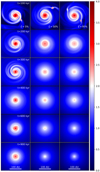	Fig. 15 Similar to Fig. 8, but the mass of the pre-stellar core is two times lower.
In the text

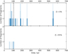	Fig. 16 Similar to Fig. 10, but the mass of the pre-stellar core is two times lower.
In the text

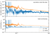	Fig. 17 Similar to Fig. 6, but the mass of the pre-stellar core is two times lower.
In the text

Current usage metrics show cumulative count of Article Views (full-text article views including HTML views, PDF and ePub downloads, according to the available data) and Abstracts Views on Vision4Press platform.

Data correspond to usage on the plateform after 2015. The current usage metrics is available 48-96 hours after online publication and is updated daily on week days.

Initial download of the metrics may take a while.

[1] Bae, J., Hartmann, L., Zhu, Z., & Nelson, R. P. 2014, ApJ, 795, 61 [NASA ADS] [CrossRef] [Google Scholar]

[2] Baraffe, I., Elbakyan, V. G., Vorobyov, E. I., & Chabrier, G. 2017, A&A, 597, A19 [NASA ADS] [CrossRef] [EDP Sciences] [Google Scholar]

[3] Basu, S. 1997, ApJ, 485, 240 [CrossRef] [Google Scholar]

[4] Birnstiel, T., Fang, M., & Johansen, A. 2016, Space Sci. Rev., 205, 41 [NASA ADS] [CrossRef] [Google Scholar]

[5] Boss, A. P. 2003, ApJ, 599, 577 [NASA ADS] [CrossRef] [Google Scholar]

[6] Colella, P., & Woodward, P. R. 1984, J. Comput. Phys., 54, 174 [NASA ADS] [CrossRef] [MathSciNet] [Google Scholar]

[7] Crida, A., Morbidelli, A., & Masset, F. 2007, A&A, 461, 1173 [NASA ADS] [CrossRef] [EDP Sciences] [Google Scholar]

[8] Dubrulle, B., Morfill, G., & Sterzik, M. 1995, Icarus, 114, 237 [NASA ADS] [CrossRef] [Google Scholar]

[9] Elbakyan, V. G., Vorobyov, E. I., Rab, C., et al. 2019, MNRAS, 484, 146 [NASA ADS] [CrossRef] [Google Scholar]

[10] Evans, II, N. J., Dunham, M. M., Jørgensen, J. K., et al. 2009, ApJS, 181, 321 [NASA ADS] [CrossRef] [Google Scholar]

[11] Forgan, D., & Rice, K. 2011, MNRAS, 417, 1928 [NASA ADS] [CrossRef] [Google Scholar]

[12] Hubber, D. A., Walch, S., & Whitworth, A. P. 2013, MNRAS, 430, 3261 [NASA ADS] [CrossRef] [Google Scholar]

[13] Johansen, A., Oishi, J. S., Mac Low, M.-M., et al. 2007, Nature, 448, 1022 [Google Scholar]

[14] Kratter, K. M., Matzner, C. D., & Krumholz, M. R. 2008, ApJ, 681, 375 [NASA ADS] [CrossRef] [Google Scholar]

[15] Machida, M. N., Inutsuka, S.-i., & Matsumoto, T. 2014, MNRAS, 438, 2278 [NASA ADS] [CrossRef] [Google Scholar]

[16] Marleau, G.-D., Coleman, G. A. L., Leleu, A., & Mordasini, C. 2019, A&A, 624, A20 [NASA ADS] [CrossRef] [EDP Sciences] [Google Scholar]

[17] Mayer, L., Lufkin, G., Quinn, T., & Wadsley, J. 2007, ApJ, 661, L77 [NASA ADS] [CrossRef] [Google Scholar]

[18] Meru, F. 2015, MNRAS, 454, 2529 [NASA ADS] [CrossRef] [Google Scholar]

[19] Meyer, D. M.-A., Vorobyov, E. I., Kuiper, R., & Kley, W. 2017, MNRAS, 464, L90 [NASA ADS] [CrossRef] [Google Scholar]

[20] Molyarova, T., Akimkin, V., Semenov, D., et al. 2018, ApJ, 866, 46 [NASA ADS] [CrossRef] [Google Scholar]

[21] Nayakshin, S. 2017, PASA, 34, e002 [NASA ADS] [CrossRef] [Google Scholar]

[22] Ohtani, T., Kimura, S. S., Tsuribe, T., & Vorobyov, E. I. 2014, PASJ, 66, 112 [NASA ADS] [CrossRef] [Google Scholar]

[23] Pringle, J. E. 1981, ARA&A, 19, 137 [NASA ADS] [CrossRef] [Google Scholar]

[24] Rice, W. K. M., Lodato, G., Pringle, J. E., Armitage, P. J., & Bonnell, I. A. 2004, MNRAS, 355, 543 [NASA ADS] [CrossRef] [Google Scholar]

[25] Shakura, N. I., & Sunyaev, R. A. 1973, A&A, 24, 337 [NASA ADS] [Google Scholar]

[26] Stamatellos, D. 2015, ApJ, 810, L11 [NASA ADS] [CrossRef] [Google Scholar]

[27] Stamatellos, D., & Whitworth, A. P. 2009, MNRAS, 392, 413 [Google Scholar]

[28] Stamatellos, D., Whitworth, A. P., & Hubber, D. A. 2011, ApJ, 730, 32 [NASA ADS] [CrossRef] [Google Scholar]

[29] Stoyanovskaya, O. P., Vorobyov, E. I., & Snytnikov, V. N. 2018, Astron. Rep., 62, 455 [NASA ADS] [CrossRef] [Google Scholar]

[30] Vorobyov, E. I. 2010, ApJ, 713, 1059 [NASA ADS] [CrossRef] [Google Scholar]

[31] Vorobyov, E. I. 2013, A&A, 552, A129 [NASA ADS] [CrossRef] [EDP Sciences] [Google Scholar]

[32] Vorobyov, E. I. 2016, A&A, 590, A115 [NASA ADS] [CrossRef] [EDP Sciences] [Google Scholar]

[33] Vorobyov, E. I., & Basu, S. 2005, ApJ, 633, L137 [NASA ADS] [CrossRef] [Google Scholar]

[34] Vorobyov, E. I., & Basu, S. 2009, MNRAS, 393, 822 [NASA ADS] [CrossRef] [Google Scholar]

[35] Vorobyov, E. I., & Basu, S. 2010, ApJ, 719, 1896 [NASA ADS] [CrossRef] [Google Scholar]

[36] Vorobyov, E. I., & Basu, S. 2015, ApJ, 805, 115 [NASA ADS] [CrossRef] [Google Scholar]

[37] Vorobyov, E. I., & Pavlyuchenkov, Y. N. 2017, A&A, 606, A5 [NASA ADS] [CrossRef] [EDP Sciences] [Google Scholar]

[38] Vorobyov, E. I., & Elbakyan, V. G. 2018, A&A, 618, A7 [NASA ADS] [CrossRef] [EDP Sciences] [Google Scholar]

[39] Vorobyov, E. I., Akimkin, V., Stoyanovskaya, O., Pavlyuchenkov, Y., & Liu, H. B. 2018, A&A, 614, A98 [NASA ADS] [CrossRef] [EDP Sciences] [Google Scholar]

[40] Yang, C.-C., Johansen, A., & Carrera, D. 2017, A&A, 606, A80 [NASA ADS] [CrossRef] [EDP Sciences] [Google Scholar]

[41] Yang, C.-C., Mac Low, M.-M., & Johansen, A. 2018, ApJ, 868, 27 [NASA ADS] [CrossRef] [Google Scholar]

[42] Yorke, H. W., & Bodenheimer, P. 2008, in Massive Star Formation: Observations Confront Theory, eds. H. Beuther, H. Linz, & T. Henning, ASP Conf. Ser., 387, 189 [NASA ADS] [Google Scholar]

[43] Zhao, B., Caselli, P., Li, Z.-Y., & Krasnopolsky, R. 2018, MNRAS, 473, 4868 [NASA ADS] [CrossRef] [Google Scholar]

[44] Zhu, Z., Hartmann, L., Gammie, C., & McKinney, J. C. 2009, ApJ, 701, 620 [NASA ADS] [CrossRef] [Google Scholar]