| Issue |
A&A
Volume 627, July 2019
|
|
|---|---|---|
| Article Number | A135 | |
| Number of page(s) | 16 | |
| Section | Stellar structure and evolution | |
| DOI | https://doi.org/10.1051/0004-6361/201935418 | |
| Published online | 12 July 2019 | |
Variability of young stellar objects in the star-forming region Pelican Nebula⋆
1
Kavli Institute for Astronomy and Astrophysics, Peking University, Yi He Yuan Lu 5, Hai Dian District, Beijing 100871, PR China
e-mail: This email address is being protected from spambots. You need JavaScript enabled to view it.
, This email address is being protected from spambots. You need JavaScript enabled to view it.
2
Aryabhatta Research Institute of Observational Sciences, Manora Peak, Nainital, 263002 Uttarakhand, India
3
Graduate Institute of Astronomy, National Central University, Jhongli 32001, Taiwan
4
Department of Physics and Astrophysics, University of Delhi, Delhi 110007, India
Received:
6
March
2019
Accepted:
31
May
2019
Abstract
Context. Pre-main-sequence variability characteristics can be used to probe the physical processes leading to the formation and initial evolution of both stars and planets.
Aims. The photometric variability of pre-main-sequence stars is studied at optical wavelengths to explore star–disk interactions, accretion, spots, and other physical mechanisms associated with young stellar objects.
Methods. We observed a field of 16′ × 16′ in the star-forming region Pelican Nebula (IC 5070) at BVRI wavelengths for 90 nights spread over one year in 2012−2013. More than 250 epochs in the VRI bands are used to identify and classify variables up to V ∼ 21 mag. Their physical association with the cluster IC 5070 is established based on the parallaxes and proper motions from the Gaia second data release (DR2). Multiwavelength photometric data are used to estimate physical parameters based on the isochrone fitting and spectral energy distributions.
Results. We present a catalog of optical time-series photometry with periods, mean magnitudes, and classifications for 95 variable stars including 67 pre-main-sequence variables towards star-forming region IC 5070. The pre-main-sequence variables are further classified as candidate classical T Tauri and weak-line T Tauri stars based on their light curve variations and the locations on the color-color and color-magnitude diagrams using optical and infrared data together with Gaia DR2 astrometry. Classical T Tauri stars display variability amplitudes up to three times the maximum fluctuation in disk-free weak-line T Tauri stars, which show strong periodic variations. Short-term variability is missed in our photometry within single nights. Several classical T Tauri stars display long-lasting (≥10 days) single or multiple fading and brightening events of up to two magnitudes at optical wavelengths. The typical mass and age of the pre-main-sequence variables from the isochrone fitting and spectral energy distributions are estimated to be ≤1 M⊙ and ∼2 Myr, respectively. We do not find any correlation between the optical amplitudes or periods with the physical parameters (mass and age) of pre-main-sequence stars.
Conclusions. The low-mass pre-main-sequence stars in the Pelican Nebula region display distinct variability and color trends and nearly 30% of the variables exhibit strong periodic signatures attributed to cold spot modulations. In the case of accretion bursts and extinction events, the average amplitudes are larger than one magnitude at optical wavelengths. These optical magnitude fluctuations are stable on a timescale of one year.
Key words: stars: pre-main sequence / stars: variables: T Tauri, Herbig Ae/Be / open clusters and associations: general / stars: low-mass
Full Tables 1 and 2 are only available at the CDS via anonymous ftp to cdsarc.u-strasbg.fr (130.79.128.5) or via http://cdsarc.u-strasbg.fr/viz-bin/qcat?J/A+A/627/A135
© ESO 2019
1. Introduction
Most stars show variability in brightness during some stage of their life cycles. Photometric variability is a characteristic feature of stars in the pre-main-sequence (PMS) phase, and it provides insight into the different physical processes in young stars when studied at multiple wavelengths. Variability is a ubiquitous property of T Tauri stars (TTSs) that are low-mass (M < 2 M⊙) PMS objects (Joy 1945). Classical TTSs (CTTSs) actively accrete material from the circumstellar disks while weak-line TTSs (WTTSs) do not show any ongoing accretion perhaps due to the lack of inner disks. CTTSs exhibit large photometric variability with excess infrared and ultraviolet emission, and strong Hα emission. In contrast, WTTSs show periodic variability with smaller amplitudes, little or no infrared excess, and a smaller Hα equivalent width (Herbig 1962, 1977; Bertout 1989; Herbst et al. 1994). Herbig Ae/Be represent a more massive class of PMS stars (2 M⊙ < M < 8 M⊙) and exhibit different types of photometric variability as they evolve towards the zero age main sequence (ZAMS). Some of the massive stars that reach the main sequence (MS) in their core hydrogen burning phase also display changes in their brightness due to pulsations, for example, β Cep, δ Scuti, or slowly pulsating B stars (Eyer & Mowlavi 2008).
Optical photometric variability in young stellar objects (YSOs) is attributed to a range of physical mechanisms. Variability in WTTSs occurs due to an asymmetric distribution of cool or dark magnetic spots at the stellar surface that modulates the observed luminosity of the star during its rotation (Bouvier et al. 1993; Herbst et al. 1994; Grankin et al. 2008). In CTTSs, variability is caused by the variable accretion from the circumstellar disk onto the star, where both the accretion rate and the distribution of accretion zone or hot spots over the stellar surface are not uniform (Herbst et al. 2007; Cody et al. 2014). Variability in Herbig Ae/Be stars predominantly occurs due to the obscuration from the circumstellar dust (Bertout 1989; Herbst et al. 1994, 2007; Semkov 2011; Stelzer 2015). Since YSOs exhibit different variability signatures, exploring their variable properties at multiple wavelengths is essential to understand the complex nature of these stars on both short and long timescales.
Several studies have focussed on the PMS variability of YSOs with the aim of understanding the star–disk interactions, accretion, outflows, and other physical mechanisms (e.g., Grankin et al. 2008; Alencar et al. 2010; Venuti et al. 2015; Messina et al. 2017; Rodriguez et al. 2017; Fernandes et al. 2018; Guo et al. 2018). Space-based observations allowed a remarkable progress in YSO variability studies thanks to the high-precision photometry that probes the flux variation to 1% of amplitudes and on timescales of less then one hour (Alencar et al. 2010; Cody et al. 2014; Ansdell et al. 2016; Gillen et al. 2017). Using photometric data with unprecedented accuracy, a detailed (sub)classification of YSOs (e.g., quasi-periodic, dippers, bursters) was provided by Cody et al. (2014) based on their light curve morphology at multiple wavelengths. Venuti et al. (2015) studied the variability and accretion dynamics of YSOs in the NGC 2264 at ultraviolet and optical wavelengths and found that the accretion process is stable on timescales of years. The PMS variability could also contribute to the large scatter observed in Hertzsprung-Russell diagrams for star-forming regions (SFRs, Baraffe et al. 2009, 2012), while the correlation of the rotation period and/or amplitude with different stellar properties can potentially provide insight into the angular momentum evolution in PMS stars (Bouvier et al. 1997; Herbst et al. 2007).
The North America (NGC 7000) and Pelican (IC 5070) Nebulae are SFRs that are within one kiloparsec of the Sun. This complex provides an ideal laboratory to study the influence of massive stars on subsequent star formation activity and evolution of the natal molecular clouds (Guieu et al. 2009; Rebull et al. 2011; Zhang et al. 2014; Bally et al. 2014). These regions possess a large number of young PMS stars, cometary nebulae, bright-rimmed clouds, collimated jets, and Herbig-Haro objects (Ogura et al. 2002; Ikeda et al. 2008; Rebull et al. 2011; Panwar et al. 2014; Bally et al. 2014). Rebull et al. (2011) identified more than 2000 YSOs in the 7 deg2 field towards the North America and Pelican complex including nearly 250 YSOs in the Pelican cluster. However, the long-term optical photometric studies of PMS stars in these regions are available only for a limited sample (Kóspál et al. 2011; Findeisen et al. 2013; Poljančić et al. 2014; Ibryamov et al. 2018, and references within). The BVRI photometry for a sample of 17 PMS objects was presented by Poljančić et al. (2014) in the field of the North America and Pelican Nebulae, while Froebrich et al. (2018) found two new low-mass young stars with deep recurring eclipses in IC 5070.
In this work, we present a relatively large sample of variable YSOs in IC 5070 based on a year-long optical photometry. The paper is structured as follows. Section 2 provides details of the observations, data reduction, and photometric and astrometric calibrations. The variability identification, period determination, and a comparison with published works are discussed in Sect. 3. The classification of YSOs based on their kinematics, color-color diagrams (CCDs) and color-magnitude diagrams (CMDs), and the light curve variations are discussed in Sect. 4. A detailed discussion on the physical and variable characteristics of PMS stars is presented in Sect. 5, including the estimates of physical parameters based on the spectral energy distribution (SED) fitting tool. The final results of this work are summarized in Sect. 6.
2. Observations, data reduction, and photometric and astrometric calibrations
The observations were carried out using the 0.81 m (32′′) Tenagra telescope, which uses a science camera with 2048 × 2048 pixels having an effective plate scale of ∼0.98′′ per pixel and a field of view of 16.8 × 16.8 arcmin2. The images in the VRI filters were acquired between May 2012 and June 2013 over 90 nights, often three times each night but within one hour, while the B-band images were taken only over two nights. There are only 5 frames in B and around 250 frames in VRI, taken with exposures varying from 420s in B to 90s in I. Calibration images (bias and flats) were obtained nightly and the pre-processing of images (bias subtraction, flat-fielding, etc.) was done in IRAF1. Finally, 760 scientifically useful images were used to perform photometry. Figure 1 shows the color-composite image of the selected star-forming region towards IC 5070 obtained using the VRI images taken on the first night.
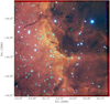 |
Fig. 1. Color composite image of the young star-forming region towards Pelican Nebula obtained using the VRI-band images. The cyan circles represent the location of the variable stars. |
The time-series photometry of the processed images was performed using DAOPHOT/ALLSTAR (Stetson 1987) and DAOMATCH/DAOMASTER (Stetson 1993) routines. In this process all sources above the 4σ threshold in each image are selected and the aperture photometry is obtained with a radius of 4 pixels. The point spread function (PSF) is determined from 20 bright and isolated stars in each image, which is used to perform the PSF photometry using ALLSTAR on all images. The frames taken on the first night are selected as the master image in each filter and the PSF photometry are used as input to DAOMATCH to derive accurate frame-to-frame coordinate transformations. These transformations are used to obtain the corrected magnitudes of the stars relative to their magnitudes in the master image for all frames using DAOMASTER. The photometry includes 1307 sources with more than 50 observations in the target field, and over 1000 stars with both V- and I-band measurements. Within our target region, optical counterparts of 77 of the ∼135 YSOs from Rebull et al. (2011) were found within 3′′ matching radius in our photometry.
The photometric calibration to Landolt filters (Landolt 2009) was performed using the standard star photometry carried out on the same night as the master frame. The standard transformation equations are:
where, b, v, r, i are instrumental magnitudes; B, V, R, I are standard magnitudes; and Xb, Xv, Xr, Xi are the airmass in the BVRI filters. The maximum uncertainty of these coefficients and the dispersion in these relations are on the order of 0.02 magnitude. If the star is observed in one filter only, the median instrumental color at the corresponding magnitude is adopted to calibrate its magnitude. The top panel of Fig. 2 shows the photometric precision of our observations as a function of I-band instrumental magnitude. For the calibrated magnitudes, the minimum uncertainty is 0.02 mag for the brightest sources and exceeds 0.05 mag for the fainter targets. The calibrated magnitudes were compared with a sample of 37 common stars with the AAVSO Photometric All Sky Survey (Henden et al. 2016) that resulted in a median absolute deviation of ∼0.2 mag in B and ∼0.1 mag in V. We also compared the BVRI magnitudes with small sample of stars compiled by Guieu et al. (2009) and Findeisen et al. (2013), and the median offset in each filter was found to be on the order of 10% of the magnitude range. The typical uncertainties on all the literature magnitudes are also on the order of one-tenth of a magnitude. The astrometric calibration was performed with ten bright and isolated sources using data from Gaia DR2 (Gaia Collaboration 2018a).
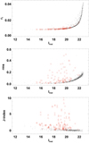 |
Fig. 2. Top panel: photometric precision of our observations in I band as a function of instrumental magnitudes. Middle panel: root mean square (rms) scatter in I band as a function of instrumental magnitudes. Red circles denote the selected candidate variables in the top and middle panels. Bottom panel: Stetson’s J-index for all sources in our field as a function of instrumental I-band magnitudes. Red circles and triangles represent the variables with light curves available in RI and VI bands. |
The five-parameter solution (astrometry, parallax, and proper motions) for all sources were obtained using a 3′′ search radius from Gaia DR2 catalog (Gaia Collaboration 2018b). Our astrometric calibration was not expected to be better than 1−2′′ and therefore all pairs within 1.5′′ were investigated to remove possible duplicates after combining data in different filters. Finally, the RA and Dec of the nearest neighbor source in the Gaia catalog were adopted for further analysis. We also obtained various physical parameters including luminosity and effective temperatures, if provided in the Gaia catalog. We note that Luri et al. (2018) has suggested using a Bayesian approach to properly account for the covariance uncertainties in the parallaxes and proper motions from Gaia DR2. Therefore, accurate distances for these sources were also adopted from the catalog of Bailer-Jones et al. (2018) that were determined using a Bayesian inference method based on a distance prior that varies smoothly as a function of Galactic longitude and latitude according to a Galaxy model. Multiband photometric data for all the sources were also obtained by a cross-match within a search radius of 3′′ to the Two Micron All Sky Survey (2MASS, Cutri et al. 2003), Spitzer, Multiband Imaging Photometer for Spitzer (MIPS), and Wide-field Infrared Survey Explorer (WISE) archival catalogs2.
3. Variability search and period determination
We considered more than 1300 stars that were observed in at least 50 frames for the variability classification and period determination. At first, the stars with large root mean square scatter around the mean magnitude from the combined multiframe data were identified as candidate variables in each filter. The dispersion around mean magnitude from the time-series data provides a measure of the intrinsic variability of a star. For variable objects, root mean square scatter is significantly larger than the photometric noise, while the fluctuations around the mean are on the order of the photometric uncertainties for the non-variable stars. Therefore, the full magnitude range is binned in different stepsizes of 0.2/0.5/1.0 mag and all stars above the 3σ level in each bin are selected as candidate variables. Only stars for which the root mean square dispersion in I band exceeds 0.05 mag are considered as variable candidates. After combining individual variables in the VRI filters, a sample of 152 candidate variables show variability in at least one filter. Furthermore, the correlated variability in different wavelengths is studied with a more robust approach using the J-index (Stetson 1996). Stetson’s J-index is calculated for stars with light curves available in the VI and RI filters using the equations
where Pk is the product of normalized residuals of N pairs of simultaneous observations and sgn is the sign function. The weight wk is adopted as the inverse of the time difference between the pair of observations. The middle and bottom panels of Fig. 2 show the rms scatter and Stetson’s J-index as a function of instrumental I-band magnitudes. Most candidate variables selected from the rms scatter also have a J-index ≥0.5 and no additional variable candidate is found based on a J-index value above this threshold.
The Lomb-Scargle periodogram (Lomb 1976; Scargle 1982), phase-dispersion minimization (Stellingwerf 1978), and analysis of variance (Schwarzenberg-Czerny 1989) methods are used to find the periods for candidate variables. These different period determination algorithms allow us to ascertain the consistency of estimated periods. The period search was carried out in 106 steps between 0.1 and 100 days. A typical uncertainty on the measured periods is found to be smaller than one-tenth of a day. A star is identified as a periodic variable if the difference between periods in any two methods is smaller than 10−3 day. The remaining light curves are further visually inspected to select variable candidates displaying periodic and/or nonperiodic variations. In cases where the variability is not observed in all three filters, we restrict the sample to stars that display at least 10% of magnitude fluctuations and the amplitude is significantly larger than the dispersion in the light curve. The final sample of variables consists of 95 stars (see Fig. 2), 56 of which show periodic variability in at least one of the VRI filters. Only 5 stars have amplitudes smaller than 0.1 mag in I band. Multi-epoch photometric data of variable sources are listed in Table 1. From Gaia DR2, 91 (out of 95) variables have parallaxes and proper motions, and 2 of these are fainter than 20 mag in G band.
Time-series VRI-band photometry of variable sources.
The variable YSO sample with long-term time-series photometry in IC 5070 is very limited (Findeisen et al. 2013; Poljančić et al. 2014; Ibryamov et al. 2018; Froebrich et al. 2018, as discussed in Sect. 1). Therefore, a number of our targets are new variable sources identified in the IC 5070. Out of the 77 stars common with Rebull et al. (2011) in our target region, only 42 exhibit variability in the final sample. The photometric properties of periodic and non-periodic variables are listed in Table 2. The rms scatter for each variable source is added in quadrature to the photometric uncertainties listed in Table 2. Figure 3 shows the representative light curves of periodic and non-periodic variables.
Properties of variable sources.
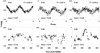 |
Fig. 3. Representative I-band light curves of periodic (top) and nonperiodic variables (bottom) with varying light curve quality. The magnitudes are normalized with respect to the zero-mean. Star ID, period, and mean magnitude are also provided in each panel. The vertical dashed line in the bottom panels separates the observations into two different seasons that are offset for visualization purposes. |
4. Classification and evolutionary stages of the variable stars
In order to classify the variable sources, it is essential to determine their association with the Pelican Nebula region. The CCDs, the CMDs, and the kinematics information are very useful when identifying stars associated with a cluster (Panwar et al. 2014; Lata et al. 2016).
4.1. Membership
The parallaxes and proper motions from Gaia DR2 are used for variable sources to identify possible members of the Pelican Nebula region. Figure 4 shows the scatterplot and histograms of proper motions for variable candidates. The Gaussian distribution fits to the proper motions along right ascension (μα) and declination (μδ) provide a mean value of −1.32 and −3.87 mas per year with a half width at half maximum of 0.65 and 0.67 mas per year, respectively. A distinct clustering in the scatterplot is visible around μα ∼ −1 mas per year and μδ ∼ −4 mas per year. The inner circle is centered at the peak values from the Gaussian distribution with a radius of 2 mas per year, equivalent to three times their half width at half maximum. Assuming the center of the radius as the proper motion of the cluster, 27 variables are found with proper motions beyond 3σ of the mean values. Of these 27 variables, 5 stars have large uncertainties on their proper motions sufficient to bring them within the inner radius. Therefore, 22 (out of 95) variables are likely MS or field stars and do not belong to the Pelican Nebula region. In addition, four stars do not have kinematic information available from Gaia data.
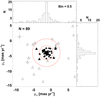 |
Fig. 4. Scatterplot of variable sources in the proper motion plane. Histograms for proper motions along right ascension and declination are also shown. The center of the circles is at the peak values of proper motions from the Gaussian distribution fits to the histograms. The inner and outer radius is of 2 and 4 mas per year, respectively. Filled circles denote kinematically selected members. Open triangles represent 3σ (∼2 mas per year) outliers from the mean of the Gaussian distribution fits to the histograms of the proper motions. Filled triangles display variables for which the proper motions are consistent with the mean value given their 3σ uncertainties. The bin size used in the histograms and the number of stars shown are indicated at the top. |
Figure 5 displays the scatterplot of parallaxes against the proper motions for variable candidates. In the parallax histogram, the Gaussian distribution peaks at 1.21 mas with a half width at half maximum of 0.15 mas, corresponding to a median distance of 826.5 pc with 1σ standard deviation of 101.6 pc, for all the target variables in our analysis. Four stars have negative parallaxes and the distances for 82 (out of 91) variables are consistent with the mean value given their uncertainties. To estimate a robust distance to the IC 5070, we iteratively exclude stars that have kinematics and distances beyond 3σ of their mean values. The stars with excess astrometric noise of more than 2 mas are also excluded from this analysis. For the remaining sample of 59 stars, individual distances and their associated uncertainties are used from the catalog of Bailer-Jones et al. (2018) to perform bootstrapping. We create 104 random realizations by perturbing the uncertainties in each iteration and finally fit a Gaussian distribution to estimate a distance of 857.5 ± 55.8 pc to the IC 5070. The distance estimates to the Pelican Nebula region vary from 500 pc to over 1 kpc, but a distance closer to 600 pc is preferred with a typical uncertainty of 10% (Laugalys et al. 2007; Reipurth & Schneider 2008; Guieu et al. 2009). This commonly adopted distance is based on the extensive multicolor photometry that is used to determine color excesses, extinction, and distances for hundreds of stars towards the Pelican Nebula region (Laugalys et al. 2007, and references within).
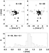 |
Fig. 5. Top panel: scatterplot of parallaxes against the proper motions along right ascension and declination. The symbols are the same as in Fig. 4. Bottom panel: histogram of parallaxes for variable sources from the Gaia DR2. The bin size used in the histogram and the number of stars shown in the plots are indicated at the top. |
4.2. Color-magnitude and color-color diagrams
Optical color-magnitude and near-infrared (NIR) color-color diagrams are used to classify our variable candidates. The 2MASS JHKs data are available for 93 stars, while for the remaining two stars, photometric data are adopted from the UKIDSS Galactic Plane Survey (Lucas et al. 2008). The 2MASS photometry is transformed to the California Institute of Technology (CIT) system using the relations provided on their website3 to compare with the evolutionary models. Figure 6 represents the J − H/H − K CCD based on 2MASS data, typically used to classify the YSOs. The YSOs from Rebull et al. (2011) and Ogura et al. (2002) are overplotted in colored symbols. The sequence of dwarf and giants from Bessell & Brett (1988), and the intrinsic locus of CTT stars (Meyer et al. 1997) are also overplotted. The three parallel lines are the reddening vectors drawn from the tip of the giant branch (left), from the base of the MS branch (middle), and from the tip of the intrinsic CTTSs line (right). The extinction ratios to derive these reddening vectors are  , adopted from Cohen et al. (1981). In general, CTTSs with smaller NIR excess, WTTSs, and field stars (MS and giants) occupy the region between the left and middle reddening vectors. Figure 6 shows that most of the variables that are outliers in the proper motions and lie below the intrinsic CTTSs locus are the MS stars. Two variables (V173 and V177) are members based on their proper motions, but fall below the giant sequence. One of these, V173, does not have kinematic information. The CTTSs with large infrared excess are located in the region between the middle and right reddening vectors, while more moderate CTTSs with smaller infrared excess can also populate the region between left and middle reddening vectors, mixed with reddened WTTSs just above the CTT locus. Some contamination is expected depending on the reddening and IR excess, and also due to variability in single-epoch measurements.
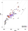 |
Fig. 6. Near-infrared CCD for all variables. The solid curve and dotted curve represent the sequence of dwarf and giants from Bessell & Brett (1988). The locus of CTT stars is shown as long-dashed lines (Meyer et al. 1997), while the dot-dashed lines represent the reddening vectors (Cohen et al. 1981). Diamonds and open triangles represent the kinematic members and outliers, respectively. The solid arrow indicates reddening vector corresponding to AV = 5 mag. Each star is numbered with the last two digits of the Star ID from Table 2. |
The optical V/V − I CMD is a useful tool for ascertaining the evolutionary status of variables and their probable cluster membership. Figure 7 shows the CMD for the variable candidates. The theoretical isochrones of 0.1, 1, 5, and 10 Myr and evolutionary tracks of various masses for PMS stars are plotted from Siess et al. (2000). We also plotted the ZAMS with the solar metal abundance (Z = 0.02) from Girardi et al. (2002). The isochrones and evolutionary tracks are corrected for a distance of 857.5 pc to the cluster and for the average extinction of AV = 1.9 mag. The average extinction is estimated by tracing back the location of all variables on the NIR CCD to the intrinsic locus along the reddening vector. The value of AV varies between zero and ten mag for these variables. The reddening towards the young stars is often differential across the star-forming region and a larger spread in reddening is expected throughout the cluster, as shown in the extinction maps by Cambrésy et al. (2002) based on 2MASS colors. The individual AV measurements may suffer from the possible degeneracies when the spectral information is not available, and in some cases the adopted average extinction may also be offset with respect to optical colors. The extinction measurements may differ from NIR estimates even if the spectral type is known (Herczeg & Hillenbrand 2014). However, the average extinction based on NIR colors displays a reasonable fit to the PMS population in the optical CCD in our sample. Again, most of the proper motion outliers appear along the ZAMS in Fig. 7 except five variables (V116, V117, V140, V141, and V142) that follow a younger PMS population. The light curves in V band for V141 and V142 are of poor quality, and it is possible that either the colors or magnitudes for all these objects are spurious, leading to an offset towards a younger population.
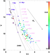 |
Fig. 7. Apparent optical V/V − I CMD for the variable candidates. The dashed curve shows the isochrones for PMS stars with different ages from Siess et al. (2000), while the solid curve is the ZAMS by Girardi et al. (2002). The dotted curves display the evolutionary tracks of PMS stars with different stellar masses. The isochrones and the evolutionary tracks are offset with respect to the average distance (857.5 pc) and extinction (AV = 1.9 mag). The color bar represents the 2MASS (H − K) color. Open triangles represent the kinematic outliers. The arrow indicates the direction of the reddening vector corresponding to AV = 5 mag. |
The age and mass of variable candidates are estimated by comparing their locations in the observed CMD with the theoretical PMS isochrones of Siess et al. (2000) and Bressan et al. (2012). There are several obvious reasons why these estimates are likely to be uncertain, for example, isochrones uncertainties, lack of precise reddening corrections, and binarity and variability effects on colors. In order to provide an accurate range of age and mass estimates, a single distance of 857.5 ± 55.8 pc and an extinction of AV = 1.9 mag is adopted to offset absolute magnitudes. The isochrones and evolutionary tracks on the CMD are interpolated using a two-dimensional grid. First, the unevenly spaced isochrones and evolutionary tracks are trianglulated to form a regular grid. Then the age and mass estimates are obtained for each star on the observed CMD by interpolating the two-dimensional regular grid using inverse distance weighted interpolation (i.e., the nearest age and mass grid to the data points in the CMD are given higher weights). In order to have a more robust estimate, the errors in photometry, distances, and reddening are added in quadrature to perform a bootstrapping by allowing the magnitude and colors to change within 1σ. Several (104) random realizations are created and the median values of the age and mass are adopted as final estimates, while the standard deviation as the error on the adopted values. Table 3 lists the age and mass estimates from the isochrone fitting to the CMD for those variables that have V & I measurements and have accurate parallaxes. Most stars have masses less than 2 M⊙ and ages less than 10 Myr with a median uncertainty of 9% and 24% on mass and age estimates, respectively. Additionally, individual distances from the catalog of Bailer-Jones et al. (2018) are used to estimate the absolute V-band magnitude for our variables and perform the same analysis. From Table 3, the difference in the masses and ages between these two approaches are typically smaller than their quoted uncertainties. However, masses for seven stars and the ages for ten stars in our sample differ by more than 3σ of their uncertainties in the single cluster distance approach.
Age and mass estimates of variable stars based on isochrone fitting.
Theoretical isochrones from Bressan et al. (2012) are also used for a systematic comparison and a median difference of ∼16% is noted for masses greater than 0.6 M⊙. However, low-mass (≤0.6 M⊙) evolutionary tracks from Bressan et al. (2012) display a systematic offset with respect to Siess et al. (2000) and the median difference in the estimated masses is around 29%. Similar differences are also found in age estimates for the popoulation younger than 1 Myr, but the two sets of age estimates from different theoretical isochrones are consistent given their large uncertainties. Typically, the masses inferred for individual stars from theoretical models are accurate to better than 10% for masses >1 M⊙, but are highly discrepant for subsolar masses (Stassun et al. 2014; David et al. 2019). Similarly, the systematic differences between ages predicted with different theoretical isochrones increase towards younger ages and for lower masses (Hillenbrand et al. 2008; Soderblom et al. 2014). With adopted distance and extinction to the IC 5070 cluster, a median mass and age of ∼0.82 M⊙ and 1.55 Myr is found based on the isochrone fitting to the observed CMD. Figure 8 displays the K/I − K CMD for variable sources with different stellar masses and ages where the MS or field variables are distinctly separated from younger PMS stars.
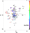 |
Fig. 8. K/I − K CMD. The stars are numbered with the last two digits of their Star ID from Table 2. The color bar represents the age determined from the isochrone fitting. Open triangles represent the kinematic outliers. The arrow indicates the reddening vector corresponding to AV = 5 mag. The increase in symbol size represents the increase in mass obtained from the evolutionary tracks. |
4.3. Classification of variables
In addition to the proper motions, distances, and the CCDs and CMDs, we use the light curve structure to classify the variables in different subclasses. All the kinematic outliers (22 stars) are classified as MS or field stars; a few additional variables (6 stars including 2 distance outliers) are also classified as MS stars as they fall below the giant sequence on the NIR CCD or follow the ZAMS in the optical CMD. The rest of the PMS stars are classified as class II and III sources based on their large and small IR excess, respectively. These Class II and III sources are further identified as T Tauri candidates based on their variability signatures. Class III objects with small or no infrared excess displaying periodicity and smaller amplitude variations are classified as WTTSs. Variability signatures in WTT candidates are dominated by the asymmetric distribution of spots on the stellar surface. Conversely, Class II PMS stars with moderate to large infrared excess show significantly large magnitude fluctuations. Their variability features include either single or multiple fading and brightening events. Class II objects displaying these extinction or bursting events are classified as CTTSs. WTT candidates show strong periodicity with rotation periods typically smaller than ten days in our sample. These lie close to the CTT locus in J − H/H − K CCD and exhibit amplitudes smaller than 0.8 mag in V band. CTT candidates show evidence of single or multiple fading or brightening events and extinction events with different time spans. Several CTTSs also display quasi-periodic variability with variable amplitudes. The adopted classifications and their observed variability characteristics are listed in Table 4 for all variables. The magnitude variations larger than 1 mag in I band are seen in 16 variables in our sample; CTT candidates like V180 can exhibit amplitudes as large as 2.5 mag in I. The average amplitude variation for all PMS stars is ∼0.5 mag in I. These variations are at least twice as large for CTTSs as for the WTTSs. Of the 95 variables, 28 stars are classified as MS or field and 67 stars as PMS stars (45 CTTSs and 22 WTTSs). Out of all variable candidates, 60% display clear periodicity in the light curves. Based on the signature of the variability, nearly 70% of all PMS stars display distinct CTT behavior with large magnitude fluctuations, while only ∼30% show strong periodicity seen in WTTSs.
Comments on the classification and variability of the light curves.
5. Pre-main-sequence variables
We discuss the physical and variable characteristics of the PMS stars in our sample in the following subsections.
5.1. T Tauri variables
Our sample of PMS variables includes 45 CTT and 22 WTT candidates. Herbst et al. (1994) have shown that the typical variation in V-band amplitudes for WTTSs is up to three-tenths of a magnitude with extreme values approaching 1 mag. These variations often occur within a period range of 0.5−18 days. WTT candidates in our sample have periods up to ten days and a median V-band amplitude of ∼0.4 mag. Modeling the observed amplitudes as a function of wavelength can provide a quantitative measure of the spot size and effective temperatures in the WTTSs (Bouvier et al. 1993). However, a detailed analysis of their distribution on the stellar surface is not straightforward due to the lack of geometrical constraints like line-of-sight inclination. Figure 9 shows the I-band light curves of a few TTSs in a specific time range. The top panel shows a candidate WTT (V105) exhibiting near sinusoidal variations with similar peak values in each periodic cycle. V139 shows periodic variation, but variable peak brightness in different periodic cycles with mid-infrared (MIR) excess in CMD, and the amplitude variations are on the order of 1 mag in I. The quasi-periodic flux dips in the light curve of V139 could be driven by inner disk structures corotating with the star. It is classified as CTTS and the variability could also be due to dominant spots together with smaller extinction events. Another candidate CTTS (V184) displays a fading from the mean magnitude in October 2012 followed by a brightening phase, and achieves a state of high luminosity that seems to last over 50 days. It also exhibits several unresolved and possibly significant small-scale magnitude fluctuations during this brightest phase, but the lowest luminosity state is recovered only in May 2013 after discontinuous observations. Similarly, another candidate CTTS (V189) shows multiple extinction events on the order of 1 mag in I.
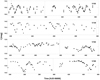 |
Fig. 9. I-band light curves of TTSs in our sample. The top panel shows a WTT displaying periodic brightness variations with similar amplitudes. The second panel shows a T Tauri star with a periodic variation together with multiple extinction events where magnitude fades significantly than its median value. The bottom two panels display CTTSs with different variability signatures (see text for details). |
The amplitudes in the VI filters are shown in Fig. 10 for all variable sources. WTTSs have amplitudes smaller than 0.7 mag while CTTSs exhibit large magnitude fluctuations up to 2.5 mag. Four stars exhibit variability amplitudes significantly larger in the I band than in the V band. These cases exhibit lower quality V-band light curves, which prevents an accurate determination of their luminosity maxima and minima. The colors of variability in all stars are also shown in the right panel of Fig. 10. The variation in the luminosity and colors displays a range of slopes attributed to different cause of variability. Variables display redder colors at fainter epochs when the variability is driven by spot modulation. The variability amplitudes increase towards shorter wavelengths more steeply when the light curves are dominated by accretion spots than in the case of cold spot modulation (Vrba et al. 1993). When the variability is driven by occultations due to opaque transiting material, little or no color variations are seen. The redder colors at fainter states are also observed in case of variability due to circumstellar extinction (Venuti et al. 2015). In Fig. 10, high-amplitude CTTSs display bluer colors than the smaller amplitude WTTSs. Most of the WTTSs stars show flatter slopes with little brightness variations, while a few CTTSs also occupy the region towards high luminosity with smaller color variations. The MS and field stars occupy a distinct region of the diagram with respect to the TTSs in our sample, and show very small variations in their amplitudes and colors.
 |
Fig. 10. Left panel: variation in V- and I-band amplitudes for all variables. Right panel: variability in the amplitude-color plane plotted in the CMD. Variation along I-mag is the difference between maximum and minimum, while (V − I) represents the range of the color curve. The color bar shows the ranges of I-band magnitudes. |
5.2. Bursters and faders
In PMS stars, an increase in accretion rate from the circumstellar disk onto the star can give rise to a significant burst in magnitude that lasts from hours to days (Cody & Hillenbrand 2018). Similarly, short-duration brightening events with typical variation of a few tenths of a magnitude can also be seen that last typically up to a few hours. As in case of prototype AA Tau, repetitive fading of magnitudes for PMS stars occurred due to circumstellar extinction. Findeisen et al. (2013) investigated bursters and faders with multiyear R-band time-series data from Palomar Transient Factory in the North America and Pelican Nebulae. Six of these stars (2 bursters and 4 faders) are found to be in common with our catalog. V195 was a fader around mid-2011 in Findeisen et al. (2013), while it shows a distinct brightening event lasting over 50 days at the end of 2012 in our photometry. Another fader, V182, shows a brightening event in November 2012, while V180 shows multiple extinction events as large as 2 mag. One burster, V121, in common with Findeisen et al. (2013) also displays periodic variations in this work. While typical short-term, discrete bursts that occur within days are missed in our photometry, some PMS variables do show significant brightening within ten days. For a simple quantitative measure, we define a burst as a change in brightness of more than 75% of total amplitude within 10 days and that occurs in the epochs that are brighter than the median magnitude of the light curve. Only 12 CTTSs display these possible bursting events in the light curves. Individual fading or brightening and bursting events are commented in Table 4, but we do not expect to observe any short-duration bursting events that only last one day, due to the limited number of observations per night.
5.3. Spectral energy distributions
The SEDs for the candidate PMS variables are constructed using the multiband photometric data compiled from the literature, as discussed in Sect. 2. Optical BVRI mean magnitudes and random-epoch infrared magnitudes are converted into millijansky fluxes to construct the observed SEDs. To infer the physical properties of these PMS stars, models of Robitaille et al. (2006, 2007) are fitted to the observed SEDs. The photometric uncertainties in the single-epoch infrared magnitudes are typically underestimated; therefore, a conservative estimate of uncertainties in the fluxes is adopted by adding a 10% error in the quadrature to the flux errors derived from the uncertainties in infrared magnitudes. Since the amplitudes in infrared are typically smaller, these adopted uncertainties are reasonable to account for the magnitude variation within a random-epoch. We emphasize that the SEDs generated from the radiative transfer models are subject to degeneracy as different combinations of parameters may result in a similar fit to the observed SEDs (Robitaille et al. 2007). This degeneracy could be remedied with spatially resolved observations at a range of wavelengths.
In order to fit SED models to the observed fluxes, the mean distance to the cluster is adopted for all PMS variables. The extinction is allowed to vary from zero reddening to a maximum AV of 10 mag for SED fitting. The range of AV is derived from the NIR CCD, as discussed previously. An upper limit of 24 μm is imposed while fitting SEDs, although 70 μm flux is also available for a small sample of stars. The physical parameters of PMS stars cannot be determined precisely if the number and range of wavelengths is small (Robitaille et al. 2007). However, SED fits can still be used to constrain certain physical parameters depending on the availability of photometric data and a reasonable range of physical parameters can be interpreted. Therefore, SED models are fitted only if there are at least ten flux measurements for a given PMS star, and we select only those models for which,  , where N is the number of data points. Figure 11 shows the SED fits of two variables in our sample. To estimate the physical parameters of the PMS stars, the mean values are estimated by weighted e(−χ2/2) of the 100 best-fit models that satisfy the χ2 condition, and the standard deviation is adopted as their associated uncertainties.
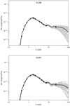 |
Fig. 11. Spectral energy distributions of two PMS variables. The black line shows the best-fit model, while the gray lines display the top 100 models that satisfy the criterion |

The typical ranges of mass and age estimates from the SED fitting are consistent with those derived from the isochrone fitting, but the individual estimates may differ between the two approaches. A median value of mass and age from SED fitting is found to be ∼1.1 M⊙ and ∼2 Myr, typically higher than isochrone-based estimates. No mass-dependent trend is seen in the age estimates, but the isochrone-based mass and age estimates could be systematically smaller for low-mass stars (Hillenbrand et al. 2008; Herczeg & Hillenbrand 2015; Pecaut & Mamajek 2016). The physical parameters obtained from the SED fits are listed in Table 5 for the PMS stars for a comparison. Furthermore, the luminosity and temperature estimates from the SED fitting are compared with the values provided in the Gaia catalog. While the luminosity values for common stars correlate well, the temperatures are consistent within their uncertainties only in the 3000−5000 K range. We also investigate possible correlations of variability periods and amplitudes with the physical parameters for PMS stars. No significant correlation is seen between the periods or amplitudes and the mass and age estimates for PMS stars. Venuti et al. (2015) observed an anticorrelation between observed variability amplitudes in u and r band, with stellar mass for WTTSs suggesting a uniform distribution of spots in more massive PMS stars. However, the limited sample of WTTSs in our sample preclude us from a detailed statistical analysis.
Physical parameters of PMS stars based on SED fitting.
6. Discussion and conclusions
We presented a catalog of optical time-series photometry of young stellar objects in the Pelican Nebula (IC 5070) star-forming region. Our data provide a significant increase in the number of pre-main-sequence variables in this region with multiband year-long optical photometry. Of the 95 variables in the targeted region, 67 objects are pre-main-sequence stars classified based on the multiband CMDs and CCDs. The five-parameter solutions from the recent Gaia data release are used to confirm the association of variables with the IC 5070 region using accurate proper motions and parallaxes. While the optical data are limited to three epochs per night at most, a total of more than 250 epochs in each VRI band allow us to further identify WTT and CTT candidates based on their light curve structure. Nearly 70% of PMS stars display photometric variations similar to CTTSs and 30% display strong periodic variations similar to WTTSs. Several CTTSs show significant extinction events and a few also exhibit the periodic variations. The amplitude variations for WTTSs are smaller than 0.4 mag, whereas the average amplitude variations for CTTSs are of 1 mag in V band. CTTSs also display several fading and brightening events as large as 2.5 mag in I band. The catalog includes probable long-period variables displaying long-lasting (>50 days) brightening events. CTTSs display typical magnitude fluctuations of up to three times the maximum variation seen in WTTSs in our sample.
Figure 12 shows the spatial distribution of candidate T Tauri stars. All variables are distributed throughout the targeted field and no obvious clustering is seen for T Tauri stars. Most of the PMS variables have subsolar masses and a median age of 2 Myr based on the isochrone fitting to optical CMDs. The individual mass and age estimates may differ between the isochrone-based estimates and SED fitting tools, but the typical ranges of these physical parameters are consistent between the two approaches. We do not find any evidence of a correlation between amplitude and physical parameters. While this work provided a catalog of variable sources, a detailed investigation into all pre-main-sequence populations and individual variable objects may be the subject of a future study.
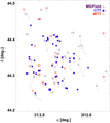 |
Fig. 12. Spatial distribution for different classes of variables along with their position 104 years ago indicated by the gray arrow. |
Variability studies of pre-main-sequence stars at shorter wavelengths can provide an insight into different physical properties of accreting and non-accreting young stellar objects. The candidate accreting CTTSs in our analysis display significantly higher variability than the disk-free WTTSs. The combined variations in the luminosity and colors for pre-main-sequence stars can be traced back to the root cause of their different variability signatures: accretion, circumstellar extinction, or spot-modulations. Short-cadence time-series photometry and spectroscopic follow-up is necessary to confirm the classification of T Tauri variables, which would in turn allow a more detailed investigation into the root cause of variability for the pre-main-sequence stars presented in this analysis.
Acknowledgments
We thank the anonymous referee for the detailed and useful comments that improved the quality of the paper. AB acknowledges research grant #11850410434 awarded by the National Natural Science Foundation of China through a Research Fund for International Young Scientists, and China Post-doctoral General Grant. NP acknowledges the financial support from the Department of Science and Technology, INDIA, through INSPIRE faculty award DST/IFA12/PH-36. HPS thanks the Council of Scientific & Industrial Research, India, for grant #03(1428)/18/EMR-II. We also thank Dr. Chow-Choong Ngeow for providing the standard transformation equations, and Dr. Tapas Baug for sharing his calibration and plotting routines. This research was support by the Munich Institute for Astro- and Particle Physics (MIAPP) of the DFG cluster of excellence “Origin and Structure of the Universe.” This publication makes use of data from the Two Micron All Sky Survey (a joint project of the University of Massachusetts and the Infrared Processing and Analysis Center/California Institute of Technology, funded by the National Aeronautics and Space Administration and the National Science Foundation), and archival data obtained with the Spitzer Space Telescope and Wide Infrared Survey Explorer (operated by the Jet Propulsion Laboratory, California Institute of Technology, under contract with the NASA.
References
- Alencar, S. H. P., Teixeira, P. S., Guimarães, M. M., et al. 2010, A&A, 519, A88 [NASA ADS] [CrossRef] [EDP Sciences] [Google Scholar]
- Ansdell, M., Gaidos, E., Rappaport, S. A., et al. 2016, ApJ, 816, 69 [NASA ADS] [CrossRef] [Google Scholar]
- Bailer-Jones, C. A. L., Rybizki, J., Fouesneau, M., Mantelet, G., & Andrae, R. 2018, AJ, 156, 58 [NASA ADS] [CrossRef] [Google Scholar]
- Bally, J., Ginsburg, A., Probst, R., et al. 2014, AJ, 148, 120 [NASA ADS] [CrossRef] [Google Scholar]
- Baraffe, I., Chabrier, G., & Gallardo, J. 2009, ApJ, 702, L27 [NASA ADS] [CrossRef] [Google Scholar]
- Baraffe, I., Vorobyov, E., & Chabrier, G. 2012, ApJ, 756, 118 [NASA ADS] [CrossRef] [Google Scholar]
- Bertout, C. 1989, ARA&A, 27, 351 [NASA ADS] [CrossRef] [Google Scholar]
- Bessell, M. S., & Brett, J. M. 1988, PASP, 100, 1134 [NASA ADS] [CrossRef] [Google Scholar]
- Bouvier, J., Cabrit, S., Fernandez, M., Martin, E. L., & Matthews, J. M. 1993, A&A, 272, 176 [NASA ADS] [Google Scholar]
- Bouvier, J., Forestini, M., & Allain, S. 1997, A&A, 326, 1023 [NASA ADS] [Google Scholar]
- Bressan, A., Marigo, P., Girardi, L., et al. 2012, MNRAS, 427, 127 [NASA ADS] [CrossRef] [Google Scholar]
- Cambrésy, L., Beichman, C. A., Jarrett, T. H., & Cutri, R. M. 2002, AJ, 123, 2559 [NASA ADS] [CrossRef] [Google Scholar]
- Cody, A. M., & Hillenbrand, L. A. 2018, AJ, 156, 71 [NASA ADS] [CrossRef] [Google Scholar]
- Cody, A. M., Stauffer, J., Baglin, A., et al. 2014, AJ, 147, 82 [NASA ADS] [CrossRef] [Google Scholar]
- Cohen, J. G., Frogel, J. A., Persson, S. E., & Elias, J. H. 1981, ApJ, 249, 481 [NASA ADS] [CrossRef] [Google Scholar]
- Cutri, R. M., Skrutskie, M. F., van Dyk, S., et al. 2003, The IRSA 2MASS All-Sky Point Source Catalog, NASA/IPAC Infrared Science Archive [Google Scholar]
- David, T. J., Hillenbrand, L. A., Gillen, E., et al. 2019, ApJ, 872, 161 [NASA ADS] [CrossRef] [Google Scholar]
- Eyer, L., & Mowlavi, N. 2008, J. Phys. Conf. Ser., 118, 012010 [NASA ADS] [CrossRef] [Google Scholar]
- Fernandes, R. B., Long, Z. C., Pikhartova, M., et al. 2018, ApJ, 856, 103 [NASA ADS] [CrossRef] [Google Scholar]
- Findeisen, K., Hillenbrand, L., Ofek, E., et al. 2013, ApJ, 768, 93 [NASA ADS] [CrossRef] [Google Scholar]
- Froebrich, D., Scholz, A., Campbell-White, J., et al. 2018, Res. Notes Am. Astron. Soc., 2, 61 [CrossRef] [Google Scholar]
- Gaia Collaboration (Brown, A. G. A., et al.) 2018a, A&A, 616, A1 [NASA ADS] [CrossRef] [EDP Sciences] [Google Scholar]
- Gaia Collaboration 2018b, VizieR Online Data Catalog: I/345 [Google Scholar]
- Gillen, E., Aigrain, S., Terquem, C., et al. 2017, A&A, 599, A27 [NASA ADS] [CrossRef] [EDP Sciences] [Google Scholar]
- Girardi, L., Bertelli, G., Bressan, A., et al. 2002, A&A, 391, 195 [NASA ADS] [CrossRef] [EDP Sciences] [Google Scholar]
- Grankin, K. N., Bouvier, J., Herbst, W., & Melnikov, S. Y. 2008, A&A, 479, 827 [NASA ADS] [CrossRef] [EDP Sciences] [Google Scholar]
- Guieu, S., Rebull, L. M., Stauffer, J. R., et al. 2009, ApJ, 697, 787 [NASA ADS] [CrossRef] [Google Scholar]
- Guo, Z., Herczeg, G. J., Jose, J., et al. 2018, ApJ, 852, 56 [NASA ADS] [CrossRef] [Google Scholar]
- Henden, A. A., Templeton, M., Terrell, D., et al. 2016, VizieR Online Data Catalog: II/336 [Google Scholar]
- Herbig, G. H. 1962, Adv. Astron. Astrophys., 1, 47 [NASA ADS] [CrossRef] [Google Scholar]
- Herbig, G. H. 1977, ApJ, 214, 747 [NASA ADS] [CrossRef] [Google Scholar]
- Herbst, W., Herbst, D. K., Grossman, E. J., & Weinstein, D. 1994, AJ, 108, 1906 [NASA ADS] [CrossRef] [Google Scholar]
- Herbst, W., Eisloffel, J., Mundt, R., & Scholz, A. 2007, in Protostars and Planets V, eds. B. Reipurth, D. Jewitt, & K. Keil (Tucson: University of Arizona Press), 297 [Google Scholar]
- Herczeg, G. J., & Hillenbrand, L. A. 2014, ApJ, 786, 97 [NASA ADS] [CrossRef] [Google Scholar]
- Herczeg, G. J., & Hillenbrand, L. A. 2015, ApJ, 808, 23 [Google Scholar]
- Hillenbrand, L. A., Carpenter, J. M., Kim, J. S., et al. 2008, ApJ, 677, 630 [Google Scholar]
- Ibryamov, S., Semkov, E., Milanov, T., & Peneva, S. 2018, Res. Astron. Astrophys., 18, 137 [NASA ADS] [CrossRef] [Google Scholar]
- Ikeda, H., Sugitani, K., Watanabe, M., et al. 2008, AJ, 135, 2323 [NASA ADS] [CrossRef] [Google Scholar]
- Joy, A. H. 1945, ApJ, 102, 168 [NASA ADS] [CrossRef] [Google Scholar]
- Kóspál, Á., Ábrahám, P., Acosta-Pulido, J. A., et al. 2011, A&A, 527, A133 [NASA ADS] [CrossRef] [EDP Sciences] [Google Scholar]
- Landolt, A. U. 2009, AJ, 137, 4186 [NASA ADS] [CrossRef] [Google Scholar]
- Lata, S., Pandey, A. K., Panwar, N., et al. 2016, MNRAS, 456, 2505 [NASA ADS] [CrossRef] [Google Scholar]
- Laugalys, V., Straižys, V., Vrba, F. J., et al. 2007, Balt. Astron., 16, 349 [NASA ADS] [Google Scholar]
- Lomb, N. R. 1976, Ap&SS, 39, 447 [NASA ADS] [CrossRef] [Google Scholar]
- Lucas, P. W., Hoare, M. G., Longmore, A., et al. 2008, MNRAS, 391, 136 [NASA ADS] [CrossRef] [Google Scholar]
- Luri, X., Brown, A. G. A., Sarro, L. M., et al. 2018, A&A, 616, A9 [NASA ADS] [CrossRef] [EDP Sciences] [Google Scholar]
- Messina, S., Parihar, P., & Distefano, E. 2017, MNRAS, 468, 931 [NASA ADS] [CrossRef] [Google Scholar]
- Meyer, M. R., Calvet, N., & Hillenbrand, L. A. 1997, AJ, 114, 288 [NASA ADS] [CrossRef] [Google Scholar]
- Ogura, K., Sugitani, K., & Pickles, A. 2002, AJ, 123, 2597 [NASA ADS] [CrossRef] [Google Scholar]
- Panwar, N., Chen, W. P., Pandey, A. K., et al. 2014, MNRAS, 443, 1614 [NASA ADS] [CrossRef] [Google Scholar]
- Pecaut, M. J., & Mamajek, E. E. 2016, MNRAS, 461, 794 [NASA ADS] [CrossRef] [Google Scholar]
- Poljančić, B. I., Jurdana-Šepić, R., Semkov, E. H., et al. 2014, A&A, 568, A49 [NASA ADS] [CrossRef] [EDP Sciences] [Google Scholar]
- Rebull, L. M., Guieu, S., Stauffer, J. R., et al. 2011, ApJS, 193, 25 [NASA ADS] [CrossRef] [Google Scholar]
- Reipurth, B., & Schneider, N. 2008, in Star Formation and Young Clusters in Cygnus, ed. B. Reipurth, 36 [Google Scholar]
- Robitaille, T. P., Whitney, B. A., Indebetouw, R., Wood, K., & Denzmore, P. 2006, ApJS, 167, 256 [NASA ADS] [CrossRef] [Google Scholar]
- Robitaille, T. P., Whitney, B. A., Indebetouw, R., & Wood, K. 2007, ApJS, 169, 328 [NASA ADS] [CrossRef] [Google Scholar]
- Rodriguez, J. E., Ansdell, M., Oelkers, R. J., et al. 2017, ApJ, 848, 97 [NASA ADS] [CrossRef] [Google Scholar]
- Scargle, J. D. 1982, ApJ, 263, 835 [NASA ADS] [CrossRef] [Google Scholar]
- Schwarzenberg-Czerny, A. 1989, MNRAS, 241, 153 [NASA ADS] [CrossRef] [Google Scholar]
- Semkov, E. H. 2011, Bulg. Astron. J., 15, 65 [Google Scholar]
- Siess, L., Dufour, E., & Forestini, M. 2000, A&A, 358, 593 [Google Scholar]
- Soderblom, D. R., Hillenbrand, L. A., Jeffries, R. D., Mamajek, E. E., & Naylor, T. 2014, Protostars and Planets VI, 219 [Google Scholar]
- Stassun, K. G., Feiden, G. A., & Torres, G. 2014, New Astron., 60, 1 [CrossRef] [Google Scholar]
- Stellingwerf, R. F. 1978, ApJ, 224, 953 [NASA ADS] [CrossRef] [Google Scholar]
- Stelzer, B. 2015, Astron. Nachr., 336, 493 [NASA ADS] [CrossRef] [Google Scholar]
- Stetson, P. B. 1987, PASP, 99, 191 [NASA ADS] [CrossRef] [Google Scholar]
- Stetson, P. B. 1993, in IAU Colloq. 136: Stellar Photometry – Current Techniques and Future Developments, eds. C. J. Butler, & I. Elliott, 136, 291 [NASA ADS] [Google Scholar]
- Stetson, P. B. 1996, PASP, 108, 851 [NASA ADS] [CrossRef] [Google Scholar]
- Venuti, L., Bouvier, J., Irwin, J., et al. 2015, A&A, 581, A66 [NASA ADS] [CrossRef] [EDP Sciences] [Google Scholar]
- Vrba, F. J., Chugainov, P. F., Weaver, W. B., & Stauffer, J. S. 1993, AJ, 106, 1608 [NASA ADS] [CrossRef] [Google Scholar]
- Zhang, S., Xu, Y., & Yang, J. 2014, AJ, 147, 46 [NASA ADS] [CrossRef] [Google Scholar]
Appendix A: Multiband light curves
The light curves of pre-main-sequence variable stars observed in all three bands (VRI) are shown in Fig. A.1. R-band light curves are shown in the middle (red) of each panel. Light curves in V/I bands are displayed above and below (blue and violet, respectively) the R band, and are offset by R-band amplitude for visualization purposes. The star ID and periods are given at the top of each panel. In the case of time light curves, the x-axis is offset by HJD–56000, while the vertical dashed line separates the observations in two different seasons. All light curves are normalized with zero-mean for a relative comparison and plotting purposes.
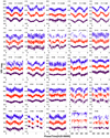 |
Fig. A.1. Phase (or time) light curves of variable stars. |
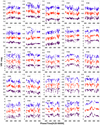 |
Fig. A.1. continued. |
All Tables
All Figures
|
Fig. 1. Color composite image of the young star-forming region towards Pelican Nebula obtained using the VRI-band images. The cyan circles represent the location of the variable stars. |
| In the text | |
|
Fig. 2. Top panel: photometric precision of our observations in I band as a function of instrumental magnitudes. Middle panel: root mean square (rms) scatter in I band as a function of instrumental magnitudes. Red circles denote the selected candidate variables in the top and middle panels. Bottom panel: Stetson’s J-index for all sources in our field as a function of instrumental I-band magnitudes. Red circles and triangles represent the variables with light curves available in RI and VI bands. |
| In the text | |
|
Fig. 3. Representative I-band light curves of periodic (top) and nonperiodic variables (bottom) with varying light curve quality. The magnitudes are normalized with respect to the zero-mean. Star ID, period, and mean magnitude are also provided in each panel. The vertical dashed line in the bottom panels separates the observations into two different seasons that are offset for visualization purposes. |
| In the text | |
|
Fig. 4. Scatterplot of variable sources in the proper motion plane. Histograms for proper motions along right ascension and declination are also shown. The center of the circles is at the peak values of proper motions from the Gaussian distribution fits to the histograms. The inner and outer radius is of 2 and 4 mas per year, respectively. Filled circles denote kinematically selected members. Open triangles represent 3σ (∼2 mas per year) outliers from the mean of the Gaussian distribution fits to the histograms of the proper motions. Filled triangles display variables for which the proper motions are consistent with the mean value given their 3σ uncertainties. The bin size used in the histograms and the number of stars shown are indicated at the top. |
| In the text | |
|
Fig. 5. Top panel: scatterplot of parallaxes against the proper motions along right ascension and declination. The symbols are the same as in Fig. 4. Bottom panel: histogram of parallaxes for variable sources from the Gaia DR2. The bin size used in the histogram and the number of stars shown in the plots are indicated at the top. |
| In the text | |
|
Fig. 6. Near-infrared CCD for all variables. The solid curve and dotted curve represent the sequence of dwarf and giants from Bessell & Brett (1988). The locus of CTT stars is shown as long-dashed lines (Meyer et al. 1997), while the dot-dashed lines represent the reddening vectors (Cohen et al. 1981). Diamonds and open triangles represent the kinematic members and outliers, respectively. The solid arrow indicates reddening vector corresponding to AV = 5 mag. Each star is numbered with the last two digits of the Star ID from Table 2. |
| In the text | |
|
Fig. 7. Apparent optical V/V − I CMD for the variable candidates. The dashed curve shows the isochrones for PMS stars with different ages from Siess et al. (2000), while the solid curve is the ZAMS by Girardi et al. (2002). The dotted curves display the evolutionary tracks of PMS stars with different stellar masses. The isochrones and the evolutionary tracks are offset with respect to the average distance (857.5 pc) and extinction (AV = 1.9 mag). The color bar represents the 2MASS (H − K) color. Open triangles represent the kinematic outliers. The arrow indicates the direction of the reddening vector corresponding to AV = 5 mag. |
| In the text | |
|
Fig. 8. K/I − K CMD. The stars are numbered with the last two digits of their Star ID from Table 2. The color bar represents the age determined from the isochrone fitting. Open triangles represent the kinematic outliers. The arrow indicates the reddening vector corresponding to AV = 5 mag. The increase in symbol size represents the increase in mass obtained from the evolutionary tracks. |
| In the text | |
|
Fig. 9. I-band light curves of TTSs in our sample. The top panel shows a WTT displaying periodic brightness variations with similar amplitudes. The second panel shows a T Tauri star with a periodic variation together with multiple extinction events where magnitude fades significantly than its median value. The bottom two panels display CTTSs with different variability signatures (see text for details). |
| In the text | |
|
Fig. 10. Left panel: variation in V- and I-band amplitudes for all variables. Right panel: variability in the amplitude-color plane plotted in the CMD. Variation along I-mag is the difference between maximum and minimum, while (V − I) represents the range of the color curve. The color bar shows the ranges of I-band magnitudes. |
| In the text | |
|
Fig. 11. Spectral energy distributions of two PMS variables. The black line shows the best-fit model, while the gray lines display the top 100 models that satisfy the criterion |
| In the text | |
|
Fig. 12. Spatial distribution for different classes of variables along with their position 104 years ago indicated by the gray arrow. |
| In the text | |
|
Fig. A.1. Phase (or time) light curves of variable stars. |
| In the text | |
|
Fig. A.1. continued. |
| In the text | |
Current usage metrics show cumulative count of Article Views (full-text article views including HTML views, PDF and ePub downloads, according to the available data) and Abstracts Views on Vision4Press platform.
Data correspond to usage on the plateform after 2015. The current usage metrics is available 48-96 hours after online publication and is updated daily on week days.
Initial download of the metrics may take a while.