| Issue |
A&A
Volume 686, June 2024
|
|
|---|---|---|
| Article Number | A269 | |
| Number of page(s) | 9 | |
| Section | Catalogs and data | |
| DOI | https://doi.org/10.1051/0004-6361/202349114 | |
| Published online | 19 June 2024 | |
Young stellar objects from the LAMOST and ZTF surveys: Physical properties, classification, and light curve analysis
1
CAS Key Laboratory of Optical Astronomy, National Astronomical Observatories,
Beijing
100101, PR China
e-mail: This email address is being protected from spambots. You need JavaScript enabled to view it.
2
National Astronomical Observatories,
Beijing
100101, PR China
3
University of Chinese Academy of Sciences,
Beijing
100049, PR China
Received:
28
December
2023
Accepted:
14
March
2024
Abstract
Context. The study of young stellar objects (YSOs) not only enhances our understanding of star formation and stellar evolution, but also contributes to broader areas of astrophysics, including planetary science, galactic dynamics, and astrochemistry.
Aims. We aimed to comprehensively analyse 657 YSOs and provide their physical parameter measurements using data from Zwicky Transient Facility (ZTF) g- and r-band light curves and the Gaia, WISE, 2MASS, and LAMOST databases. Specifically, we sought to identify periodicity in the light curves and classify the YSOs based on the Q – M variability plane, which enabled us to quantify flux asymmetry and quasi-periodicity.
Methods. To achieve our objectives, we conducted a meticulous examination of the light curves obtained from the ZTF and estimated the physical parameters of the YSOs. These parameters were discerned by integrating stellar model atmosphere grids, photometric data, Gaia DR3 parallaxes, and pre-main-sequence evolutionary tracks. We employed the Q – M variability plane to classify the YSOs and determine the presence of periodic patterns. Additionally, we analysed the distribution of variability slope angles in the colour-magnitude diagram (CMD) to discern patterns associated with extinction-driven and accretion-related variability.
Results. Our analysis revealed significant findings regarding the variability patterns and physical characteristics of the YSOs. Among the 657 objects analysed, 37 exhibited periodic variability and 2 displayed multi-period behaviour. Furthermore, we identified distinct variability patterns, including quasi-periodic symmetry, quasi-periodic dipping, aperiodic dipping, bursting behaviour, stochastic variability, and long-timescale variations. Notably, the distribution of variability slope angles in the CMD varied between dippers and bursters, indicating different underlying variability drivers. Additionally, we observed that YSOs classified as classical T Tauri stars and weak-line T Tauri stars exhibited contrasting light curve characteristics, with Class II YSOs displaying asymmetry and Class III YSOs showing (quasi-)periodic variations. These findings underscore the importance of considering variability patterns when classifying and determining the nature of YSOs.
Key words: methods: data analysis / techniques: miscellaneous / catalogs / stars: pre-main sequence / stars: variables: general
The LAMOST spectra and full Tables 3 and 5 are available at the CDS via anonymous ftp to cdsarc.cds.unistra.fr (138.79.128.5) or via https://cdsarc.cds.unistra.fr/viz-bin/cat/J/A+A/686/A269
© The Authors 2024
 Open Access article, published by EDP Sciences, under the terms of the Creative Commons Attribution License (https://creativecommons.org/licenses/by/4.0), which permits unrestricted use, distribution, and reproduction in any medium, provided the original work is properly cited.
This article is published in open access under the Subscribe to Open model. This email address is being protected from spambots. You need JavaScript enabled to view it. to support open access publication.
1 Introduction
Variability has long been known to be a prevailing characteristic of young stellar objects (YSOs; Joy 1945). Different timescales related to YSO variability can reveal various phenomena that occur in the YSO inner disk system. These phenomena include mass accretion from the inner disk onto the star, magnetic activity (including energetic manifestations such as stellar flares and coronal mass ejections), and geometric effects such as rotational luminosity modulation from surface spots or obscuration by inner disk warps along the line of sight to the source (Bonito et al. 2023). Many surveys have reported YSO variability on both short (hours to days) and long timescales (months to years). The CoRoT (a CNES-led mission with ESA participation; Auvergne et al. 2009) and Kepler (Borucki et al. 2010) spacecraft investigated this variability with high-cadence observations from space, using a single broadband filter. They could only observe a limited number of star-forming regions (SFRs) along their orbits. Since the CoRoT and Kepler spacecrafts are no longer operational, the only space-based facility that could currently provide high-cadence observations of YSO variability is the Transiting Exoplanet Survey Satellite (TESS; Ricker et al. 2014). However, the TESS is less suitable for SFR studies due to its large pixel size, which makes it difficult to distinguish individual sources in potentially dense regions. Moreover, studies have demonstrated that adding colour information is helpful for a consistent physical explanation of the variability (e.g. Cody & Hillenbrand 2018). The Zwicky Transient Facility (ZTF; Bellm et al. 2018) employs a 47 deg2 wide field-of-view camera, scanning the northern sky at high cadence (≈2 days) to produce a comprehensive and multi-filter survey. This enables high-quality and reliable data products that can be used to study time-varying phenomena. Furthermore, archival data from ZTF will provide a pathway to the next-generation surveys, such as the Rubin Observatory Legacy Survey of Space and Time (LSST).
The diversity of light curve shapes is usually the result of different physical processes that affect the brightness of YSOs over time. Our light curve classification scheme follows the quasi-periodicity (Q) and flux asymmetry (M) statistics developed by Cody et al. (2014). They classified YSOs into different variability categories, including periodic, dipping, bursting, quasi-periodic, stochastic, and long-timescale. The morphology of light curves can reflect physical processes. One possible cause of periodic variability in YSOs is rotational modulation. Dipping YSOs are often surrounded by gas and dust disks that can produce eclipses or obscuration due to clumps or warps in the disk, or they have strong magnetic fields that induce changes in the scale height of the inner disk. By classifying light curves based on their shape and symmetry, we can infer the underlying mechanisms of variability and learn more about the properties of YSOs. Bursting YSOs are typically associated with accretion instabilities. For quasi-periodic YSOs, there are two possible explanations. One possibility is that they are a result of a combination of periodic variations, such as cool starspot modulation, and aperiodic changes on longer timescales, such as those arising from accretion processes. Another possibility is that the variability is caused by a single process that is not entirely stable from cycle to cycle. Examples of this phenomenon include stellar hot spots that change in brightness due to stochastic accretion flow. Stochastic YSOs may be affected by a combination of variable extinction and stochastic accretion, which can produce irregular and asymmetric light curves. The long-timescale variability observed in YSOs likely reflects disk dynamics beyond the inner edge.
In this work, our primary goal is to analyse the physical properties of a sample of 657 YSOs. This paper is organized as follows: Sect. 2 provides a brief description of the sample selection and data. In Sects. 3 and 4, we describe the classification and stellar properties of the sample, respectively. Section 5 discusses the light curve analysis, and Sect. 6 provides the discussion and summary.
2 Data
Our initial sample consisted of 833 YSO candidates from previous work (Zhang et al. 2023, hereafter Paper I). In Paper I, we applied the self-paced ensemble (SPE) algorithm to classify different transients and variables, and then obtained 833 YSO candidates cross-matched with all stars ever observed with the Large Sky Area Multi-Object Fiber Spectroscopic Telescope (LAMOST; Wang et al. 1996; Cui et al. 2012). Three sources in the sample were excluded: two were identified as carbon stars according to LAMOST spectra, and the third was identified as a white dwarf.
To describe different variability classes of YSOs and provide a better understanding of the nature of the variability, we analysed the light curve data from the fourth public ZTF data release (ZTF DR4), which covers more than two years of observations, from 28 March 2018 to 6 June 2020. The ZTF light curves have a median cadence of about one day. The observations were usually taken every night, with some gaps of about 30 days due to seasons and some shorter gaps due to bad weather. We excluded observations that were affected by clouds or the Moon (these have catflag = 32 768). We also excluded the observations from MJD 58448 to 58456 because they are part of the ZTF high-cadence experiments that have poor photometry due to bad weather, which could affect the period search and classification of YSOs.
Our analysis mainly used data from the ZTF’s g band and r band, as the long-term i-band survey mostly focuses on fields with high galactic latitude. We only analysed objects that have an average g ≤ 20.8 mag or an average r ≤ 20.6 mag throughout the time series, and then removed any potential outliers that deviate from the median magnitude of the light curve by more than 5σ.
We also required at least 30 observations in both the g band and r band. A summary of the cuts applied to our initial sample and its subsequent refinement is presented in Table 1. In the end, our sample consisted of 657 YSOs; Figs. 1 and 2 show them in Galactic coordinates. Based on the currently identified SFRs within the Gould Belt, we determined that some of the YSOs are roughly distributed across the SFRs, as illustrated in Table 2. The distances of these sources are consistent with the known SFRs.
Remaining sample size following the application of the selection criteria.
Some SFRs related to YSOs within the Gould Belt.
3 YSO classification
At infrared wavelengths, YSOs are easier to detect because they show infrared excess and are less affected by visual extinction. With the help of infrared information, we can distinguish different evolutionary stages of YSOs. Lada (1987) and Allen et al. (2004) used classes from 0 to III to label these stages based on the slope of the spectral energy distribution (SED) in the infrared bands, which is measured by its spectral index. The spectral index is typically measured between 2 and 24–25 microns, and infrared excess comes from radiation from the disk and envelope for the youngest Class 0 and I sources. Many previous works performed classifications based mainly on Spitzer photometry (Dunham et al. 2015; Luhman et al. 2016).
Instead of computing the spectral index, we relied on machine learning to determine the classification of our YSO sample and to train a simple artificial neural network (ANN) classifier (shown in Fig. 3). The ANN structure consists of one input layer, two hidden layers (50 nodes for the first hidden layer and 10 nodes for the second hidden layer), and one output layer. It uses sigmoid activation for hidden layers and probabilistic Softmax activation for the output layer. The training sample is from the Cornu & Montillaud (2021) catalogue and contains 1306 Class II and 5316 Class III YSOs. Similar to Cornu & Montillaud (2021), the ANN model takes as input both magnitudes and their uncertainties from the Pan-STARRS DR1, the Two Micron All Sky Survey (2MASS), and the Wide-field Infrared Survey Explorer (WISE) surveys. The input includes gmag, rmag, imag, zmag, ymag, Jmag, Hmag, Kmag, W1mag, and W2mag and their uncertainties. The model achieves 96.4% accuracy on a test set comprising 30% of the total labelled dataset. When applying the model to a sample of 571 YSOs (those without missing values out of the 657 YSOs in our initial sample), we find that most of them fall into the first category, with only 23 targets falling into the second category. This may be due to selection effects impacting the collection of the unlabelled dataset. It should be noted that we excluded targets with missing measurements. We did not consider Class 0 or Class I YSOs because Class 0 YSOs are not observed and Class I YSOs are unlikely to be detected at optical wavelengths.
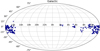 |
Fig. 1 Footprint of the 657 YSOs in Galactic coordinates. |
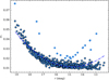 |
Fig. 2 Average r-band photometric error as a function of the average r magnitude. The variable stars in our final selection are represented as circles with dark blue outlines, and the light blue dots are anomalies that deviate from the main trend, denoted by the dash-dotted curve. These anomalies may experience a sudden fading or brightening event. |
4 Physical properties
This section is dedicated to establishing the stellar parameters, encompassing distances, extinctions, effective temperatures, stellar luminosities, masses, and ages of our YSOs. These parameters were derived through the integration of stellar model atmosphere grids, photometric data, Gaia DR3 parallaxes, and pre-main-sequence (PMS) evolutionary tracks.
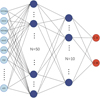 |
Fig. 3 ANN model used for YSO classification. Light blue dots represent input nodes for each required feature. Dark blue dots denote hidden neurons with sigmoid activation, while red dots represent output neurons with probabilistic Softmax activation. Black lines illustrate the connecting weights. Not all hidden neurons and weights are shown, for readability purposes. CII denotes a source classified as Class II and CIII a source classified as Class III. σ denotes the errors in different bands. |
4.1 Distance and extinction
For the estimation of extinction and stellar luminosity, accurate distance measurements are paramount. Gaia Data Release 3 (DR3) has furnished us with such measurements, including detailed information on the parallax and associated uncertainties of each celestial object. Leveraging these data, we derived distance estimates by inverting the parallaxes provided for YSOs.
Extinction primarily comprises two components: interstellar extinction and circumstellar extinction. The determination of extinction is crucial for correcting observed photometry via de-reddening before analysis. If the extinction is non-negligible, the true SED can deviate significantly from the observed one. Failing to properly correct for reddening can lead to erroneous estimations of any physical properties derived from the SED. We obtained the optimal extinction using the SED fitting method supported by the online tool Virtual Observatory SED Analyzer (VOSA)1. VOS A queries multiple photometric catalogues accessible through Virtual Observatory services, retrieves theoretical models, and computes their synthetic photometry. It then conducts a statistical test to identify the model that most accurately replicates the observed data. Given a range of values for Av, the model fits (chi2) the model physical parameters and the value for Av. Here, the Av range was set to 0−5 mag, from which we obtained the estimations of Av and their uncertainties.
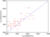 |
Fig. 4 Teff from existing literature vs. the estimated Teff. |
4.2 Effective temperature and luminosity
This section explains how stellar physical properties were derived. We queried the observed photometric data from Gaia DR3 (Riello et al. 2021), WISE (Wright et al. 2010), and 2MASS (Skrutskie et al. 2006) through VOSA for our sample. Using the obtained Av and distances with their uncertainties, we predicted the Teff and log L of each object in our sample using the MADYS tool (Squicciarini & Bonavita 2022). Specifically, the observed SED for each object was compared with synthetic photometry derived from theoretical modelling via a chi-square test. To derive parameter uncertainties, we generated 100 virtual SEDs by introducing Gaussian random noise for each object. Subsequently, statistical analysis was performed on the distribution of the obtained values for each parameter. The standard deviation of this distribution was then reported as the uncertainty associated with the respective parameter.
As illustrated in Fig. 4, we benchmarked the estimated Teff against existing literature values by employing queries in the SIMBAD astronomical database which provides basic data, cross-identifications, bibliographies and measurements for astronomical objects outside the Solar system. The comparison reveals that our results are largely in agreement with those documented in the literature, underscoring the reliability and accuracy of our methodology and the data sources employed.
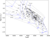 |
Fig. 5 HRD of the our sample overlaid with isochrones (dashed grey lines) and mass tracks (dashed blue lines) with solar metallicity from the PARSEC stellar model. |
4.3 Age and mass determination
By comparing the positions of sources on the Hertzsprung-Russell diagram (HRD), after correcting the distance and extinction, with theoretical grids from stellar evolution models, we estimated several astrophysical parameters, including mass and age. These parameters can be inferred by aligning the photometric data of celestial objects with the isochrone grids from the PARSEC stellar models (Bressan et al. 2012). Interpolating between the nearest points on the evolutionary tracks, we deduced the stellar masses and ages. The associated uncertainties in these estimates were primarily determined by the inaccuracies in the effective temperature (Teff) and stellar luminosity measurements. The tracks for stellar age and mass are illustrated in Fig. 5. Our analysis reveals that the majority of our sample falls within an age range of 0.1 to 6.5 Myr, with an average age of 3.5 Myr. Furthermore, over 90% of the stars in our sample have masses of less than 0.7 M⊙, with an average mass of 0.5 M⊙. The physical properties of the stars in our sample are comprehensively catalogued in Table 3. Given the use of the MADYS tool for estimating the ages and masses of YSOs, it is essential to acknowledge the inherent limitations associated with the isochronal fitting algorithm employed for age determination. Consequently, we would like to remind readers to exercise caution when using the age and mass estimations provided for these YSOs in our catalogue.
4.4 Accretion based on Hα emission
Of the 657 YSOs in our sample, 332 show Hα emission in the LAMOST spectra. PMS stars can be divided into classes based on the strength of the Hα emission line: classical Τ Tauri stars (CTTSs) and weak-line Τ Tauri stars (WTTSs). The main difference is that CTTSs have a disk of gas and dust around them and are actively accreting, while WTTSs have no disk or a very thin one and are not accreting.
We used the Hα equivalent width (EW(Hα)) to distinguish CTTSs from WTTSs. To estimate the uncertainty of the EW(Hα), we created multiple synthetic spectra by perturbing the observed flux values based on the measurement errors. We then examined the distribution of the EW(Hα) obtained from the Monte Carlo simulation with 1000 iterations and calculated the standard deviation of the distribution to represent the uncertainty. The cutoff value for EW(Hα) depends on the stellar spectral type. Fang et al. (2009) proposed that a source be classified as a CTTS if EW(Hα) ≥ 3 Å for K0-K3 stars, EW(Hα) ≥ 5 Å for K4 stars, EW(Hα) ≥ 7 Å for K5–K7 stars, Ew(Hα) ≥ 9 Å for M0–M1 stars, Ew(Hα) ≥ 11 Å for M2 stars, Ew(Hα) ≥ 15 Å for M3–M4 stars, EW(Hα) ≥ 18 Å for M5–M6 stars, and EW(Hα) ≥ 20 Å for M7–M8 stars. For this subsample of YSOs, 228 are classified as CTTSs and 45 as WTTSs.
Properties of our YSO sample.
4.5 Mass accretion rate
Another quantity, Hα (10%), was proposed by White & Basri (2003) as a way to distinguish between accreting and non-accreting objects. Hα (10%) is the full width of the line at 10% of the peak intensity, and they assumed that objects are accreting if Hα(10%) ≥270 km s−1, according to their measurements. In addition to indicating accretion, the Hα (10%) value can also provide a quantitative estimate of the mass accretion rate. Natta et al. (2004) derived the following correlation between Hα(10%) and the mass accretion rate, Ṁac:
 (1)
(1)
where Ṁac is in M⊙ yr−1 and Hα(10%) in km s−1.
We calculated the mass accretion rate and uncertainty of our sample and show the results in Table 3. Similar to the uncertainty of the calculation in EW(Hα), we also employed a Monte Carlo simulation with 1000 iterations to calculate the uncertainty of the mass accretion rate. We note that several of these targets are variable, and their variability can be related to the mass accretion rate, with Hα(10%) also being variable. Therefore, the mass accretion rate values inferred here are those observed at the epoch of the LAMOST observations.
5 Light curve analysis
Our analysis of the light curves presented in this section mainly relied on the r-band photometry because it has a higher quality and cadence than the g-band photometry. The g-band photometry was only used in some specific cases, such as for colour-magnitude diagram (CMD) analysis or if no significant period is found with r-band photometry.
5.1 Variability search
To measure the variability amplitude of objects in our working sample, we used the normalized peak-to-peak variability metric ν (Sokolovsky et al. 2017), which is defined as the ratio of the difference between the maximum and minimum magnitude measurements (mi) and the corresponding measurement uncertainties (σi). It is defined as follows:
 (2)
(2)
Hillenbrand et al. (2022) find that ν is well correlated with the standard deviation, with ν being about six times smaller. Before calculating ν, we applied a 5σ clip to all light curves to remove possible outliers, which is essential for the metric to be a reliable indicator of variability. We adopted the criterion of Hillenbrand et al. (2022) and classified an object as variable if its ν metric exceeds the 15th percentile of ν as a function of mean r magnitude, as shown in Fig. 6.
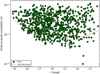 |
Fig. 6 Normalized peak-to-peak variability metric, ν, vs. the mean r magnitude for our sample. The dashed line marks the 15th percentile of ν, and the objects in green above it are considered variables. |
5.2 Period search
Since our ZTF data stream lasted for about 800 days, light curves with periods longer than 400 days only have at most one complete cycle in our analysis. To calculate the periodogram for each variable, we used the Lomb–Scargle periodogram (LSP) implementation in Astropy (VanderPlas & Ivezić 2015) and searched for periodic signals ranging from 0.5 days to 250 days. It is important to be aware of the failure modes of the periodogram approach when using LSP. These failure modes are caused by the aliasing effects that stem from the structure of the window function. Some aliases of the true frequency, rather than the true frequency itself, often correspond to the highest peak in the periodogram. For every object in our sample, when calculating the periodogram, we marked periods in the ranges 0.5–0.51, 0.98–1.02, 1.96–2.04, and 26–30 days to avoid the most common aliases pertaining to the solar and sidereal days and the lunar cycle (Rodriguez et al. 2017; Ansdell et al. 2018). Periodic signals that are not purely sinusoidal may have power at higher harmonics. Therefore, we also flagged periods that may be aliases with half or double multiples. If the dominant r-band period fails in the aforementioned alias checks, the dominant period was re-evaluated in the g-band.
We then calculated the false alarm probability (FAP) levels for 90%, 95%, and 99% confidence, and chose the period that corresponds to the highest power peak above the 99% confidence as significant. If there are no peaks that are more significant than the 99% confidence level, we used the period that corresponds to the maximum power of the periodogram. In the majority cases, we chose the peak with the maximum power as the real period, but sometimes we selected a peak with a slightly lower power because it explains the beat patterns corresponding to the approximately 1-day sampling interval better. Based on our visual inspection, we only checked the first four highest peaks for sources with more than four peaks in their periodograms. We marked the source as multi-periodic (MP) if there are more than two peaks with frequencies that are not aliases or beats of the selected real period.
5.3 Light curve classification
Our light curve classification scheme follows the quasi-periodicity (Q) and flux asymmetry (M) statistics first developed by Cody et al. (2014) and further refined by Cody et al. (2014):
 (3)
(3)
 (4)
(4)
We used the r-band light curve data to calculate the Q and M metrics for each object in most cases. For a few cases, we only determined the period for the g-band light curve, and used it to calculate these statistics as well. The classification boundaries based on Q and M are summarized in Table 4. Based on their locations in the Q–M plot and other visual criteria, the variables in our sample are grouped into seven categories, as shown in Fig. 7 and Table 5.
There are another two types of variables: long-timescale (L) variables, which have variability timescales of over 100 days, and MP variables, which have more than one period. We used linear least-squares fitting to detect a linear trend of rising or falling fluxes for L-type variables. Throughout our analysis, we considered a source to be robustly fit by a linear slope when FAPLin < 10−4. Although LSP can detect this linear trend, it can yield a too high variability amplitude if the variability is not genuinely periodic. Thus, linear least-squares fitting provides a better measure of variability for L-type YSOs. Figure 8 illustrates light curves for each category.
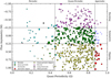 |
Fig. 7 Flux asymmetry vs quasi-periodicity of variables in our sample on the Q–M plot, with different colours for each light curve type. The point size shows the peak-to-peak variability metric, ν, scaled linearly. The Q–M classification is mostly accurate, with only a few sources needing manual adjustment. |
5.4 Colour-magnitude analysis
In order to investigate the physical drivers of the variability of YSOs, we compared the light curve morphology classes in terms of their variability in the CMD. The ZTF g-band and r-band observations were taken within a few hours up to a few days of each other, but they are not simultaneous. We trimmed the r-band light curve for each source into the corresponding g-band time span. For each g-band value that is paired with an r-band observation, linear interpolation was used to estimate g–r colours if the time interval of the paired g-band observations is less than 3 days. The errors of the interpolated g magnitudes and g–r colours were estimated using the Python package uncertainties (Lebigot 2010). A least-squares linear orthogonal fit to its CMD was performed using the Python package scipy.odr (Virtanen et al. 2020). After computing the best-fit slopes in g vs. g – r, we defined slope angles as the inverse tangent. The angles in degrees increase clockwise from 0° (corresponding to colour variability with no associated g-band variability) to 90° (colourless g-band variability). To compute errors on the best-fit angles, we used the PYSOVAR function fit_twocolor_odr (Günther et al. 2014). We note that slope angles with errors of less than 10 are significant. Similar to Poppenhaeger et al. (2015), we plotted the CMD slope angles of our sample against the CMD vector lengths that correspond to their flux asymmetry (M) classes, as shown in Fig. 9. We assessed the CMD slope angles in the context of standard reddening due to dust. The YSOs in our sample with time-variable CMD behaviour that is dominated by extinction effects have slope angles between 74.1° and 79.2°, which is consistent with Hillenbrand et al. (2022). In Fig. 9, it is clear that the majority of slopes are much shallower than what would be expected from purely reddening variations. The distribution of slope angles indicates that much of the observed variability is at least partially related to accretion effects, with some effects from extinction. The variables that have dips in flux are more common at the highest vector lengths and slope angles; the variables that have bursts in flux, on the other hand, are more common at the lowest vector lengths and slope angles. We also visually checked the bursters with slope angles greater than expectations from reddening variations. Some bursters lie at the boundary between the symmetric variables and bursters, and the angle errors of some are approximately 10°. So the distribution of CMD slope angles for dippers and bursters is very different, with dippers having slope angles that are closer to what we would expect from variability caused by extinction, and bursters having slope angles that are much flatter, which indicates variability related to accretion.
Light curve morphology classification based on the Q and M values.
Light curve classification of our sample according to the Q and M values.
5.5 Physical parameter distribution
Sections 4 and 5 describe how to calculate astronomical physical parameters and classify light curves. This section mainly discusses the distribution of astronomical physical parameters of different types of YSOs (Class II and Class III) and different light curve morphologies (see Figs. 10 and 11). As shown in Fig. 10, quasi-periodic symmetric and quasi-periodic dipping YSOs have similar physical parameters; aperiodic dipping YSOs have slightly higher luminosities and slightly higher effective temperatures; and dipper YSOs have a higher median effective temperature and higher luminosities than burster YSOs because dipper YSOs are more evolved and less obscured by their disks or envelopes than burster YSOs. There may be some exceptions or uncertainties depending on the individual properties and environments of each YSO. As indicated in Fig. 11, more evolved YSOs (Class III YSOs) have a higher mean effective temperature, an older age, and a higher mass, while Class II YSOs have a higher Ṁac with accretion-related variability drivers than Class III YSOs; both kinds of YSOs have comparable luminosities, which is consistent with the evolution of YSOs.
6 Discussion and summary
In this study we examined the YSO candidates identified in Paper I, providing analyses of their variability, physical properties, and classifications based on various criteria. Our primary findings are as follows:
- 1.
We conducted a search for periodicity in the light curves of all variable objects in our sample and classified them using the Q – M variability plane, to quantify flux asymmetry and quasi-periodicity in the light curves. Out of our 657 37 exhibit periodic variability, 2 display MP variability, 177 show quasi-periodic symmetric behaviour, 279 exhibit quasi-periodic dipping, 17 show aperiodic dipping, 111 demonstrate bursting behaviour, 24 display stochastic variability, and 8 exhibit long-timescale variability;
- 2.
The age mass, Teff, and log L of each object in the sample were estimated via a comparison with isochrone grids from the PARSEC stellar model. Most of our YSOs have ages ranging from 0.1 Myr to 6.5 Myr, with a mean age of 3.5 Myr. Additionally, more than 90% of the objects have masses of less than 0.7 M⊙, with a mean mass of 0.5 M⊙;
- 3.
We divided our subsample into classes: 228 are classified as CTTSs and 45 as WTTSs. Accretion based on Hα emission also provides us with a way to calculate the mass accretion rate;
- 4.
We examined the relationship between light curve morphology classes and variability patterns in CMDs to explore the possible causes of variability. Consistent with the findings of Hillenbrand et al. (2022), dippers and bursters exhibit different distributions of variability slope angles in CMDs, with dippers showing greater consistency with extinction-driven variability phenomena and bursters displaying much flatter slopes, which are indicative of accretion-related variability drivers;
- 5.
YSOs with different light curve classifications have distinct physical parameters (e.g. mass, Teff, and luminosity). Class II and III YSOs exhibit different physical parameters (e.g. mass, Teff, Ṁac, and age).
In our research, we employed the MADYS tool to predict the ages and masses of YSOs. This tool, which utilizes the algorithm of isochronal fitting for age determination, inherently faces the limitations associated with this methodology. Specifically, MADYS may not accurately distinguish between young PMS stars and more evolved stars that have departed from the main sequence. This ambiguity can lead to a range of possible solutions, especially when the age parameter is left unconstrained, as noted by Squicciarini & Bonavita (2022). Consequently, for very young stars, the ages reported by MADYS might not be reliable. Therefore, we advise readers to use the age and mass estimations for these YSOs in our catalogue with caution.
We present a comprehensive catalogue encompassing the physical parameters and light curve analyses of 657 YSOs meticulously observed by ZTF and LAMOSt. Employing deep learning techniques, we have succinctly classified YSOs into Class II and Class III based solely on photometric data. With the continual augmentation of Class 0, I, II, and III YSO samples, alongside the incorporation of infrared data, our forthcoming efforts are geared towards a more intricate classification of YSOs.
The proficiency of machine learning in adeptly classifying and identifying YSOs hinges upon the meticulous construction of robust models and the availability of adequately representative training samples. Ongoing and prospective survey initiatives, such as ZTF, LSST, and Euclid, are poised to afford us opportunities to unearth additional YSOs. In tandem with submillimeter spectroscopy, our ambition is to delve deeper into the outflow activities and molecular abundances intricately linked with YSOs.
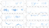 |
Fig. 8 Light curves for each category. |
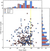 |
Fig. 9 Fitted CMD slope angle in degrees vs. Pythagorean vector length in magnitudes, sorted by flux asymmetry class. The majority of objects have slope angles much shallower than the expectations from reddening (shaded band), illustrating that the observed colour variability is dominated by accretion effects rather than by extinction effects. |
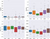 |
Fig. 10 Box plots of physical parameters for different YSOs with light curve classifications. |
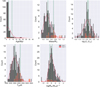 |
Fig. 11 Histograms of physical parameters for Class II and III YSOs. The x-axis shows the physical parameters. The y-axis shows the number of YSOs for a certain physical parameter. Histogram distributions of Class II and Class III YSOs are indicated in black and red, respectively. The dashed green line represents the average value line, and the solid red line represents the fitted kernel density estimation line. |
Acknowledgments
We extend our sincere gratitude for the referee’s meticulous review and invaluable feedback on our manuscript. His insightful comments and constructive criticisms have undoubtedly strengthened the quality and clarity of our work. This paper is funded by the National Natural Science Foundation of China under grants nos. 12203077, 12273076 and 12133001, the science research grants from the China Manned Space Project with Nos. CMS-CSST-2021-A04 and CMS-CSST-2021-A06. Based on observations obtained with the Samuel Oschin 48-inch Telescope at the Palomar Observatory as part of the Zwicky Transient Facility project. Z.T.F. is supported by the National Science Foundation under Grant No. AST-1440341 and a collaboration including Caltech, IPAC, the Weizmann Institute for Science, the Oskar Klein Center at Stockholm University, the University of Maryland, the University of Washington, Deutsches Elektronen-Synchrotron and Humboldt University, Los Alamos National Laboratories, the TANGO Consortium of Taiwan, the University of Wisconsin at Milwaukee, and Lawrence Berkeley National Laboratories. Operations are conducted by COO, IPAC, and UW. Guoshoujing Telescope (the Large Sky Area Multi-Object Fiber Spectroscopic Telescope LAMOST) is a National Major Scientific Project built by the Chinese Academy of Sciences. Funding for the project has been provided by the National Development and Reform Commission. LAMOST is operated and managed by the National Astronomical Observatories, Chinese Academy of Sciences. This work presents results from the European Space Agency (ESA) space mission Gaia. Gaia data are being processed by the Gaia Data Processing and Analysis Consortium (DPAC). Funding for the DPAC is provided by national institutions, in particular the institutions participating in the Gaia MultiLateral Agreement (MLA). The Gaia mission website is https://www.cosmos.esa.int/gaia. The Gaia archive website is https://archives.esac.esa.int/gaia. This research has made use of the SIMBAD database, operated at CDS, Strasbourg, France. The data we used can be downloaded from https://www.ztf.caltech.edu/ and https://www.lamost.org/.
References
- Allen, L. E., Calvet, N., D’Alessio, P., et al. 2004, ApJS, 154, 363 [Google Scholar]
- Ansdell, M., Oelkers, R. J., Rodriguez, J. E., et al. 2018, MNRAS, 473, 1231 [NASA ADS] [CrossRef] [Google Scholar]
- Auvergne, M., Bodin, P., Boisnard, L., et al. 2009, A&A, 506, 411 [NASA ADS] [CrossRef] [EDP Sciences] [Google Scholar]
- Bellm, E. C., Kulkarni, S. R., Graham, M. J., et al. 2018, PASP, 131, 018002 [Google Scholar]
- Bonito, R., Venuti, L., Ustamujic, S., et al. 2023, ApJS, 265, 27 [NASA ADS] [CrossRef] [Google Scholar]
- Borucki, W. J., Koch, D., Basri, G., et al. 2010, Science, 327, 977 [Google Scholar]
- Bressan, A., Marigo, P., Girardi, L., et al. 2012, MNRAS, 427, 127 [NASA ADS] [CrossRef] [Google Scholar]
- Cody, A. M., & Hillenbrand, L. A. 2018, AJ, 156, 71 [Google Scholar]
- Cody, A. M., Stauffer, J., Baglin, A., et al. 2014, AJ, 147, 82 [Google Scholar]
- Cornu, D., & Montillaud, J. 2021, A&A, 647, A116 [NASA ADS] [CrossRef] [EDP Sciences] [Google Scholar]
- Cui, X.-Q., Zhao, Y.-H., Chu, Y.-Q., et al. 2012, Res. Astron. Astrophys., 12, 1197 [Google Scholar]
- Dunham, M. M., Allen, L. E., Evans, I., Neal, J., et al. 2015, ApJS, 220, 11 [NASA ADS] [CrossRef] [Google Scholar]
- Fang, M., van Boekel, R., Wang, W., et al. 2009, A&A, 504, 461 [NASA ADS] [CrossRef] [EDP Sciences] [Google Scholar]
- Günther, H. M., Cody, A. M., Covey, K. R., et al. 2014, AJ, 148, 122 [CrossRef] [Google Scholar]
- Hillenbrand, L. A., Kiker, T. J., Gee, M., et al. 2022, AJ, 163, 263 [NASA ADS] [CrossRef] [Google Scholar]
- Joy, A. H. 1945, AJ, 102, 168 [NASA ADS] [CrossRef] [Google Scholar]
- Lada, C. J. 1987, Star Forming Regions, eds. M. Peimbert, & J. Jugaku, IAU Symp., 115, 1 [NASA ADS] [Google Scholar]
- Lebigot, E. O. 2010, https://pythonhosted.org/uncertainties [Google Scholar]
- Luhman, K. L., Esplin, T. L., & Loutrel, N. P. 2016, ApJ, 827, 52 [Google Scholar]
- Natta, A., Testi, L., Muzerolle, J., et al. 2004, A&A, 424, 603 [NASA ADS] [CrossRef] [EDP Sciences] [Google Scholar]
- Poppenhaeger, K., Cody, A. M., Covey, K. R., et al. 2015, AJ, 150, 118 [NASA ADS] [CrossRef] [Google Scholar]
- Ricker, G. R., Winn, J. N., Vanderspek, R., et al. 2014, SPIE Conf. Ser., 9143, 914320 [Google Scholar]
- Riello, M., De Angeli, F., Evans, D. W., et al. 2021, A&A, 649, A3 [NASA ADS] [CrossRef] [EDP Sciences] [Google Scholar]
- Rodriguez, J. E., Ansdell, M., Oelkers, R. J., et al. 2017, ApJ, 848, 97 [Google Scholar]
- Skrutskie, M. F., Cutri, R. M., Stiening, R., et al. 2006, AJ, 131, 1163 [NASA ADS] [CrossRef] [Google Scholar]
- Sokolovsky, K. V., Gavras, P., Karampelas, A., et al. 2017, MNRAS, 464, 274 [CrossRef] [Google Scholar]
- Squicciarini, V., & Bonavita, M. 2022, A&A, 666, A15 [NASA ADS] [CrossRef] [EDP Sciences] [Google Scholar]
- VanderPlas, J. T., & Ivezić, Ž. 2015, ApJ, 812, 18 [Google Scholar]
- Virtanen, P., Gommers, R., Oliphant, T. E., et al. 2020, Nat. Methods, 17, 261 [Google Scholar]
- Wang, S.-G., Su, D.-Q., Chu, Y.-Q., Cui, X., & Wang, Y.-N. 1996, Appl. Opt., 35, 5155 [NASA ADS] [CrossRef] [Google Scholar]
- White, R. J., & Basri, G. 2003, ApJ, 582, 1109 [Google Scholar]
- Wright, E. L., Eisenhardt, P. R. M., Mainzer, A. K., et al. 2010, AJ, 140, 1868 [Google Scholar]
- Zhang, J., Zhang, Y., Kang, Z., Li, C., & Zhao, Y. 2023, ApJS, 267, 7 [NASA ADS] [CrossRef] [Google Scholar]
All Tables
All Figures
|
Fig. 1 Footprint of the 657 YSOs in Galactic coordinates. |
| In the text | |
|
Fig. 2 Average r-band photometric error as a function of the average r magnitude. The variable stars in our final selection are represented as circles with dark blue outlines, and the light blue dots are anomalies that deviate from the main trend, denoted by the dash-dotted curve. These anomalies may experience a sudden fading or brightening event. |
| In the text | |
|
Fig. 3 ANN model used for YSO classification. Light blue dots represent input nodes for each required feature. Dark blue dots denote hidden neurons with sigmoid activation, while red dots represent output neurons with probabilistic Softmax activation. Black lines illustrate the connecting weights. Not all hidden neurons and weights are shown, for readability purposes. CII denotes a source classified as Class II and CIII a source classified as Class III. σ denotes the errors in different bands. |
| In the text | |
|
Fig. 4 Teff from existing literature vs. the estimated Teff. |
| In the text | |
|
Fig. 5 HRD of the our sample overlaid with isochrones (dashed grey lines) and mass tracks (dashed blue lines) with solar metallicity from the PARSEC stellar model. |
| In the text | |
|
Fig. 6 Normalized peak-to-peak variability metric, ν, vs. the mean r magnitude for our sample. The dashed line marks the 15th percentile of ν, and the objects in green above it are considered variables. |
| In the text | |
|
Fig. 7 Flux asymmetry vs quasi-periodicity of variables in our sample on the Q–M plot, with different colours for each light curve type. The point size shows the peak-to-peak variability metric, ν, scaled linearly. The Q–M classification is mostly accurate, with only a few sources needing manual adjustment. |
| In the text | |
|
Fig. 8 Light curves for each category. |
| In the text | |
|
Fig. 9 Fitted CMD slope angle in degrees vs. Pythagorean vector length in magnitudes, sorted by flux asymmetry class. The majority of objects have slope angles much shallower than the expectations from reddening (shaded band), illustrating that the observed colour variability is dominated by accretion effects rather than by extinction effects. |
| In the text | |
|
Fig. 10 Box plots of physical parameters for different YSOs with light curve classifications. |
| In the text | |
|
Fig. 11 Histograms of physical parameters for Class II and III YSOs. The x-axis shows the physical parameters. The y-axis shows the number of YSOs for a certain physical parameter. Histogram distributions of Class II and Class III YSOs are indicated in black and red, respectively. The dashed green line represents the average value line, and the solid red line represents the fitted kernel density estimation line. |
| In the text | |
Current usage metrics show cumulative count of Article Views (full-text article views including HTML views, PDF and ePub downloads, according to the available data) and Abstracts Views on Vision4Press platform.
Data correspond to usage on the plateform after 2015. The current usage metrics is available 48-96 hours after online publication and is updated daily on week days.
Initial download of the metrics may take a while.