| Issue |
A&A
Volume 691, November 2024
|
|
|---|---|---|
| Article Number | A358 | |
| Number of page(s) | 16 | |
| Section | Catalogs and data | |
| DOI | https://doi.org/10.1051/0004-6361/202450707 | |
| Published online | 28 November 2024 | |
Variability of young stellar objects in the Orion nebula
1
Astronomisches Institut, Ruhr–Universität Bochum,
Universitätsstraße 150,
44801
Bochum,
Germany
2
Purple Mountain Observatory, Chinese Academy of Sciences,
Nanjing
210023,
China
3
Universidad Nacional Autónoma de México, Instituto de Astronomía,
AP 106,
Ensenada
22860,
BC,
Mexico
★ Corresponding author; This email address is being protected from spambots. You need JavaScript enabled to view it.
Received:
14
May
2024
Accepted:
24
September
2024
Abstract
Context. The Orion Nebula is one of the best-studied star-forming regions in our Galaxy and provides an ideal laboratory to study the early stages of star formation. Understanding the variability of young stellar objects (YSOs) can provide valuable insights into the underlying physical processes that occur during this crucial phase of stellar evolution. In this context, we have conducted a photometric survey with high temporal resolution of a six-square-degree region centered on NGC 1980. We used two filters (R and I) between 2012 and 2015 with the 15 cm twin telescope RoBoTT at the Universitätssternwarte Bochum in Chile.
Aims. Our goal is to identify and characterize the variable objects in this sample using a unique observational setup that allows us to obtain high-quality light curves with time sampling on the order of minutes. This is the first time such an intensive ground-based photometric campaign has been conducted in the Orion Nebula.
Methods. After careful quality control, more than 13 000 light curves were produced in either R or I; the total number of matched light curves is 11 889. The corresponding stars were subsequently matched with the 2MASS point source catalog, resulting in 8197 stars with I < 16.5 mag and AAA quality flags. We employed three methods – amplitude, standard deviation, and the Stetson J index – to identify variable objects in our sample, successfully classifying 561 stars as variables (irregular, periodic, and quasi-periodic). These stars serve as the foundation for further analysis. We confirmed 456 of these as known pre-main-sequence stars through cross-referencing with existing YSO catalogs, supported by spectroscopic and photometric data. The youth of the remaining stars was established based on their optical and infrared color signatures.
Results. The period, P, could be determined for 147 sources and ranges from 0.2 days to several weeks. The frequency of very short periods (<1 day) is two to four times higher than reported in previous studies. A significant population (10%) comes primarily from weak-line T Tauri stars, which are characterized by rotation periods of less than 1 day. These results emphasize the advantages of observations with an exceptional time sampling strategy that allows the identification of variability on scales from hours to years.
Key words: methods: observational / techniques: photometric / stars: pre-main sequence / stars: rotation / stars: variables: general / stars: variables: T Tauri, Herbig Ae/Be
© The Authors 2024
 Open Access article, published by EDP Sciences, under the terms of the Creative Commons Attribution License (https://creativecommons.org/licenses/by/4.0), which permits unrestricted use, distribution, and reproduction in any medium, provided the original work is properly cited.
This article is published in open access under the Subscribe to Open model. This email address is being protected from spambots. You need JavaScript enabled to view it. to support open access publication.
1 Introduction
The Orion Nebula Cluster (ONC) is one of the most-studied star-forming regions in our galaxy and a perfect laboratory for studying the earliest phases of star formation (see the reviews by Muench et al. 2008 and O’Dell et al. 2008; for a more recent review using integral field spectroscopy and submillimeter observations see Mesa-Delgado 2014 and Sahu et al. 2021, respectively).
The most common causes of photometric variability in YSOs are cold spots due to magnetic activity (e.g., Carpenter et al. 2001; Venuti et al. 2015), hot spots due to the accretion process (e.g., Hernández et al. 2007; Espaillat et al. 2021), and variable disk emission and extinction (e.g., Scholz et al. 2009a; Pozo Nuñez et al. 2015). Periodic photometric variations in T Tauri stars (TTSs) are usually attributed to rotationally modulated emission from hot and cold spots in the stellar photosphere (e.g., Herbst et al. 2002; Lamm et al. 2005; Venuti et al. 2015).
Stellar spots can be either hotter or colder than the stellar photosphere. They cause variability because the fraction of the stellar surface covered by the spots and seen by the observer changes as the star rotates. The variability due to hot spots, and disk emission, requires the existence of a circumstellar disk. Variability due to extinction can arise from inhomogeneities in the absorbing material moving across the line of sight. In this case, a variety of timescales from hours to years is possible, depending on the star’s position in the disk. Of special interest are the periodic variations because they serve as an indicator for the rotation of pre-main-sequence (PMS) stars. The distribution of rotation periods (P) among 75 stars toward Orion was observed to be bimodal, suggesting two distinct well-separated populations of fast rotators with P ~ 2 days and slow rotators with P ~ 8 days, avoiding the 4-day regime (Attridge & Herbst 1992; Eaton et al. 1995; Choi & Herbst 1996). These studies were questioned by Stassun et al. (1999) (hereafter S99) who surveyed a region ~40′ east-west and ~80′ north-south centered on the Orion Trapezium cluster. They determined rotation periods for 254 stars. A typical star in their sample has 75 measurements, spanning roughly 10 nights. The distribution of rotation periods shows a sharp cutoff for P < 0.5 days (see Fig. 9 in S99), corresponding to breakup velocity for these stars; the shortest detected period is 0.27 days. These stars are usually categorized as ultrafast rotators (P < 0.5 days; Barnes & Sofia 1996). Above 0.5 days, the distribution is fairly uniform and – in contrast to previous findings – there is no gap of periods at 4–5 days.
Based on Hα spectroscopy, as an indicator of accretion, S99 find signatures of active accretion among stars at all periods, in contrast to the findings of Edwards et al. (1993) based on a group of 34 TTSs. Active accretion does not seem to occur preferentially among slow rotators in this sample (S99). Likewise, the correlation between rotation period and near-infrared (NIR) signatures of circumstellar disks could not be confirmed.
Carpenter et al. (2001) presented a JHK conducted a 45-night monitoring of ONC with the monitoring survey of 1235 stars toward the ONC complemented by earlier photometry from the main 2MASS catalog. The more extreme stars in the sample have amplitude variations as large as ~2 mag and change in color by as much as ~ 1 mag. The typical timescale of the photometric fluctuations is less than a few days, indicating that NIR variability results primarily from short-term processes. They examine rotational modulation of cool and hot star spots, variable obscuration from an inner circumstellar disk, and changes in the mass accretion rate as possible physical origins of the NIR variability. Cool spots alone can explain the observed variability characteristics in ~56–77% of the stars, while the properties of the photometric fluctuations are more consistent with hot spots or extinction changes in at least 23% of the stars, and with variations in the disk mass accretion rate or inner disk radius in ~1% of the sample.
Another pioneering work in this context was presented by Herbst et al. (2002) (hereafter H02) who conducted a 45-night monitoring of ONC with the optical I band filter. Stars with infrared excess (IRE) – that is, YSOs with circumstellar disks – have larger amplitudes of variation. The survey revealed 369 objects with periodic light curves, most or all of which are rotating, spotted TTSs. Periodic variables are most commonly found among the low amplitude variables. The study could confirm the previous findings of a bimodal period distribution and could clarify the conflicting results by S99; it turned out that rotation is obviously mass-dependent in the ONC. H02 divided the sample for masses lower and higher than M = 0.25 M⊙ corresponding to the spectral type M2. The authors found a bimodal rotation period distribution for higher-mass stars that peaks near 2 and 8 days; lower-mass stars, more of which were included in the survey of S99, spin slightly faster and have a unimodal distribution that peaks at 2 days (see their Fig. 15). The peak at 8 days in the rotational period distribution of the more massive stars is interpreted as a consequence of disk-locking (Lamm et al. 2005). Likewise, there exists a correlation between IRE and rotation in the sense that slower rotators (P > 6.28 d) have a mean IRE of ∆(I – K) = 0.55 ± 0.05, while rapid rotators (P < 3.14d) have ∆(I – K) = 0.17 ± 0.05. This supports the hypothesis of Edwards et al. (1993) that disks are involved in regulating stellar rotation during the PMS phase.
The results with respect to the variability of low-mass PMS stars support a picture that magnetically induced cool spots on weak-line T Tauri stars (WTTSs) are responsible for most of their regular and moderate variations, while hot spots on classical T Tauri stars (CTTSs) – due to magnetospheric accretion – produce larger variations and more irregular behavior (H02). Taking into account additional variability due to extinction from inho-mogeneities in the circumstellar disk and a possible variation introduced by eclipsing binary systems, the combination of all of the effects may result in a complex variability pattern of YSOs.
Several studies in the Taurus and Orion molecular clouds (e.g., Bouvier et al. 1993; Herbst et al. 1994; Choi & Herbst 1996; S99) had indicated that TTSs typically rotate at less than 10% of their breakup velocity. These studies also suggested that rotational periods of WTTSs are rather broadly distributed, while CTTSs have a narrower distribution toward longer periods (Edwards et al. 1993). Having contracted from their parental clouds, conservation of angular momentum predicts that PMS stars should spin close to breakup speed. In addition, these stars should spin up even more due to the accretion of circumstellar material of a high and specific angular momentum. Eventually, contraction to the main sequence should lead to a further spin-up. However, the predicted rotation speeds of TTSs, which are extrapolated to the main sequence under the assumption that angular momentum is conserved (Stauffer & Hartmann 1987), are far above the observed rotation speeds of zero-age main-sequence stars. Those are predominantly slow rotators (Queloz et al. 1998). Apparently, stellar angular momentum is not conserved in the PMS phase. Bouvier et al. (1993) reported that among 26 stars in Taurus-Auriga, CTTSs rotate more slowly on average than WTTSs, implying that stars with disks rotate more slowly than stars without disks. Edwards et al. (1993) observed a direct correlation between the TTS rotational period and an NIR disk-emission signature among 34 late K and M stars drawn from the samples of Bouvier (1990) and Attridge & Herbst (1992). Only stars with P > 4 days showed significant NIR emission indicative of circumstellar disks. Obviously, there is a connection between the rotation of TTS and their circumstellar disks. This connection has been further elucidated in recent work by Kounkel et al. (2023) (hereafter K23), who used Transiting Exoplanet Survey Satellite (TESS) full-frame imaging data to analyze 1831 detected periodic variables from multiple subpopulations with ages between 1 to 10 Myr. This study has provided additional evidence that CTTSs rotate more slowly than WTTSs, identifying a distinct cutoff period of approximately 2 days (see their Fig. 3).
There have been significant theoretical advances in understanding the interaction of PMS stars with their disks and mechanisms for depleting stellar angular momentum have been developed. Early work centered largely on magnetically driven outflows (e.g., Hartmann & MacGregor (1982); Shu et al. (1988) and references therein); meanwhile, a model involving a magnetic star-disk interaction (Ghosh & Lamb 1979; Koenigl 1991 Shu et al. 1994; Ostriker & Shu 1995) has become favored (Mohanty & Shu 2008; Sousa et al. 2021). According to this model, the stellar magnetic field threads the star’s circumstel-lar disk, truncating it at a characteristic radius, which is set by the balance between the accretion rate and magnetic field strength. Accretion of disk material onto the stellar surface occurs along magnetic field lines, producing hot spots near the magnetic poles. At the same time, magnetic torques transfer angular momentum away from the star to the disk (see Najita 1995 and references therein).
From a more observational perspective, studying the connection between TTS and their circumstellar disks is challenging, mainly because of the need for observations with high temporal resolution to determine accurate rotation periods. With this in mind, we have conducted an observing campaign to identify and characterize the variable objects in the Orion Nebula. In doing so, we used a unique observational setup that allows us to obtain high-quality light curves with time sampling on the order of minutes. This is the first time that such ground-based intensive photometric campaign has been carried out in the Orion Nebula. Our observations, which precede those performed by TESS and reported by K23, overlap partially with TESS’s field of view. This overlap enables us to compare and validate detected periodicities. There are about 92 periodic objects in common with both our study and TESS’s dataset (including common objects in K23). Our study uniquely contributes by identifying and estimating the periodicity of several sources that were not detected by TESS, encompassing approximately 55 stars.
The article is structured as follows. Section 2 describes the observations and the process of data reduction. Section 3 outlines the methodology used to identify variable objects, while Sect. 4 discusses the methods used to analyze time series and detect periodicity. Section 5 presents our results, which include general statistics, color analysis, variability amplitude, and the spectral index, as well as periodicity and period distribution. Section 6 provides a detailed discussion, followed by the conclusions in Sect. 7.
2 Observations and data reduction
As part of YETI (the Young Exoplanet Transit Initiative; Errmann et al. 2014), observations were made with the Robotic Bochum Twin Telescope (RoBoTT) at the Observatory Cerro Armazones (OCA) in Chile. OCA is located near Cerro Arma-zones at an altitude of 2817 meters in the Atacama Desert, about 20 kilometers east of Cerro Paranal. An atmospheric inversion layer in front of the Paranal protects the site from clouds. Therefore, it is one of the best locations on Earth for astronomical observations.
Both telescopes are 5.9 inch apochromatic refractors (Taka-hashi TAO 150 F) on a common German equatorial mount. The telescopes have an aperture ratio of 1.5 and a focal length of 825 mm, and they observe the same field of view simultaneously with two different filters; here, this is a Johnson-Cousins R filter (620nm) and a Johnson-Cousins I filter (780nm).
The observations took place in eight different observation sessions between February 2013 and February 2015. The typical seeing was about 0.8 and 1.0 arcsec. Each session consists of eight consecutive nights, so the total number of nights is 64. On each night, the region around NGC 1980 was observed for as long as possible. The special combination of intranight, daily, and weekly time sampling repeated over three years has proved particularly efficient for detecting short periods.
The images are centered on the star Iota Orionis (RA: 5h 35m 26s, Dec: −5° 54′ 36″, equinox 2000) in NGC 1980. The open cluster is located half a degree south of the well-known Orion Nebula, which is also part of the 2.4° × 2.4° field of view.
Data reduction was performed using the Bochum VYSOS Interactive Pipeline (BOVIP; Haas et al. 2012). Bias, dark, and flatfield corrections were performed for each image. The astrom-etry was created using Source Extractor (SE; Bertin & Arnouts 1996) in combination with the routines SCAMP (Bertin 2006) and SWARP (Bertin et al. 2002) to correct geometric image distortions. The next step was to create the science images by combining nine consecutive images using the IRAF1 task imcombine in median mode; this reduces the effects of outliers due to cosmic rays or bad pixels. An example of a combined image from about 1400 individual exposures, with the field of view centered on Iota Orionis, is shown in Fig A.1. The SWARP tool also performs bilinear resampling of all images. This produces resampled images with a new resolution of 8000 × 8000 pixels and a pixel size of 1 arcsec instead of the original 2.4 arcsec. The resulting smaller field of view of 2.16° × 2.16° avoids objects at the edges of the image for which the photometry would become more uncertain.
The image quality was checked using three methods: the elongation of the star profiles, the usable image area, and the number of well-detected sources. The analysis of the stellar profiles shows that strong brightness-dependent tracking errors lead to elongations in well-identified images, excluding about 8% and 16% of the images in R and I, respectively. The identified pointing errors lead to the rejection of about 14% and 16% of the images in R and I, respectively. There are outliers in the source detection rate in both directions, low and high, leading to the rejection of about 9% of the images.
A list of all of the science files was used to create light curves from the reduced science images. First, a reference image was created with the command imcombine in IRAF. The reference image is important because only objects that can be located in the reference image are used to create light curves. The extraction of the objects was done with SE. In our case, SE worked in double mode. This meant that the source was identified in the reference image and the flux was measured in the science images. This has the advantage that the object is only cataloged once. The flux curves of all stars have variations caused by transmission changes within the night and from night to night, which have to be corrected to obtain the final calibrated light curves. Up to this point, about 2000 non-variable stars had been identified that cover a wide flux range and had a good signal-to-noise ratio on all nights. These stars served as transmission calibrators. Their flux curves were normalized (median = 1) and the median of the normalized flux curves gave the transmission curve for the image sequence. Dividing the flux curve of each star by the transmission curve gave the light curve for each star. Our data was matched with the 2MASS catalog. If we impose the additional condition that the stars from the present work must have the quality designation AAA in the 2MASS catalog, we obtain 8197 stars, which represent the final sample on which we focus our analysis in the next sections.
3 Variable selection
The most distinctive property that led to the detection of TTSs is their variability. To identify the variable objects in the sample of 8197 stars, three methods were used, which are briefly described in the following section. We refer the reader to Haas et al. (2012) for a more detailed discussion of the methods used to detect variable objects.
The objects that were found to be variable in the three methods were accepted for further investigation. An additional limitation resulted from the fact that the variability had to occur in both filters R and I. Stars that showed very different variability trends in R and I were rejected from further analysis.
3.1 Amplitude
This procedure selects those objects as variable whose amplitude is higher than a pre-defined threshold. To avoid the influence of possible nonphysical outliers, the brightest and faintest data points were rejected before starting. The amplitude, A, was calculated via
![Mathematical equation: $A = 2.5\log \left[ {{{{\rm{flux}}{{\rm{}}_{\max }}} \over {{\rm{flux}}{{\rm{}}_{\min }}}}} \right].$](/articles/aa/full_html/2024/11/aa50707-24/aa50707-24-eq1.png) (1)
(1)
The threshold is an exponential fit of amplitude distribution versus magnitude. It is a dynamic value that varies between 1.8 and 4.2 for bright to faint objects, respectively.
3.2 Standard deviation
The standard deviation, S D, measures the dispersion of the data set from its mean value and was calculated by
 (2)
(2)
where n is the number of data points, xi is the flux value for data point i, and  is the average value for all fluxes. An object is accepted as variable by the SD method if it lies above the dynamic threshold value. Due to increasing standard deviation with rising noise, the threshold values are between 2 and 5σ.
3.3 Stetson J index
The Stetson J index is a modified standard deviation for identifying variable objects. It was introduced by Stetson (1996) as
 (3)
(3)
where k refers to the individual indexing of data points. Pk is the product of the residuals calculated from each pair of subsequent magnitudes, mk and mk+1, using the corresponding normalized residuals, δk and δk+1, Pk = δkδk+1, with
 (4)
(4)
where ∆mk denotes the measurement unreliability of k,  the mean magnitude, and n the number of measurements for each selected star. The weights, wk, were calculated according to the formula introduced by Zhang et al. (2003):
 (5)
(5)
This weighting method is suitable for equal time intervals. To avoid an incorrect weighting factor, the data points from the beginning and end of each night were not considered. The most efficient threshold for a positive identification was set at 1.35%. An example of the distributions of the objects obtained by the three methods in R and I filters is given in Fig. A.2.
4 Time series analysis and periodicity
In addition to Fourier analysis-based methods, there are statistical nonparametric techniques such as phase dispersion minimization (PDM; Stellingwerf 1978; Lafler & Kinman 1965; Schwarzenberg-Czerny 2003) or analysis of variance (ANOVA; Schwarzenberg-Czerny 1989; Gelman 2005). These methods have the advantage that they work better for non-sinusoidal light curve shapes.
In the following, the ANOVA method is used in the manner described by Schwarzenberg-Czerny (1989); Schwarzenberg-Czerny (2003). ANOVA is a modification of the more familiar PDM. First, one has to divide the light curve data into bins. This binned light curve is then convolved with a set of predefined periods. The dataset is then convolved with these periods and the inter-bin variance is divided by the sum of the intra-bin variances. The inter-bin variance is defined as
 (6)
(6)
where ni is the number of magnitudes in the i-th bin, r refers to the total number of bins,  is the average of magnitude values in the i-th bin, and
  is the average of all of the magnitudes. The intra-bin variance is defined as
 (7)
(7)
where  is the average of magnitude values in the i-th bin and xij denotes the magnitude of j-th observation in the bin i. Furthermore, n represents the total number of observations, while the resulting statistics is defined as
 (8)
(8)
For a reliable period, the inter-bin variance should be much larger than the intra-bin variance. This requires high values for Θ; for example, Θ > 5. For any finite observation campaign, the statistical value of Θ is biased toward long periods. To compensate for this bias, we created a master power spectrum and fit a logarithmic function to it. All other power spectra were divided by this function to reduce the bias effect due to longer periods. The period search included a range between 0.1 and 249 days. The lower limit of 0.1 days was set because for our time sampling almost no trustworthy periods can be found below this value and the master power spectrum is not linear in this range. Therefore, it is not easy to draw a function to overcome the bias. The upper limit of 249 days was set because this value provides a minimum of 3 epochs. The step size between these two thresholds is dynamic and follows a logarithmic function, while the resolution was set to 38 000 based on experience. When the routine calculates the five best periods, a range of one percent around this period was tested with a five times higher resolution to ensure that the best period was found. After this process, the best period was taken if the difference in the I and R bands was less than 1%. Figure 1 shows an example of the period calculation for the star 2113.
We have detected a total of 147 periodic objects. Excluded from this number are the eclipsing binary systems (see Appendix D, available on Zenodo). In order to assess the quality of the period determination, a comparison was made with the results of S99, H02, and K23, as is shown in Fig. 2. In addition, we performed a detailed analysis to investigate possible commonalities between the light curves from the TESS catalog presented in the study by Kounkel et al. (2022), which contains about 100000 stars.
There are period determinations among the literature for a total of 96 objects. Most of our period determinations agree with those of previous studies. The 1:1 line marks the periods that completely match the ones in the literature. A threshold of 20% was set for the selection of objects that are considered to match. The result is 77 sources that match S99, H02, or K23 and Kounkel et al. (2022). Among the remaining objects, 10 sources could be attributable to harmonics (double or half period), as is indicated in Rodríguez-Ledesma et al. (2009). The agreement of the periods derived in this study with those from the literature indicates a high accuracy rate of over 80 percent. Only two objects exhibit period values that significantly differ from those of K23. To investigate this discrepancy, we retrieved the TESS light curves published by K23 and determined the periods for all common periodic objects. Remarkably, there is significant agreement except for these two sources. We have performed a further analysis of these objects and provided a detailed discussion in Appendix B (available on Zenodo).
Especially in very young clusters (<5 Myr), the high agreement in period detection can be attributed to the stability of the detectable spots over many years. However, Scholz et al. (2009b) reported that only about 10% of the rotational periods in older clusters (on the scale of 40 Myr) remain stable after one year (see also Rodríguez-Ledesma et al. 2009).
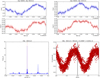 |
Fig. 1 Example of a periodic object. Top: light curves for the star 2113 for two consecutive nights in both R and I bands. Bottom left: ANOVA periodogram in the R band with the adopted period marked with the vertical dashed red line. Bottom right: phase curve. |
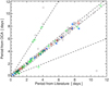 |
Fig. 2 Period comparison: the data from the literature, in particular S99 (blue asterisks), H02 (red crosses), and K23 (open circles), are compared with the periods determined in our current study. The dashed lines indicate the 1-to-l relationship as well as the values for the double and half periods. Approximately 90% of the sources are within the 20% threshold of agreement. Nevertheless, there are two notable deviations: in one case, the period determined is significantly longer (10.96 days) than the value found in K23, and in another it is significantly shorter (0.91 days); see text. |
5 Results
5.1 General statistics
Figure 3 shows the distribution of all 8197 stars and the fraction of 561 variables (7%) as a function of brightness. The variable sources and their properties are listed in Table F.1 (see Sect. 7). The completeness is determined to be about 16.5 mag in the I band and 17.5 mag in the R band.
It should be emphasized that the 561 variables correspond to 5σ detections. 147 out of 561 sources show periodicity with high probability. There are several ultrafast periodic objects, which are explained in more detail in Sect. 6. The amplitude of variability observed in our periodic variables can serve as a valuable, albeit crude, indicator of accretion activity. This correlation is consistent with features observed in TTSs within associations. The UBVRI photoelectric photometry catalog of TTSs by Herbst et al. (1994) reports that type I variables, which are stars with cool surface spots, have a maximum amplitude of 0.8 mag in the V-band and 0.5 mag in the I-band. However, Bhardwaj et al. (2019) has found that the average amplitude for PMS stars in the I band is approximately 0.5 mag, while the amplitudes for CTTS are estimated to be roughly twice the value compared to the WTTS in his sample.
Figure 4 shows the distribution of amplitudes for periodic and nonperiodic stars in both filters. The catalog of Herbst et al. (1994) shows that the majority of WTTS in I-band are periodic, with peak-to-peak variations of about 0.5 mag. On the other hand, CTTS generally show nonperiodic patterns and exhibit much greater variability. The importance of this strong variability is attributed to the significant influence of cool spots on the surfaces of K and M stars (e.g., H02; Venuti et al. 2015).
Since variability is one of the major properties of YSOs, in the following we concentrate on the 561 variable stars; their spatial distribution is shown in Fig. A.3.
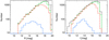 |
Fig. 3 Distribution of star brightness in R (left) and I (right) bands. The black lines represent the initial distribution of 13186 sources in R and 12898 in I. The green line illustrates the distribution of 11889 sources with matched light curves in both bands. The red line corresponds to 8197 stars identified by high-precision photometry with simultaneous detections in R, I, and 2MASS photometry with AAA qualifiers in JHK bands. The blue line represents the 561 variable sources. |
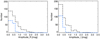 |
Fig. 4 Distribution of the amplitude of 549 variable stars measured by high-precision photometry, simultaneous detection in R (left) and I (right), and 2MASS photometry with AAA qualifiers in JHK. 402 non-periodic objects are shown in black. The blue distribution corresponds to the 147 periodic objects. |
5.2 Target selection (identification of young stellar objects)
To identify the YSOs in our sample, we cross-referenced the total list of 561 variable objects with primarily six catalogs. These include the Young Stellar Object VARiability (YSOVAR) catalog (Morales-Calderón et al. 2011, henceforth Mo-Call), the Spitzer Space Telescope Survey (Megeath et al. 2012), the studies of Fang et al. (2013) (Fnl3), and Fang et al. (2017) (Fnl7), the Vienna survey in Orion (VISION) catalog (Großschedl et al. 2019), as well as K23. Our findings include 162 objects from Mo-Call, 106 from Fnl3, 62 from Fnl7, and 208 from the recent study K23, with a few objects appearing in multiple studies (Cottaar et al. 2015; Briceno et al. 2018; Cottle et al. 2018; Hsu et al. 2012).
The color-color diagram (CCD), the color-magnitude diagram (CMD), and the kinematics information provide a global picture of the photometric properties of the candidates and are useful when identifying stars associated with a cluster. An optical CMD and an NIR CCD were used to classify our variable candidates (Bhardwaj et al. 2019; Lata et al. 2016).
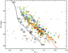 |
Fig. 5 Color-color diagram (H – K, J – H) for 561 variable stars. The NIR colors are from the 2MASS Point Source Catalog. Green dots: 162 objects matched to Mo-Call, Blue dots: 106 objects matched to Fnl3, Red dots: 62 objects matched to Fnl7, Yellow dots: 267 objects matched to K23, Megeath et al. (2012), Großschedl et al. (2019), and others (see text). Black dots: 105 objects without any youth indicator in the literature. Bona fide TTS are marked by crosses; CTTS (red), WTTS (blue). The solid curve represents the locus of main-sequence stars from Kenyon & Hartmann (1995); the red dashed lines are reddening vectors for AV = 10 mag. The black dash-dotted line is the locus of unreddened CTTS from Meyer et al. (1997). |
5.3 Color-color diagram
Figure 5 shows the NIR CCD for 561 variables with colors from the 2MASS point source catalog. The solid curve represents the intrinsic colors for main sequence stars (Ducati et al. 2001). The dashed lines are reddening vectors for AV = 10 mag. While most stars have colors of normally reddened stars, less than 5% lie to the right of the lower reddening line for main sequence stars and below the locus of unreddened CTTS (dash-dotted line), indicating IRE.
A considerable number of CTTS are found within the reddening band, some of which even overlap with WTTS. However, the presence of CTTS in this area does not necessarily mean that there is no IRE. To accurately determine the presence of IRE, additional information is needed about the extinction of the stars or their underlying spectral types. Those stars lying above the upper reddening line are most probably giant stars. The presence of stars below the de-reddened CTTS locus and to the right of the main-sequence branch in Fig. 5 can be attributed to the circum-stellar disk models proposed by Lada & Adams (1992). In this region of CCD, the modeled systems with stellar surface temperatures between 3000 and 12000 K can occupy such positions. In addition, two CTTS are observed in this region. One CTTS is completely below the locus of unreddened CTTS, while the other CTTS is closely aligned with the locus but has a significant excess in H-K color.
The 105 variable stars without a youth indicator populate the same areas as the previously known bona fide YSOs, suggesting that they could also be YSO candidates.
5.4 Color-magnitude diagram
CMDs are a valuable tool to study the evolutionary stage of stars. In Fig. 6 we show the comparison between R and R – I CMD, which shows the distribution of about 561 variable objects in our FoV with available photometric data in both R and I bands, with sources with known spectral types standing out. The variable objects are marked as large symbols; the isochrone refers to an age of 3 Myr (Baraffe et al. 2015). More than 90% of our sources are located in a specific region that shows a strong correspondence with the location of YSOs in the enclosed area, as shown in Fig. 46 of Fn13. By using the locations of established YSOs, we can effectively identify potential YSO candidates. However, this generosity of selection may inadvertently include reddened field stars, thus contaminating the sample of YSO candidates.
The median R – I color for all variables is approximately 1.09. However, in the case of our variables examined in Fnl3 (primarily in the L1641 region), the median R – I color is around 1.16, which is slightly redder or cooler. For objects identified in Fnl7 (mainly in the NGC1980 region), the median R – I color is even redder, at 1.34. The median R – I value for objects identified in the K23 study is about 1.10, which is closer to the value for all variables. The data from the K23 study covers a broader region, which includes the areas studies in Fnl3 and Fnl7. Approximately 45% of the Fnl3 sample and about 63% of the Fnl7 sample overlap with our objects that were also identified in conjunction with K23. It’s worth mentioning that about two-thirds of the K23 objects do not overlap with objects common to either Fnl3 or Fnl7. Note that in our sample of variables, the fraction of CTTS for the Fnl3 region is approximately 44%, while for the Fnl7 region, it is 25%. For the objects identified in the K23 study that overlap with our list, this fraction is slightly more than 50%. Additionally, our observations cover a broad region that extends southward to NGC1977.
Kounkel et al. (2017) found a CTTS fraction  of 0.29 by studying Hα observed sources within the NGC 1980 region, among other studies in this area. However, Bouy et al. (2014) had different CTTS fractions for NGC 1980, as they covered a slightly broader region. They also questioned the relationship of NGC 1980 to ONC, especially with respect to L1641. Pillitteri et al. (2013) also supported this claim by showing a different X-ray luminosity between NGC 1980 and L1641. Low-mass star formation theory traditionally suggests that CTTS evolve into WTTS as their circumstellar disks disintegrate over a period of several million years; consequently, WTTS should be older than CTTS. However, practical studies of young clusters show that the TTS members within a cluster have a wide age range, so the differences are blurred. The age range is partly due to errors in both observable quantities and theoretical isochrones. In Taurus, Hartmann (2001) found no statistically significant difference between the age distributions of CTTS and WTTS. The same result was reported by Herbig (1998) for IC 348 and by Herbig & Dahm (2002) for IC 5146. Similarly, Dahm & Simon (2005) found a similar mean age for CTTS and WTTS in NGC 2264. The mean age of the CTTS group is even slightly higher than that of the WTTS group. Thus, the Hα emission is obviously not a reliable age indicator. In fact, the transition from CTTS to WTTS depends on the timescale of disk evolution, and this timescale varies from star to star. Accordingly, one should expect to find both CTTS and WTTS with similar ages in a population of the same age, as the timescale of disk evolution varies.
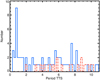 |
Fig. 6 R vs. R -ICMD for objects in the FoV. Green dots: 162 objects from Mo-Call. Blue dots: 106 objects matched to Fnl3. Red dots: 62 objects matched to Fnl7. Yellow dots: 267 objects matched to K23, Megeath et al. (2012), Großschedl et al. (2019), and others (see text). Black dots: 105 stars without any youth indicator in the literature. Bona fide TTS are marked by crosses; CTTS (red), WTTS (blue). The red curve is an isochrone of 3 Myr (Baraffe et al. 2015) for a distance of 412pc. The black line correspond to the main sequence from Ducati et al. (2001). Ultrafast rotators (P < 0.5 days) are marked with open squares (see Sect. 6.2). |
 |
Fig. 7 Period distribution for 20 bona fide CTTS (red) and 67 WTTS (blue); classification from Fnl3, Fnl7 and K23. |
5.5 Period distribution of bona fide TTauri stars
Cool extended regions, similar to sunspots, are mainly considered to be the source of variability in both T Tauri classes, while hot spots are only found in CTTS. This is due to the thick circumstellar disk (e.g., Fernandez & Eiroa 1996; Biddle et al. 2021) from which gas falls along magnetic field lines onto the stellar surface. Hot spots form at the impact points, which are usually small. Both the cool and hot spots cause stellar rotation to produce periodic variations in the star’s light curve over a period of hours to days; the superposition of the two effects can produce complicated patterns of variability. During periods of more violent accretion, larger hot spots are created, increasing the contribution to the light curve variations and leading to inflated amplitudes. Similarly, the higher temperatures of the hot spots lead to additional color variability due to increased emission at shorter wavelengths.
Figure 7 shows the period distribution for 20 bona fide CTTS and 67 WTTS of the present study; the corresponding classification was mostly adopted from Fnl3 and Fnl7, and K23. The results are consistent with the findings of Edwards et al. (1993), who found that WTTS have rotation periods of 1.5 < Prot < 16 days, with a significant number of objects having Prot < 4 days. In comparison, the majority of CTTS has rotation periods Prot > 4 days (see also Serna et al. 2021).
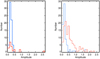 |
Fig. 8 Amplitude distribution for bona fide TTS. Left: 87 periodic objects, 20 CTTSs (red), and 67 WTTSs (blue). Right: 195 nonperi-odic objects, 122 CTTSs (red), and 73 WTTSs (blue). The classification is taken from Fnl3, Fnl7, and K23. |
5.6 Amplitude distribution of bona fide TTauri stars
The distribution of amplitudes of periodic TTS and nonperiodic TTS are shown in Fig. 8. The statistics of the periodic objects are rather poor, mainly because only 20 CTTS are available. If we try to estimate something like a trend, we can say that all WTTS have small amplitudes below 0.5 mag (actually below 0.3 mag), while the CTTS reach larger amplitudes, in one object more than 2.5 mag. This could indicate a difference between the two classes, in the sense that the rotation of the cool spots dominates the brightness variations of the WTTS, while the rotation of the hot spots is occasionally seen in the CTTS. On the other hand, the amplitudes of the nonperiodic objects in both CTTS and WTTS show a clear peak at small amplitudes below 0.5 mag. While over 38 percent of CTTS show amplitudes greater than 0.5 mag, few WTTS show such large amplitudes, indicating significant physical differences in the causes of variability between CTTS and WTTS. This can be interpreted as a consequence of occasional accretion in both classes masking the underlying brightness modulation by rotation.
5.7 Spectral index, α
Due to the small number of classified TTSs in the present sample, we used the spectral index, α, between 2.2 (2MASS) and 12 µm (W3) from the Wide-field Infrared Survey Explorer (WISE) as the class discriminator. In this scheme, the spectral energy distributions (SED) is expressed as log(λFλ) vs. log(λ) and follow the definition of the index, α, implemented by Lada &Wilking (1984) as
 (9)
(9)
Almost a decade later, Greene et al. (1994) revised this scheme because more detailed observations refined the definitions of SED classes to better adapt to physical stages of YSO evolution. They found that YSOs with α ≥ −0.3 have NIR spectra which are strongly veiled by emission from hot dust and thus a typical of TTS stars. It is therefore likely that YSOs with −0.3 > α > −1.5 are PMS stars with considerable circumstel-lar dust that does not veil their photospheres in the NIR. Greene et al. (1994) also showed that the spectral indices α obtained from data at 2.2 and 20 µm show no systematic deviations from those derived from 2.2 and 10 µm. This suggests that the W3 filter from WISE will be suited too. Therefore, the following indices are used throughout the present work:
Class I sources have α > 0.3 and have SEDs broader than a blackbody which are rising longward of 2 µm, while Class Flat objects have −0.3 ≤ α ≤ 0.3. Class II sources have −1.6 ≤ α ≤ −0.3 and have SEDs broader than a blackbody but which are flat or decreasing longward of 2 µm. Eventually, Class III sources have α < −1.6 and have SEDs that can be modeled with reddened blackbodies with no or small NIR excess emission.
The current sample is divided into two groups. The first group consists of 456 sources confirmed as YSOs in previous literature, with the highest overlap observed in the data from K23, Megeath et al. (2012), and Großschedl et al. (2019). Additionally, there is some overlap among the four studies; within our known YSOs list, 70 objects are common in K23 and Mo-Call, 58 objects in K23 and Fnl3, and 23 objects in K23 and Fnl7. Furthermore, 17 objects are common in the studies of Fnl7 and Fnl3, while 16 objects are shared between Fnl7 and Mo-Call. In addition, there are 59 objects identified in Großschedl et al. (2019) that are not listed in the previous studies.
Object 3241 of our list, is classified as WTT in Fang et al. (2009) while it is classified as CTT in Fnl7; we consider this object as WTT due to its spectral index value. The second group comprises 105 objects, with α values obtained in this work, classifying them as YSO candidates.
The use of W3 photometry presents challenges; however, the photometry results are generally reliable. We verified the W3 photometry for the 561 variable sources and found that only 12 objects, including 3 periodic ones, lacked reliable values due to excessively large errors, unrealistically small errors, or missing values entirely. We also reviewed the W3 images of the periodic sources and confirmed the quality reported in the catalog. Considering the object classes, the count of variable sources decreases to 549, as missing W3 values preclude classification, and the number of periodic objects is reduced from 147 to 144.
Figure 9 shows the distribution of a for all 549 variable objects. In general, both periodic and nonperiodic objects are mainly distributed over Class II and III. However, the distribution of periodic objects has a clear maximum at α ∼ −2 to −2.5; this yields 96 objects (66.7%) in Class III and 44 objects (30.6%) in Class II. Additionally there are four objects (less than 3%) in Class Flat. In contrast, the nonperiodic objects show a bimodal distribution with a strong maximum at α ~ −1 and a smaller maximum at α ~ −2.2. This translates into 143 objects (35%) in Class III, 224 objects (55%) in Class II, 28 objects (7%) in Class Flat, and 10 objects (more than 2%) in Class I.
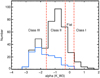 |
Fig. 9 Distribution of α for 549 variables. The spectral index, α, has been determined between 2.2 µm (2MASS) and 12 µm (W3, WISE). The black and blue histograms shows the 405 nonperiodic and 144 periodic objects, respectively. The boundaries between the classes are marked as red dash-dotted lines. |
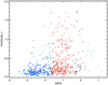 |
Fig. 10 Variability amplitude as a function of the spectral index, α. Blue points represent Class III objects, red points indicate Class II objects, green points are Class I objects, and black points Class Flat objects. Class II objects generally show higher variability amplitudes compared to other classes, especially notable in nonperiodic objects (see the text). |
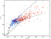 |
Fig. 11 J − H, H − K color–color diagram for 561 variable stars. Class Flat and Class I sources (black dots), Class II sources (red dots), Class III sources (blue dots). The classified TTS are marked as crosses; CTTS (red), WTTS (blue). The dash-dotted line marks the locus of unreddened TTS (Meyer et al. 1997). The solid curve represents the locus of main- sequence stars from Kenyon & Hartmann (1995). |
5.8 Amplitude distribution of selected T Tauri stars based on the spectral index, α
Figure 10 shows the variability amplitude as a function of the spectral index, α. Notably, a larger amplitude of variability is observed in Class II objects. This trend indicates that Class II sources show more dynamic and variable behaviors than their counterparts. In the context of periodic variability, there are minimal differences between Class II and Class III sources. However, the situation contrasts sharply when considering nonperiodic objects. In these cases, Class II sources shows higher variability, with mean and median values at 0.6 and 0.4, respectively. In contrast, Class III sources show markedly lower variability, with mean and median values of 0.25 and 0.14, respectively. This is consistent with the results shown in Fig. 8, concerning bona fide TTS, suggesting that periodic physical processes influencing variability might be similar across these classes. The pronounced difference between the clasess suggest the potential influence of underlying mechanisms, such as disk presence or accretion activities, which are more prevalent in Class II objects and could account for their enhanced variability.
5.9 Near-infrared colors and the spectral index, a
Figure 11 shows the same J − H, H − K color–color diagram as Fig. 5. This time the sources are marked according to their spectral index, a. At first glance there is a significant separation between Class II and Class III sources at around H − K ≃ 0.2 with Class II sources in the redder part and Class III sources in the blue part of the diagram (see also Dahm & Simon 2005).
Among the 310 objects classified as classes I, flat, and II, approximately 18% are found to lie to the right of the main- sequence reddening line, linked to IRE, which may feature emission from circumstellar disks. This estimate likely underestimates the population of disked objects since many CTTSs that fall within the range of normal reddened stars exhibit distinct from mean of WTTs NIR colors J − H ~ 0.7 and H − K ~ 0.25, indicating the presence of a diskless or poorly developed disk population. While the position in the JHK diagram depends sensitively on the inner disk properties, i.e. J − H measures the amount hot dust, a measures the amount of cooler dust. A a vs. H − K diagram, which is divided into the IR classes, can be found in Fig. A.4.
5.10 Periods of Class II and Class III sources
Figure 12 shows the period as a function of α for 144 objects. The 18 out of 20 CTTS have −1.55 < α and thus cover the range of Class Flat and Class II sources while 50 out of 67 WTTS are Class III sources with α <−1.55. One object has been identified as a CTTS in Fn13, despite the spectral value being –1.88. On the other hand, while two periodic objects with the highest a are recognized as WTTS in K23, there is one identified as a CTTS in K23, with α of −2.81 translating to Class III sources.
There are two clear cutoffs in the period distribution, despite the good sensitivity to periodic signals for periods both longer and shorter than the observed cutoffs. At the long period end, the distribution tapers off strongly for P > 8 days. This agrees with the results by S99 and K23, closely resembling the observed long-period cutoff in the distributions of other young clusters. At the short-period end, the distribution drops dramatically for P < 0.5 days with 9 sources (~6%) below that limit. For the star in the present sample, with M* ≃ 0.6 M⊙ and R* ≃ 2.2R⊙ according to the PMS tracks of Siess et al. (2000), the rotation period corresponding to breakup velocity is ~eq0.5 days. Therefore, the short-period cutoff can be ascribed to a real physical limit on the minimum rotation period for the stars in the present sample. Most periods (35%) are clustered in the range 0.5 ≤ P ≤ 2 while 34% are evenly distributed between 4 and 8 days.
Figure 13 shows the period as a function of H − K for 147 objects. Most sources populate the region 0.10 < H − K < 0.25, among them 56 bona fide WTTS and 21 Class II sources. Three Class III and one Class II are slightly bluer with H − K < 0.1. The region H − K > 0.25 is dominated by 26 Class II sources, among them 13 bona fide CTTS and 6 Class III sources. This color behavior was already apparent from Fig. 11 where Class II sources and CTTS tend to be redder than Class III objects and WTTS.
There are 44 sources have P < 1.5 days (31%). The period distribution of 82 sources between 1.5 and 8 days is fairly uniform. As in Fig. 12 there are 18 sources with P > 8 days. At the short-period end, there are 9 objects with P < 0.5 days.
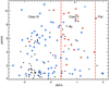 |
Fig. 12 Period as a function of α for 144 objects. The classified TTS are marked as crosses with CTTS and WTTS shown as red and blue, respectively. |
5.11 Amplitudes for Class II and Class III sources
Figure 14 shows the amplitude as a function of H − K for 144 periodic and 405 nonperiodic objects. There are 44 periodic and 224 nonperiodic Class II sources, 96 periodic and 143 nonperiodic Class III sources, and 4 periodic and 28 nonperiodic Class Flat and 10 class I sources without period signature. Despite a wide overlap between the different classes there is a concentration of Class III sources in the blue (0.1 < H − K < 0.25) region with amplitudes below I ~ 0.4 mag while Class II sources populate the region H − K > 0.1 mag with an amplitude scatter increasing with H − K up to ΔI ~ 2.5. The highest amplitude for known WTTS in the sample belong to the class II of our classification; Object 4437, identified as Class Flat in Fn13. The subsequent WTTS, with an amplitude exceeding 1 mag is object 6911 in our list and classified in the Kounkel et al. (2017).
Most sources populate the region 0.1 < H − K < 0.25, among them 105 of all 140 WTTS are located in this part of plot, in contrast to CTTS of which only 23 out of 142 are in this range of H − K color; mostly they are located in 0.30 < H − K < 0.55.
There are 153 sources among 224 Class II nonperiodic objects are in the range 0.15 < H − K < 0.55 whereas periodic objects are more concentrated; 38 out of 44 periodic stars are located in 0.15 < H − K < 0.45. Both periodic and nonperiodic Class III objects have mostly 0.1 < H − K < 0.25; 87 of all 96 periodic objects and 95 of all 143 nonperiodic stars have this range of color. Finally, there is no considerable difference in the distribution of those objects which have youth indicator and those which have not.
Figure 15 plots the amplitude of the variables in R against the difference of it in R and I including color coding by class. The solid line is the line along which the points would fall if the amplitudes in both bands were identical. About 10% of objects vary with amplitudes more than 1 mag, but a more typical amplitude for the variables is 0.2–0.5 mag. There is a slight indication that Class flat objects may have slightly larger average amplitudes. However, when considering the mean amplitudes in the R band for Class I, flat, and II among nonperiodic objects, the values are 0.51, 0.54, and 0.51 mag respectively, showing no significant difference. For Class II and flat among the periodic group, the mean amplitudes are 0.30 and 0.31. This suggests that any tendency toward larger amplitudes in more embedded SEDs is likely subtle or obscured by limited sample sizes. Notably, Class III objects exhibit significant differences in both samples. The mean amplitude for Class III variables is 0.18 in the nonperiodic sample and 0.20 in the periodic list, indicating a distinct deviation from the rest of the distribution. It is worth mentioning that the lower value observed for class III nonperiodic objects is attributed to the difficulty in detecting periodicity in objects with lower amplitudes.
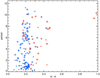 |
Fig. 13 Period as a function of H − K. Class II (red dots), Class III (blue dots). The classified TTS are marked as crosses with CTTS and WTTS shown as red and blue, respectively. |
5.12 Period distribution
The distribution of periods was heavily debated between S99 and H02 for over two decades. More recently, K23 unveiled the period distribution for a significantly larger sample in this region based on TESS light curves. Figure 16 illustrates the period distribution for ONC as derived from the studies of K23, S99 and H02 alongside the new results from this work. As highlighted in Sect. 4, a substantial overlap exists between our study and K23. However, about 57% of our periodic objects are not encompassed by K23.
In order to gather up-to-date information, we retrieved the TESS light curves for our periodic objects which led to the identification of a further 28 objects on our list. Very generally, the small period values prevail in all studies. The distributions of S99, H02 and K23 show a clear maximum at around 2 days. We find that the peak of the distribution is dominated by stars with periods below 1 day. The relative abundance of stars with periods ≤ 2 days is comparable in all three studies − 35% (this work), 27% (K23) 24% (H02) and 24% (S99). If only periods ≤1 day are considered the percentages are 20% (this work), 11.5% (K23) 5% (H02) and 9% (S99). In other words, the occurrence of very short periods in the present work is almost a factor of two to four higher than in the studies by S99, H02 and K23. This result is a consequence of the exceptional dense time sampling employed in this study and the presence of fast rotating objects not included in K23. The fastest object reported in S99, object 11224 in our list, with period 0.27 days which is confirmed in this work by the value 0.28 days, but it is absent in K23; This object is the faintest object (I = 15.71496 mag) and has the highest amplitude (ΔI = 0.73597 mag) among the objects with P < 1 day in our list; this object also identified by Pillitteri et al. (2013) as a young X-ray star.
The variability of the stars was distributed over three amplitude groups: 242 stars with ΔI < 0.2 mag, 179 stars with 0.2 < ΔI < 0.5 mag, 135 stars with 0.5 < ΔI < 1.75 mag, and 5 objects with ΔI > 1.75, while these numbers for periodic objects are 85, 55, 6, and 1, respectively. We found that 14 out of 67 bona fide WTTS have period values between 0.5 and 1 days. On the other hand, we have identified there is no bona fide CTTS with period shorter than 2 days; Furthermore We discovered that there are only seven objects with a period greater than 10 days. Marilli et al. (2007) studied 39 WTTS in the Orion star-forming region, and determined that, although there may still be slowly rotating single stars within the sparse population of Orion WTTS, they appear to be notably less compared to the ONC. Additionally, they did not identify a clear correlation between rotation period and age among the investigated objects.
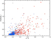 |
Fig. 14 Amplitude as a function of H − K. Periodic objects (dots), nonperiodic objects (diamonds). Class Flat and Class I sources (black symbols), Class II (red symbols), Class III (blue symbols). The classified TTS are marked as crosses with 142 CTTS and 140 WTTS shown as red and blue, respectively. |
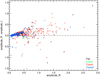 |
Fig. 15 Amplitude variations across the SED classes, color-coded for each class. The amplitude distributions across these classes are statistically indistinguishable. |
6 Discussion
6.1 Implications of variability and periodicity
We find that of 405 nonperiodic variable objects, 32 have an amplitude greater than 1 mag in both the I and R bands. Of the 147 periodic variable objects, there is one with an amplitude greater than 1 mag in both the I and R bands. This clearly shows that nonperiodic objects tend to have high amplitudes. This pattern is usually attributed to the accretion process, which normally makes it impossible to calculate the rotation period of an object (Rodríguez-Ledesma et al. 2009; Park et al. 2021; Wang et al. 2023). Additionally, sudden changes in brightness can lead to aperiodic behavior, potentially caused by changes in extinction (Fischer et al. 2023).
Figure 17 illustrates the relationship between period and R − I color. Class II sources predominantly exhibit periods greater than 2 days, in contrast to Class III sources, which show a more uniform distribution across various periods. When analyzing only Class II sources with periods exceeding 2 days, a clear positive correlation between period and R − I color becomes evident. These findings lend support to the hypothesis that Class II objects, which possess circumstellar disks, generally rotate more slowly compared to Class III objects that typically lack such disks. The slower rotation of Class II objects can be attributed to their being dynamically locked with their disks, resulting in angular momentum loss, or to having lost significant angular momentum during the disk-locking phase. These stars are typically more massive than those exhibiting faster rotation, as observed in NGC 2264 (Lamm et al. 2005).
For the objects that match between our sample and the Fn17 sample, the median period is 1.92 days, and the median amplitude in the I band is 0.17 mag. Conversely, for the objects common to the Fn13 sample, these values are 4.24 days and 0.25 mag, respectively. As discussed in Sect. 5.4, the subgroup of our periodic objects that overlap with Fn17 consists predominantly of WTTS. These stars are more evolved, have typically been released from their circumstellar disks, and thus exhibit shorter periods and lower amplitudes. In contrast, the sample from Fn13, which contains a higher proportion of CTTS, shows longer periods and larger amplitudes due to these stars being dynamically locked to their disks. This observation supports the star formation scenario where CTTS, characterized by higher accretion rates and more substantial circumstellar disks, eventually deplete their disks and evolve into WTTS, which exhibit lower accretion rates.
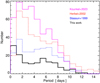 |
Fig. 16 Distribution of periods in ONC. This work (black), S99 (blue), H02 (red), and K23 (magenta). |
6.2 Identification of fast rotators as young stellar objects
As can be seen in Fig. 16, the distribution of periods determined in earlier studies (S99, H02 and K23) shows a clear peak at around 2 days. The sources with periods of less than 2 days are considered fast rotators. In our study, of the 52 objects with periods of less than 2 days, 21 objects are bona fide WTTS and one is a bona fide CTTS. From the 30 objects with periods of less than 1 day, 14 are bona fide WTTS, thus representing a larger proportion of more evolved objects. The distribution peaks at about 1 day, with about 40% being less than half a day.
The interpretation of ultrafast rotating hot/cold spots (P < 0.5 days) is a challenge. There are 12 objects whose period is very close to or less than 0.5 days. Six of them are close to the MS (see Fig. 6). At the age of <1 Myr, fast rotators tend to have rotation periods between 1 and 2 days (K23). Similar behavior has been observed in the ρ Ophiuchus cluster (~1 Myr), where the period distribution peaks at approximately 1.5 days (Rebull et al. 2018). However, with increasing age, the proportion of systems with periods <1 day increases relative to the total number of stars. This process seems to continue at older ages, as in populations older than 20–30 Myr, most fast rotators seem to favor periods <0.5 days (Kounkel et al. 2022). However, the other six objects do not follow this hypothesis, as they are far away from the MS and are located between all the other young periodic objects (see Fig. 6). The WTTS are also still in a contractive evolutionary phase. If they are in the process of magnetic decoupling from their (rotation-breaking) disk, a sudden “overshooting” of the contraction could occur, leading to the observed extremely short rotation periods, which may relax in the course of further evolution. The ultrafast rotation raises new discussions for the theoretical models of angular momentum evolution and some physical concepts such as the stability of the star (e.g. Goupil et al. 2006).
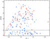 |
Fig. 17 Distribution of periods vs. R − I color. Class flat sources are indicated in black, Class II sources in red, and Class III sources in blue. The CTTS and WTTS are marked with red and blue crosses, respectively. The red dashed-dotted line represents the median of the period within a 0.1 bin size in the color R − I, taking into account periods over 2 days (horizontal black dotted line). |
6.3 Fast rotators and challenges
Our periodic sample includes three objects identified as eclipsing binaries in Drake et al. (2014), with data from the Catalina Realtime Transient Survey (CRTS). The light curves and analyzes for these objects (632, 10304 and 10845) are described in detail in Appendix C (available on Zenodo). We estimate the periods for objects 632 (Fig. C.1), 10304 (Fig. C.3) and 10845 (Fig. C.4) to be 0.197, 0.139 and 0.188 days, respectively. Their phase light curves reveal a non-eclipsing binary nature, and the short periods are clearly visible in the intranight light curves, exemplified by source 632 in Fig. C.2. The intranight light curves of the other objects are similar and are therefore not shown. Assuming radii of 1 R⊙ and masses of 1 M⊙ for these stars and a period of about 0.2 days, we estimate a breakup velocity of about 437 km/s. Assuming a maximum inclination of 90 degrees for the stars’ rotational axes relative to our line of sight, the observed rotational velocities are about 267 km/s. Thus, the rotational velocity is therefore about 61% of their breakup velocity. This indicates that the stars are rotating at a significant fraction of the speed at which they would begin to lose mass due to centrifugal forces, suggesting that they are rotating quite rapidly relative to their maximum stable rotational velocities. This percentage is considerably high. However, there is evidence of stellar rotation in YSOs at about 90% of breakup velocity, such as HD 135344B (Müller et al. 2011).
Fast rotating MS stars are typically those condensed from gas clouds without losing much angular momentum. In contrast, there are also slowly rotating stars on the MS that have a wide range of rotation periods. This suggests that these slower stars have lost a significant amount of angular momentum during their earlier TTS phase. The rotational evolution of PMS stars is commonly examined through two distinct scenarios: First, there is the concept of disk-locking, where stars maintain a constant rotation period due to their interaction with circumstellar disks, resulting in a pronounced rate of angular momentum dissipation (Lamm et al. 2005). The main question revolves around the temporal evolution of the period distribution and the time of separation of the stars from their disks. As can be seen from H02, the estimated half-life of the star-disk interaction is 0.7 Myr. Our observations cover a heterogeneous range of ages within the Orion association, with a median age distribution of 3 Myr (see isochrone in Fig. 6). Consequently, our sample includes a significant proportion of objects that have undergone a longer star-disk interaction, and our particular temporal sampling strategy allows us to identify more evolved objects that are dissipating from their circumstellar disk and have shorter periods. For example, the fast rotators seen near the MS in Fig. 6) and discussed in Sect. 6.2). Second, there is the phenomenon of spin-up, in which stars undergo accelerated rotation without significant loss of angular momentum. Between these two scenarios, there are some stars that lose angular momentum without being tightly bound to their disks at a fixed rotation period, with a lower loss rate (moderate) compared to strict disk-locking cases.
Hartmann (2002) suggested that disk- locking does not occur instantaneously, but develops over time. This duration is influenced by the rate at which angular momentum is extracted from the inner disk. The stars undergoing magnetic interaction with their disks but with ages shorter than the disk-locking achievement time scale do not maintain a constant rotation period (they are spinning up). However, as long as the magnetic star-disk interaction persists, it continues to extract angular momentum from the stars, albeit at insufficient rates to achieve disk locking. Consequently, these stars experience a deceleration in their spin-up rate (due to contraction) and rotate with periods shorter than the disk-locking period but longer than those of stars conserving angular momentum during spin-up. This scenario of moderate angular momentum loss, driven by magnetic forces, can persist as long as the magnetic star-disk interaction endures, corresponding to a stellar age smaller than the dissipation time of the circumstellar disks. It’s plausible that stars in ONC, which consists of a considerable fraction of young objects with approximate age <10 Myr (as reported in K23), have not yet achieved disk-locking. Therefore, the existence of rapidly rotating stars in the ONC could be attributed to disk-locking achievement times exceeding their ages. There is one short-period object in our list (object 8187) that shows the higher excess in R − I and could be explained by this scenario. Fast rotating stars with large IREs have also been observed in S99 and H02.
Studies on other young stellar clusters and associations indicates a common trend where, on average, stars with disks tend to rotate more slowly, though a small number of them rotate faster than about 2 days (Rebull et al. 2018, 2020). Additionally, the variability amplitude tends to decrease with stellar age, and typically, higher-mass stars exhibit lower amplitudes compared to their lower-mass counterparts. Specifically, Rebull et al. (2018) observed that circumstellar disks are mainly associated with slower-rotating M stars, and only rarely with disks exhibiting rotation periods around 0.5 days (see their Fig. 8). However, M dwarfs with disks generally rotate faster than FGK stars with disks. For four such M dwarfs, Rebull et al. 2018 provided direct evidence supporting the disk-locking mechanism.
7 Conclusions
We have presented the results of an extensive photometric survey with high temporal resolution carried out on a six-square-degree region centered on NGC 1980 in the Orion Nebula. We used a unique observational setup that allows us to obtain high-quality light curves with time sampling on the order of minutes. This is the first time that such an intensive ground-based photometric campaign has been carried out in the Orion Nebula. Our results can be summarized as follows:
We have successfully determined rotation periods for a substantial sample of 147 sources, revealing a wide range from 0.2 days to several days. Surprisingly, a significant majority of these objects, 134 out of 147, display amplitudes below 0.5 mag. This consistency aligns with the amplitude of variation typically attributed to surface spots on young stars;
We have found a notable disparity in the number of fast rotators in comparison to previous studies. For a high percentage of fast rotators, the peak of their rotation distribution occurs at periods below 1 day. Our findings show that these ultrashort periods occur at a rate two to four times higher than previously estimated. This disparity, particularly in comparison to studies by Stassun et al. (1999), Herbst et al. (2002), and Kounkel et al. (2023), highlights the uniqueness of our dataset obtained with an exceptional time sampling strategy, a method meticulously designed to capture variability on scales ranging from mere hours to expansive periods spanning years. Moreover, the fact that our field of view is considerably large and the fact that Orion is a heterogeneous association with many different aged populations means that it is possible to detect YSOs in different stages of evolution;
We have identified a distinct subgroup among the ultrafast rotators, signifying a crucial evolutionary phase. These objects, situated in the final stages of their evolution along the main sequence, exhibit considerable spin-up, likely due to the dissipation of their disks. Additionally, our analysis of the CMD has unearthed a group of ultrashort period objects;
We have identified a significant population (10%), primarily originating from WTTSs, characterized by rotation periods of less than 1 day, which is absent in prior studies;
We have observed that the young periodic objects, despite their youthful age, display significant expansion and higher luminosity concerning their spectral types. This discovery challenges conventional expectations and invites further inquiry into the mechanisms governing their evolution.
Data availability
Appendices B-E are available on Zenodo with the https://zenodo.org/records/13899195. Table F.1 is available at the CDS via anonymous ftp to cdsarc.cds.unistra.fr (130.79.128.5) or via https://cdsarc.cds.unistra.fr/viz-bin/cat/J/A+A/691/A358.
Acknowledgements
We thank Marina Kounkel for providing the detailed table with the coordinates, periods and classification of the YSOs analyzed in Kounkel et al. (2023). We thank the anonymous referee for their insightful comments and suggestions, which have helped improve the manuscript. We would like to express our deep gratitude to Dr. Francisco Pozo Núñez for his invaluable advice and guidance throughout this project. This work was supported by the Nordrhein-Westfälische Akademie der Wissenschaften und der Künste, funded by the Federal State Nordrhein-Westfalen and the Federal Republic of Germany. ZC is supported by the National Natural Science Foundation of China with grant No.12373030. This research has made use of the SIMBAD database, operated at CDS, Strasbourg, France. This paper includes data collected by the TESS mission. Funding for the TESS mission is provided by the NASA’s Science Mission Directorate.
Appendix A Overview of observational data
Figure A.1 shows the field of view of 2.4° × 2.4° with Iota Ori- onis in the center. In the region around RA = 83.8 deg and Dec = –5.4 deg, our optical imaging suffers from large extinction, resulting in the detection of only a few stars. The identification of variable objects using three different methods is shown in Fig. A.2. As shown in Fig. A.3, the periodic and nonperiodic objects exhibit a similar spatial distribution. Figure A.4 shows the spectral index, α, as a function of H – K.
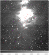 |
Fig. A.1 Field of view of 2.4o × 2.4° with Iota Orionis in the center of the field. All periodic objects identified in this work are marked with red dots and the fast rotators are superimposed with blue circles. |
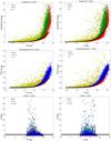 |
Fig. A.2 Identification of variable objects with three different methods for the filters R and I. The diagrams on top and in the middle show the amplitude and S D methods respectively. For both methods, the threshold varies exponentially because the scatter and noise are higher for weak objects. The lower diagrams show the J–index method. We established an empirical threshold of 1.35 after conducting a detailed examination of the light curves for variable candidates that were also detected using other methods. This threshold was further refined by eliminating spurious detections. |
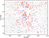 |
Fig. A.3 Spatial distribution of YSOs in the field of view. The red dots represent 561 variable objects with 5σ detections, the blue dots show 147 periodic objects. |
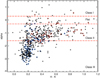 |
Fig. A.4 Spectral index, α, as a function of H – K. The periodic objects and the nonperiodic objects are shown with dots and squares respectively. The classified TTS are marked as crosses, CTTS and WTTS are shown in red and blue respectively. |
References
- Attridge, J. M., & Herbst, W. 1992, ApJ, 398, L61 [NASA ADS] [CrossRef] [Google Scholar]
- Bhardwaj, A., Panwar, N., Herczeg, G. J., et al. 2019, A&A, 627, A135 [NASA ADS] [CrossRef] [EDP Sciences] [Google Scholar]
- Baraffe, I., Homeier, D., Allard, F., et al. 2015, A&A, 577, A42 [NASA ADS] [CrossRef] [EDP Sciences] [Google Scholar]
- Barnes, S., & Sofia, S. 1996, ApJ, 462, 746 [Google Scholar]
- Bertin, E. 2006, Astronomical Data Analysis Software and Systems XV, 351, 112 [NASA ADS] [Google Scholar]
- Bertin, E., & Arnouts, S. 1996, A&AS, 117, 393 [NASA ADS] [CrossRef] [EDP Sciences] [Google Scholar]
- Bertin, E., Mellier, Y., Radovich, M., et al. 2002, Astronomical Data Analysis Software and Systems XI, 281, 228 [Google Scholar]
- Biazzo, K., Melo, C. H. F., Pasquini, L., et al. 2009, A&A, 508, 1301 [NASA ADS] [CrossRef] [EDP Sciences] [Google Scholar]
- Biddle, L. I., Llama, J., Cameron, A., et al. 2021, ApJ, 906, 113 [NASA ADS] [CrossRef] [Google Scholar]
- Bouma, L. G., Jayaraman, R., Rappaport, S., et al. 2024, AJ, 167, 38 [NASA ADS] [CrossRef] [Google Scholar]
- Bouvier, J. 1990, AJ, 99, 946 [NASA ADS] [CrossRef] [Google Scholar]
- Bouvier, J., Cabrit, S., Fernandez, M., et al. 1993, A&A, 272, 176 [NASA ADS] [Google Scholar]
- Bouy, H., Alves, J., Bertin, E., et al. 2014, A&A, 564, A29 [NASA ADS] [CrossRef] [EDP Sciences] [Google Scholar]
- Briceno, C., Calvet, N., Hernandez, J., et al. 2018, arXiv e-prints [arXiv:1805.01008] [Google Scholar]
- Carpenter, J. M., Hillenbrand, L. A., & Skrutskie, M. F. 2001, AJ, 121, 3160 [NASA ADS] [CrossRef] [Google Scholar]
- Choi, P. I., & Herbst, W. 1996, AJ, 111, 283 [NASA ADS] [CrossRef] [Google Scholar]
- Cottaar, M., Covey, K. R., Foster, J. B., et al. 2015, ApJ, 807, 27 [NASA ADS] [CrossRef] [Google Scholar]
- Cottle, J. ’Neil., Covey, K. R., Suárez, G., et al. 2018, ApJS, 236, 27 [NASA ADS] [CrossRef] [Google Scholar]
- Dahm, S. E., & Simon, T. 2005, AJ, 129, 829 [NASA ADS] [CrossRef] [Google Scholar]
- Drake, A. J., Graham, M. J., Djorgovski, S. G., et al. 2014, VizieR Online Data Catalog, J/ApJS/213/9 [Google Scholar]
- Ducati, J. R., Bevilacqua, C. M., Rembold, S. B., et al. 2001, ApJ, 558, 309 [NASA ADS] [CrossRef] [Google Scholar]
- Eaton, N. L., Herbst, W., & Hillenbrand, L. A. 1995, AJ, 110, 1735 [NASA ADS] [CrossRef] [Google Scholar]
- Edwards, S., Strom, S. E., Hartigan, P., et al. 1993, AJ, 106, 372 [NASA ADS] [CrossRef] [Google Scholar]
- Errmann, R., Raetz, S., Kitze, M., et al. 2014, arXiv e-prints [arXiv:1403.6031] [Google Scholar]
- Espaillat, C. C., Robinson, C. E., Romanova, M. M., et al. 2021, Nature, 597, 41 [NASA ADS] [CrossRef] [Google Scholar]
- Fang, M., van Boekel, R., Wang, W., et al. 2009, A&A, 504, 461 [NASA ADS] [CrossRef] [EDP Sciences] [Google Scholar]
- Fang, M., Kim, J. S., van Boekel, R., et al. 2013, ApJS, 207, 5 [NASA ADS] [CrossRef] [Google Scholar]
- Fang, M., Kim, J. S., Pascucci, I., et al. 2017, AJ, 153, 188 [NASA ADS] [CrossRef] [Google Scholar]
- Fernandez, M., & Eiroa, C. 1996, A&A, 310, 143 [NASA ADS] [Google Scholar]
- Fischer, W. J., Hillenbrand, L. A., Herczeg, G. J., et al. 2023, Protostars and Planets VII, 534, 355 [NASA ADS] [Google Scholar]
- Gelman, A. 2005, arXiv e-prints [arXiv:math/0504499] [Google Scholar]
- Getman, K. V., Broos, P. S., Kuhn, M. A., et al. 2017, ApJS, 229, 28 [Google Scholar]
- Ghosh, P., & Lamb, F. K. 1979, ApJ, 232, 259 [Google Scholar]
- Goupil, M. J., Moya, A., Suarez, J. C., et al. 2006, The CoRoT Mission Pre Launch Status – Stellar Seismology and Planet Finding, 1306, 51 [Google Scholar]
- Greene, T. P., Wilking, B. A., Andre, P., et al. 1994, ApJ, 434, 614 [NASA ADS] [CrossRef] [Google Scholar]
- Großschedl, J. E., Alves, J., Teixeira, P. S., et al. 2019, A&A, 622, A149 [NASA ADS] [CrossRef] [EDP Sciences] [Google Scholar]
- Haas, M., Hackstein, M., Ramolla, M., et al. 2012, Astron. Nachr., 333, 706 [NASA ADS] [Google Scholar]
- Hartmann, L. 2001, AJ, 121, 1030 [NASA ADS] [CrossRef] [Google Scholar]
- Hartmann, L. 2002, ApJ, 566, L29, [NASA ADS] [CrossRef] [Google Scholar]
- Hartmann, L. & MacGregor, K. B. 1982, ApJ, 259, 180 [NASA ADS] [CrossRef] [Google Scholar]
- Herbig, G. H. 1998, ApJ, 497, 736 [NASA ADS] [CrossRef] [Google Scholar]
- Herbig, G. H. & Dahm, S. E. 2002, AJ, 123, 304 [NASA ADS] [CrossRef] [Google Scholar]
- Herbst, W., Herbst, D. K., Grossman, E. J., et al. 1994, AJ, 108, 1906 [NASA ADS] [CrossRef] [Google Scholar]
- Herbst, W., Bailer-Jones, C. A. L., Mundt, R., et al. 2002, A&A, 396, 513 [NASA ADS] [CrossRef] [EDP Sciences] [Google Scholar]
- Herczeg, G. J., & Hillenbrand, L. A. 2014, ApJ, 786, 97 [Google Scholar]
- Hernández, J., Hartmann, L., Megeath, T., et al. 2007, ApJ, 662, 1067 [Google Scholar]
- Hsu, W.-H., Hartmann, L., Allen, L., et al. 2012, ApJ, 752, 59 [Google Scholar]
- Kenyon, S. J., & Hartmann, L. 1995, ApJS, 101, 117 [Google Scholar]
- Koenigl, A. 1991, ApJ, 370, L39 [Google Scholar]
- Kounkel, M., Hartmann, L., Calvet, N., et al. 2017, AJ, 154, 29 [NASA ADS] [CrossRef] [Google Scholar]
- Kounkel, M., Stassun, K. G., Bouma, L. G., et al. 2022, AJ, 164, 137 [NASA ADS] [CrossRef] [Google Scholar]
- Kounkel, M., Stassun, K. G., Hillenbrand, L. A., et al. 2023, AJ, 165, 182 [NASA ADS] [CrossRef] [Google Scholar]
- Krishnan, S., Markowitz, A. G., Schwarzenberg-Czerny, A., et al. 2021, MNRAS, 508, 3975 [NASA ADS] [CrossRef] [Google Scholar]
- Lada, C. J., & Adams, F. C. 1992, ApJ, 393, 278 [Google Scholar]
- Lada, C. J., & Wilking, B. A. 1984, ApJ, 287, 610 [NASA ADS] [CrossRef] [Google Scholar]
- Lafler, J., & Kinman, T. D. 1965, ApJS, 11, 216 [NASA ADS] [CrossRef] [Google Scholar]
- Lamm, M. H., Bailer-Jones, C. A. L., Mundt, R., et al. 2004, A&A, 417, 557 [NASA ADS] [CrossRef] [EDP Sciences] [Google Scholar]
- Lamm, M. H., Mundt, R., Bailer-Jones, C. A. L., et al. 2005, A&A, 430, 1005 [NASA ADS] [CrossRef] [EDP Sciences] [Google Scholar]
- Lata, S., Pandey, A. K., Panwar, N., et al. 2016, MNRAS, 456, 2505 [CrossRef] [Google Scholar]
- Marilli, E., Frasca, A., Covino, E., et al. 2007, A&A, 463, 1081 [NASA ADS] [CrossRef] [EDP Sciences] [Google Scholar]
- Megeath, S. T., Gutermuth, R., Muzerolle, J., et al. 2012, AJ, 144, 192 [NASA ADS] [CrossRef] [Google Scholar]
- Mesa-Delgado, A. 2014, Adv. Astron., 2014, 279320 [NASA ADS] [CrossRef] [Google Scholar]
- Meyer, M. R., Calvet, N., & Hillenbrand, L. A. 1997, AJ, 114, 288 [Google Scholar]
- Mohanty, S., & Shu, F. H. 2008, ApJ, 687, 1323 [Google Scholar]
- Morales-Calderón, M., Stauffer, J. R., Hillenbrand, L. A., et al. 2011, ApJ, 733, 50 [CrossRef] [Google Scholar]
- Muench, A., Getman, K., Hillenbrand, L., et al. 2008, Handbook of Star Forming Regions, Volume I, 483 [NASA ADS] [Google Scholar]
- Müller, A., van den Ancker, M. E., Launhardt, R., et al. 2011, A&A, 530, A85 [NASA ADS] [CrossRef] [EDP Sciences] [Google Scholar]
- Najita, J. 1995, Rev. Mex. Astron. Astrofis. Conf. Ser., 1, 293 [NASA ADS] [Google Scholar]
- O’Dell, C. R., Muench, A., Smith, N., et al. 2008, Handbook of Star Forming Regions, Volume I, 544 [Google Scholar]
- Ostriker, E. C., & Shu, F. H. 1995, ApJ, 447, 813 [NASA ADS] [CrossRef] [Google Scholar]
- Park, W., Lee, J.-E., Contreras Peña, C., et al. 2021, ApJ, 920, 132 [NASA ADS] [CrossRef] [Google Scholar]
- Pillitteri, I., Wolk, S. J., Megeath, S. T., et al. 2013, ApJ, 768, 99 [Google Scholar]
- Plavchan, P., Jura, M., Kirkpatrick, J. D., et al. 2008, ApJS, 175, 191 [NASA ADS] [CrossRef] [Google Scholar]
- Pozo Nuñez, F., Haas, M., Chini, R., et al. 2015, A&A, 578, A98 [NASA ADS] [CrossRef] [EDP Sciences] [Google Scholar]
- Preibisch, T. & Feigelson, E. D. 2005, ApJS, 160, 390 [NASA ADS] [CrossRef] [Google Scholar]
- Queloz, D., Allain, S., Mermilliod, J.-C., et al. 1998, A&A, 335, 183 [Google Scholar]
- Rebull, L. M., Stauffer, J. R., Cody, A. M., et al. 2018, AJ, 155, 196 [Google Scholar]
- Rebull, L. M., Stauffer, J. R., Cody, A. M., et al. 2020, AJ, 159, 273 [Google Scholar]
- Rice, T. S., Reipurth, B., Wolk, S. J., et al. 2015, AJ, 150, 132 [NASA ADS] [CrossRef] [Google Scholar]
- Rodríguez-Ledesma, M. V., Mundt, R., & Eislöffel, J. 2009, A&A, 502, 883 [NASA ADS] [CrossRef] [EDP Sciences] [Google Scholar]
- Rodríguez-Ledesma, M. V., Mundt, R., & Eislöffel, J. 2010, A&A, 515, A13 [NASA ADS] [CrossRef] [EDP Sciences] [Google Scholar]
- Sahu, D., Liu, S.-Y., & Liu, T. 2021, Front. Astron. Space Sci., 8, 137 [NASA ADS] [CrossRef] [Google Scholar]
- Scholz, A., Xu, X., Jayawardhana, R., et al. 2009a, MNRAS, 398, 873 [NASA ADS] [CrossRef] [Google Scholar]
- Scholz, A., Eislöffel, J., & Mundt, R. 2009b, MNRAS, 400, 1548 [NASA ADS] [CrossRef] [Google Scholar]
- Schwarzenberg-Czerny, A. 1989, MNRAS, 241, 153 [Google Scholar]
- Schwarzenberg-Czerny, A. 2003, Interplay of Periodic, Cyclic and Stochastic Variability in Selected Areas of the H-R Diagram, 292, 383 [NASA ADS] [Google Scholar]
- Serna, J., Hernandez, J., Kounkel, M., et al. 2021, ApJ, 923, 177 [NASA ADS] [CrossRef] [Google Scholar]
- Shu, F. H., Lizano, S., Ruden, S. P., et al. 1988, ApJ, 328, L19 [NASA ADS] [CrossRef] [Google Scholar]
- Shu, F., Najita, J., Ostriker, E., et al. 1994, ApJ, 429, 781 [Google Scholar]
- Siess, L., Dufour, E., & Forestini, M. 2000, A&A, 358, 593 [Google Scholar]
- Sousa, A. P., Bouvier, J., Alencar, S. H. P., et al. 2021, A&A, 649, A68 [NASA ADS] [CrossRef] [EDP Sciences] [Google Scholar]
- Stassun, K. G., Mathieu, R. D., Mazeh, T., et al. 1999, AJ, 117, 2941 [NASA ADS] [CrossRef] [Google Scholar]
- Stauffer, J. R., & Hartmann, L. W. 1987, ApJ, 318, 337 [NASA ADS] [CrossRef] [Google Scholar]
- Stellingwerf, R. F. 1978, ApJ, 224, 953 [Google Scholar]
- Stetson, P. B. 1996, PASP, 108, 851 [NASA ADS] [CrossRef] [Google Scholar]
- Venuti, L., Bouvier, J., Irwin, J., et al. 2015, A&A, 581, A66 [NASA ADS] [CrossRef] [EDP Sciences] [Google Scholar]
- Wang, X.-L., Fang, M., Herczeg, G. J., et al. 2023, Res. Astron. Astrophys., 23, 075015 [CrossRef] [Google Scholar]
- Zhang, X.-B., Deng, L.-C., Xin, Y., et al. 2003, Chinese J. Astron. Astrophys., 3, 151 [NASA ADS] [CrossRef] [Google Scholar]
IRAF is distributed by the National Optical Astronomy Observatory, which is operated by the Association of Universities for Research in Astronomy (AURA) under cooperative agreement with the National Science Foundation.
All Figures
|
Fig. 1 Example of a periodic object. Top: light curves for the star 2113 for two consecutive nights in both R and I bands. Bottom left: ANOVA periodogram in the R band with the adopted period marked with the vertical dashed red line. Bottom right: phase curve. |
| In the text | |
|
Fig. 2 Period comparison: the data from the literature, in particular S99 (blue asterisks), H02 (red crosses), and K23 (open circles), are compared with the periods determined in our current study. The dashed lines indicate the 1-to-l relationship as well as the values for the double and half periods. Approximately 90% of the sources are within the 20% threshold of agreement. Nevertheless, there are two notable deviations: in one case, the period determined is significantly longer (10.96 days) than the value found in K23, and in another it is significantly shorter (0.91 days); see text. |
| In the text | |
|
Fig. 3 Distribution of star brightness in R (left) and I (right) bands. The black lines represent the initial distribution of 13186 sources in R and 12898 in I. The green line illustrates the distribution of 11889 sources with matched light curves in both bands. The red line corresponds to 8197 stars identified by high-precision photometry with simultaneous detections in R, I, and 2MASS photometry with AAA qualifiers in JHK bands. The blue line represents the 561 variable sources. |
| In the text | |
|
Fig. 4 Distribution of the amplitude of 549 variable stars measured by high-precision photometry, simultaneous detection in R (left) and I (right), and 2MASS photometry with AAA qualifiers in JHK. 402 non-periodic objects are shown in black. The blue distribution corresponds to the 147 periodic objects. |
| In the text | |
|
Fig. 5 Color-color diagram (H – K, J – H) for 561 variable stars. The NIR colors are from the 2MASS Point Source Catalog. Green dots: 162 objects matched to Mo-Call, Blue dots: 106 objects matched to Fnl3, Red dots: 62 objects matched to Fnl7, Yellow dots: 267 objects matched to K23, Megeath et al. (2012), Großschedl et al. (2019), and others (see text). Black dots: 105 objects without any youth indicator in the literature. Bona fide TTS are marked by crosses; CTTS (red), WTTS (blue). The solid curve represents the locus of main-sequence stars from Kenyon & Hartmann (1995); the red dashed lines are reddening vectors for AV = 10 mag. The black dash-dotted line is the locus of unreddened CTTS from Meyer et al. (1997). |
| In the text | |
|
Fig. 6 R vs. R -ICMD for objects in the FoV. Green dots: 162 objects from Mo-Call. Blue dots: 106 objects matched to Fnl3. Red dots: 62 objects matched to Fnl7. Yellow dots: 267 objects matched to K23, Megeath et al. (2012), Großschedl et al. (2019), and others (see text). Black dots: 105 stars without any youth indicator in the literature. Bona fide TTS are marked by crosses; CTTS (red), WTTS (blue). The red curve is an isochrone of 3 Myr (Baraffe et al. 2015) for a distance of 412pc. The black line correspond to the main sequence from Ducati et al. (2001). Ultrafast rotators (P < 0.5 days) are marked with open squares (see Sect. 6.2). |
| In the text | |
|
Fig. 7 Period distribution for 20 bona fide CTTS (red) and 67 WTTS (blue); classification from Fnl3, Fnl7 and K23. |
| In the text | |
|
Fig. 8 Amplitude distribution for bona fide TTS. Left: 87 periodic objects, 20 CTTSs (red), and 67 WTTSs (blue). Right: 195 nonperi-odic objects, 122 CTTSs (red), and 73 WTTSs (blue). The classification is taken from Fnl3, Fnl7, and K23. |
| In the text | |
|
Fig. 9 Distribution of α for 549 variables. The spectral index, α, has been determined between 2.2 µm (2MASS) and 12 µm (W3, WISE). The black and blue histograms shows the 405 nonperiodic and 144 periodic objects, respectively. The boundaries between the classes are marked as red dash-dotted lines. |
| In the text | |
|
Fig. 10 Variability amplitude as a function of the spectral index, α. Blue points represent Class III objects, red points indicate Class II objects, green points are Class I objects, and black points Class Flat objects. Class II objects generally show higher variability amplitudes compared to other classes, especially notable in nonperiodic objects (see the text). |
| In the text | |
|
Fig. 11 J − H, H − K color–color diagram for 561 variable stars. Class Flat and Class I sources (black dots), Class II sources (red dots), Class III sources (blue dots). The classified TTS are marked as crosses; CTTS (red), WTTS (blue). The dash-dotted line marks the locus of unreddened TTS (Meyer et al. 1997). The solid curve represents the locus of main- sequence stars from Kenyon & Hartmann (1995). |
| In the text | |
|
Fig. 12 Period as a function of α for 144 objects. The classified TTS are marked as crosses with CTTS and WTTS shown as red and blue, respectively. |
| In the text | |
|
Fig. 13 Period as a function of H − K. Class II (red dots), Class III (blue dots). The classified TTS are marked as crosses with CTTS and WTTS shown as red and blue, respectively. |
| In the text | |
|
Fig. 14 Amplitude as a function of H − K. Periodic objects (dots), nonperiodic objects (diamonds). Class Flat and Class I sources (black symbols), Class II (red symbols), Class III (blue symbols). The classified TTS are marked as crosses with 142 CTTS and 140 WTTS shown as red and blue, respectively. |
| In the text | |
|
Fig. 15 Amplitude variations across the SED classes, color-coded for each class. The amplitude distributions across these classes are statistically indistinguishable. |
| In the text | |
|
Fig. 16 Distribution of periods in ONC. This work (black), S99 (blue), H02 (red), and K23 (magenta). |
| In the text | |
|
Fig. 17 Distribution of periods vs. R − I color. Class flat sources are indicated in black, Class II sources in red, and Class III sources in blue. The CTTS and WTTS are marked with red and blue crosses, respectively. The red dashed-dotted line represents the median of the period within a 0.1 bin size in the color R − I, taking into account periods over 2 days (horizontal black dotted line). |
| In the text | |
|
Fig. A.1 Field of view of 2.4o × 2.4° with Iota Orionis in the center of the field. All periodic objects identified in this work are marked with red dots and the fast rotators are superimposed with blue circles. |
| In the text | |
|
Fig. A.2 Identification of variable objects with three different methods for the filters R and I. The diagrams on top and in the middle show the amplitude and S D methods respectively. For both methods, the threshold varies exponentially because the scatter and noise are higher for weak objects. The lower diagrams show the J–index method. We established an empirical threshold of 1.35 after conducting a detailed examination of the light curves for variable candidates that were also detected using other methods. This threshold was further refined by eliminating spurious detections. |
| In the text | |
|
Fig. A.3 Spatial distribution of YSOs in the field of view. The red dots represent 561 variable objects with 5σ detections, the blue dots show 147 periodic objects. |
| In the text | |
|
Fig. A.4 Spectral index, α, as a function of H – K. The periodic objects and the nonperiodic objects are shown with dots and squares respectively. The classified TTS are marked as crosses, CTTS and WTTS are shown in red and blue respectively. |
| In the text | |
Current usage metrics show cumulative count of Article Views (full-text article views including HTML views, PDF and ePub downloads, according to the available data) and Abstracts Views on Vision4Press platform.
Data correspond to usage on the plateform after 2015. The current usage metrics is available 48-96 hours after online publication and is updated daily on week days.
Initial download of the metrics may take a while.