| Issue |
A&A
Volume 627, July 2019
|
|
|---|---|---|
| Article Number | A51 | |
| Number of page(s) | 24 | |
| Section | Atomic, molecular, and nuclear data | |
| DOI | https://doi.org/10.1051/0004-6361/201833860 | |
| Published online | 01 July 2019 | |
X-ray spectra of the Fe-L complex⋆
1
RIKEN High Energy Astrophysics Laboratory, 2-1 Hirosawa, Wako, Saitama 351-0198, Japan
e-mail: This email address is being protected from spambots. You need JavaScript enabled to view it.
2
SRON Netherlands Institute for Space Research, Sorbonnelaan 2, 3584 CA Utrecht, The Netherlands
3
Astronomical Institute “Anton Pannekoek”, University of Amsterdam, Science Park 904, 1098 XH Amsterdam, The Netherlands
4
Department of Physics, University of Strathclyde, Glasgow G4 0NG, UK
5
Max-Planck-Institut für Kernphysik, 69117 Heidelberg, Germany
6
Institute of Astronomy, Madingley Road, CB3 0HA Cambridge, UK
7
MTA-Eötvös University Lendület Hot Universe Research Group, Pázmány Péter sétány 1/A, Budapest 1117, Hungary
8
Department of Theoretical Physics and Astrophysics, Faculty of Science, Masaryk University, Kotláská 2, Brno 611 37, Czech Republic
9
School of Science, Hiroshima University, 1-3-1 Kagamiyama, Higashi-Hiroshima 739-8526, Japan
10
Leiden Observatory, Leiden University, PO Box 9513 2300 RA Leiden, The Netherlands
11
Kavli Institute for the Physics and Mathematics of the Universe (WPI), University of Tokyo, Kashiwa 277-8583, Japan
12
Institute of Physics, Eötvös University, Pázmány Péter sétány 1/A, Budapest 1117, Hungary
Received:
16
July
2018
Accepted:
19
May
2019
Abstract
The Hitomi results on the Perseus cluster have led to improvements in our knowledge of atomic physics that are crucial for the precise diagnostic of hot astrophysical plasma observed with high-resolution X-ray spectrometers. However, modeling uncertainties remains, both within but especially beyond Hitomi’s spectral window. A major challenge in spectral modeling is the Fe-L spectrum, which is basically a complex assembly of n ≥ 3 to n = 2 transitions of Fe ions in different ionization states, affected by a range of atomic processes such as collisional excitation, resonant excitation, radiative recombination, dielectronic recombination, and innershell ionization. In this paper we perform a large-scale theoretical calculation on each of the processes with the flexible atomic code (FAC), focusing on ions of Fe XVII to Fe XXIV that form the main body of the Fe-L complex. The calculation includes a large set of energy levels with a broad range of quantum number n and l, taking into account the full-order configuration interaction and all possible resonant channels between two neighboring ions. The new data are found to be consistent within 20% with the recent individual R-matrix calculations for the main Fe-L lines, although the discrepancies become significantly larger for the weaker transitions, in particular for Fe XVIII, Fe XIX, and Fe XX. By further testing the new FAC calculations with the high-quality RGS data from 15 elliptical galaxies and galaxy clusters, we note that the new model gives systematically better fits than the current SPEX v3.04 code, and the mean Fe abundance decreases by 12%, while the O/Fe ratio increases by 16% compared with the results from the current code. Comparing the FAC fit results to those with the R-matrix calculations, we find a temperature-dependent discrepancy of up to ∼10% on the Fe abundance between the two theoretical models. Further dedicated tests with both observed spectra and targeted laboratory measurements are needed to resolve the discrepancies, and ultimately to get the atomic data ready for the next high-resolution X-ray spectroscopy mission.
Key words: atomic data / atomic processes / techniques: spectroscopic / galaxies: clusters: intracluster medium
Full Tables 1 and 2 are only available at the CDS via anonymous ftp to cdsarc.u-strasbg.fr (130.79.128.5) or via http://cdsarc.u-strasbg.fr/viz-bin/qcat?J/A+A/627/A51
© ESO 2019
1. Introduction
Great and persistent efforts have been spent on modeling the collisionally-ionized hot plasma for astrophysical diagnostics (Cox & Tucker 1969; Landini & Monsignori Fossi 1972; Mewe 1972a; Raymond & Smith 1977; Smith et al. 2001). Several computer codes have been developed in order to explain the observed X-ray emission and to understand the underlying physics of objects. Major improvements in the plasma modeling codes have been driven by the ever-increasing sensitivity and spectral resolution of X-ray instruments. The early plasma models, including only the strongest emission lines from each ion, were sufficient to fit most of the spectra obtained with the proportional counters on the Einstein, EXOSAT, and ROSAT missions (spectral resolution R < 10, e.g., Jones & Forman 1984). The X-ray CCDs on ASCA, Chandra, and XMM-Newton can better resolve the spectrum with R of 10 − 60, motivating the updates on the plasma codes to include better calculations of the detailed ionization balance and satellite line emission (e.g., Kaastra 1992). These calculations were found to still be inadequate for explaining the fully-resolved spectra (R = 50 − 1300) obtained with the grating instruments onboard Chandra and XMM-Newton, and most recently, the micro-calorimeter experiment on the Hitomi satellite. Over time, previous calculations of collisional plasma have evolved into the three main codes: AtomDB/APEC (Smith et al. 2001; Foster et al. 2012), SPEX (Kaastra et al. 1996), and Chianti (Dere et al. 1997; Del Zanna et al. 2015).
Plasma models are built on a substantial database of atomic structure and reaction rates, which can only be completed using theoretical calculations. Only a few key parameters have been verified against laboratory measurements. The unavoidable uncertainties in the theoretical results have propagated into a significant budget of errors in the astrophysical measurements, giving challenges to the scientific interpretation. As reported in Hitomi Collaboration (2018), the Hitomi observation of the Perseus cluster provides a textbook example showing the challenges: the difference between the APEC and SPEX measurements of the Fe abundance is 16%, which is 17 times higher than the statistical uncertainty, and 8 times higher than the instrumental calibration error. The discrepancies between the two codes are mostly on detailed collisional excitation and dielectronic recombination rates of Fe XXIII to Fe XXVI ions. It becomes clear that high-resolution X-ray spectroscopy now heavily relies on the plasma modeling and the underlying atomic data.
It should be noted that the Hitomi data can only test K-shell atomic data in the 2 − 10 keV band due to the closed gate valve. The model uncertainties of the X-ray band beyond Hitomi’s spectral window, in particular for the Fe-L complex, remain mostly unknown. Substantial work is clearly needed to verify these bands before the launch of the next Hitomi-level mission.
The Fe-L emission from Fe XVII to Fe XXIV is observed from astrophysical bodies as diverse as the solar flare and corona, interstellar medium, supernova remnants, and galaxy clusters. The Fe-L lines are often very bright, frequently used as diagnostics of electron temperature (e.g., Smith et al. 1985), electron density (e.g., Phillips et al. 1996), and chemical abundances (Werner et al. 2006; de Plaa et al. 2017). The large oscillator strength of some Fe-L resonance lines, for instance the Fe XVII 2p−3d transition at 15 Å and the Fe XVIII 2p−3d transition at 14.2 Å, provide a unique opportunity for observing resonance scattering in stellar coronae and galaxy clusters (Gilfanov et al. 1987; Xu et al. 2002). Resonance scattering is one of the few available tools to determine the isotropic gas motion in the hot plasma (Churazov et al. 2010; Gu et al. 2018a).
The rich science of Fe-L has motivated a number of theoretical efforts in spectral modeling, in particular for Fe XVII. Based on the early distorted-wave scattering calculations, Smith et al. (1985), Goldstein et al. (1989), and Chen & Reed (1989) reported that indirect excitation, for example, resonant excitation, makes a significant contribution to some of the Fe-L lines. Feldman (1995) pointed out that the innershell ionization of Fe XVI might be another channel to excite Fe XVII. However, even though various effects were taken into account in these models, they still showed significant discrepancies with observations. The spectrum of the solar corona, obtained with the Solar Maximum Mission flat crystal spectrometer, showed that the early models significantly overestimated the Fe XVII 2p−3d line at 15 Å (Phillips et al. 1996), and the intensity ratio of this line to its neighboring intercombination line at 15.26 Å, often labeled I3C/I3D, was consistently lower than the calculations. Ground experiments using the electron beam ion trap and other devices indicated a similar bias (Brown et al. 1998; Bernitt et al. 2012; Shah et al. 2019). As a related issue, the Chandra and XMM-Newton grating observations of stellar coronae produced a range of Fe XVII 2p−3s/2p−3d ratios (Brinkman et al. 2000; Audard et al. 2001), which were not fully consistent with the values from early theoretical models. The same discrepancies were seen in elliptical galaxies (Xu et al. 2002) and supernova remnants (Behar et al. 2001).
The tension between the early theory and observation of the Fe-L has been partially lifted by the advent of follow-up calculations. Based on an improved distorted wave calculation, Gu (2003; hereafter G03) revisited the direct and indirect line formation processes of Fe-L. G03 also improved the collisional-radiative modeling, allowing a more accurate calculation of the cascading contribution to the main spectral line intensities. Fits using the G03 model to the XMM-Newton and Chandra grating spectra of Capella showed a reasonable agreement (Gu et al. 2006). Recently, R-matrix scattering calculations have been performed for Fe XVII by Aggarwal et al. (2003), Chen & Pradhan (2002), Loch et al. (2006), and Liang & Badnell (2010), as well as for other Fe-L species (Witthoeft et al. 2006 for Fe XVIII, Butler & Badnell 2008 for Fe XIX, Witthoeft et al. 2007 for Fe XX, Badnell & Griffin 2001 for Fe XXI, Liang et al. 2012 for Fe XXII, Fernández-Menchero et al. 2014 for Fe XXIII, and Liang & Badnell 2011 for Fe XXIV). Benchmarks with observational and laboratory data using the R-matrix results showed significant improvements over the early distorted-wave models for individual ions (Del Zanna et al. 2005; Del Zanna 2006a,b, 2011). Both the G03 and R-matrix models are now commonly used in astrophysics, although it has been found that some discrepancies might still exist between the two calculations (Butler & Badnell 2008; Brown 2008; Liang & Badnell 2011; Del Zanna 2011; Aggarwal & Keenan 2013).
In this paper, we present a new systematic calculation of the Fe-L spectrum for optically-thin, collisionally-ionized plasma. The calculation is based on the atomic structure and distorted-wave scattering calculation by the flexible atomic code (FAC), and the line formation calculation by the SPEX plasma code. We aim to perform a consistent large-scale calculation of the fundamental data for all the Fe-L species (Fe XVII to Fe XXIV), focusing mainly on the dominant indirect excitation processes: the resonant excitation and dielectronic recombination. Compared to G03, our work adopts the updated FAC code, expands the intermediate states of the indirect processes, and calculates up to higher excited levels (see Sect. 3.5 for details). The new results are compared systematically to the previous theoretical calculations, and are tested using the observational data obtained with the XMM-Newton grating spectrometer.
A systematic (re-)calculation of the Fe-L complex is useful for the following two reasons. First, the comparison of models from the latest distorted-wave code with those from the available R-matrix works will potentially allow us to identify problem areas where discrepancies still occur between the theories. Such information will be useful for experimentalists to set priorities in the laboratory astrophysical measurements needed to benchmark the theoretical calculation. Second, fitting the astrophysical spectra with the new and available calculations would show the variations of source parameters caused by the underlying atomic database. Potentially, one might take such variations into account as one of the systematic uncertainties on the measurements, which might affect the scientific interpretation of the observed data.
The structure of the paper is as follows. Section 2 describes the theoretical approach. Section 3 presents the results and the comparison with other theoretical data. Section 4 discusses the impact of the new calculation on the existing high-resolution astrophysical measurements.
2. Theoretical method
Astrophysical plasmas in diffuse objects are often found in collisional ionization equilibrium (CIE), usually characterized by low density (e.g., 10−4 − 10−1 cm−3 in galaxy clusters). Albeit of low collisional frequency, the electron impact excitation, followed by radiative cascade, is often the key process to produce X-ray line emissions from ions. The direct electron-ion collision cross sections for highly charged ions can be calculated by common theoretical tools based on Coulomb-Born and distorted-wave approximations (Mewe 1972b). However, these tools cannot tackle at once the indirect contributions, such as autoionizing resonances, dielectronic recombination, and innershell ionization. We focus below on a manual calculation of the indirect excitations, mainly for the ionic species producing the Fe-L lines. The rates coefficients of the direct excitation are also calculated for the relevant levels.
2.1. Resonant excitation
Resonant excitation can be understood as a two-step process. First a free electron is captured by the target ion, with the accompanying excitation of a bound electron, giving a doubly excited level in the lower ionization state. The doubly excited level then decays by radiation or Auger process. The Auger decay to an excited level of the initial ionization state will effectively contribute to the excitation of the target ion.
We calculate the resonant excitation from an initial state i to the final state f, via a doubly excited state d. Both states i and f have ionic charge q, and the state d has a charge q − 1. Assuming a thermal plasma, the dielectronic recombination rates are calculated from the inverse process, autoionization, by the detailed balance
 (1)
(1)
where ne and nq are the densities of electrons and the target ions, gd and gi are the statistical weights of the intermediate and initial states, h is the Planck constant, m is the mass of the charge, T is the equilibrium temperature, and  and Ex are the rate and energy of the Auger transition, respectively. The chance of excitation to the final state f is given by the branching ratio
 (2)
(2)
where  is the Auger rate from the intermediate state to the final state, and
  and
and  are the radiative and Auger transitions pertaining to the state d, respectively. Hence, the resonant excitation rate can be calculated as
 (3)
(3)
The atomic structure of the initial, intermediate, and final states, as well as the related transitions, are all computed with FAC version 1.1.4 (Gu 2008) in a fully relativistic way. The distorted-wave approximation is used for interaction with the continuum states. The relativistic electron-electron interactions (Coulomb + Breit form) in the atomic central potential are considered, while the higher order electronic interactions, which are hard to be described by an analytic model, are approximated by the configuration mixing of the bound states.
For high density plasma, the excitation only from the ground state might not be sufficient. As shown in Appendix A, the low-lying metastable levels become significantly populated at density > 1012 cm−3, and the excitation and recombination from these levels are required to produce the model spectrum. For each ion, we include three lowest excited levels, as well as the ground, as the initial states i. The three levels are sufficient for modeling the coronal plasma (< 1014 cm−3), while for a higher density, more metastable levels at higher energies are then required (Badnell 2006).
It is crucial to include a large set of configurations for the autoionizing intermediate state d, as leaving some states out would cause insufficient resonant excitation and incomplete configuration interaction (Badnell et al. 1994). We maximize the configurations for each n group, for instance, for Fe XVII excitation the relevant Fe XVI states 2s22p53lnl′, 2s2p63lnl′ (3 ≤ n ≤ 15), 2s22p54lnl′, and 2s2p64lnl′ (4 ≤ n ≤ 15) are all included in the calculation. The singly excited levels, 2s22p6nl′ (3 ≤ n ≤ 15), are also taken into account for determining the radiative transitions and branching ratios. A complete set of quantum numbers l′ is included. The Fe XVI atomic structure then contains ∼30 000 states. For each doubly excited state, the radiative cascade rates to the lower bound states and the autoionization rates back to Fe XVII states are computed to derive the detailed branching ratios. Radiative transitions of electric dipole (E1), electric quadrupole (E2), magnetic dipole (M1), and magnetic quadrupole (M2) types are considered for the cascades. The numbers of radiative transitions are ∼200 000 − 300 000 for a typical group of d states with the same principal quantum number for Fe XVI. The number increases to more than 500 000 for Fe XVIII − Fe XX.
The calculation considers the radiative cascades of the d states followed by autoionization. For instance, the 2s2p63lnl′ might turn into 2s22p53lnl′ through a 2p−2s transition, and then autoionize to Fe XVII. This consists of a multistep resonance. In principle, the radiative cascade should be traced down to the ground, while practically the strength of the resonance decays quickly by the branching ratio at each step, and the contribution can be ignored after two steps of cascades.
We include a sufficient amount of final states for the autoionization. For Fe XVII, the final configurations are 2s22p6, 2s22p53l, 2s2p63l, and 2s22p54l. The Auger rates from all the d states to the f states are calculated. The numbers of Auger transitions vary from ∼1000 − 40 000 for different groups of n−resolved intermediate states. In some cases when the bound electron is highly excited after autoionization (e.g., for some of the 2s2p64lnl′ channels), we calculate the radiative cascades down to the selected final configurations.
The contributions from high Rydberg states are taken into account by extrapolation. In the Fe XVII case, the resonances via 2s22p53lnl′ and 2s22p54lnl′ (16 ≤ n ≤ 100) are calculated by an n−3 scaling on the Auger rates based on the results from the lower states. As shown in Sect. 3.1, the actual n-dependence appears to scatter around the assumed scaling, which would bring uncertainties of ≤3% to the total resonance strength.
2.2. Dielectronic recombination
Dielectronic recombination (DR) is one of the most dominant channels of indirect excitation. DR itself is very similar to electron-impacting excitation, except that the final state of the impact electron is in a bound state rather than in the continuum. Many of the excitation channels via DR are already incorporated in the current SPEX database, version 3.04. However, a few of them are still missing. To update the atomic database, we have carried out a new calculation for a complete set of DR capture channels using the FAC code.
We consider DR from an initial state i to a final state f, via a doubly excited state d. While for the resonances states i and f have the same charge, here f has a charge q and i has q + 1. The DR rates can be obtained as
 (4)
(4)
where nq + 1/nq is obtained from the ionization balance between ions q + 1 and q, and
 (5)
(5)
We adopt the new ionization concentration presented in Urdampilleta et al. (2017), which updated the rate equations for the direct collisional ionization and excitation autoionization.
The DR rates are calculated in a similar way to the resonant excitation process. We set the initial state to the ground, and include a large set of intermediate states. For Fe XVII, the configurations 2s22p43lnl′, 2s2p53lnl′ (3 ≤ n ≤ 7, l′ ≤ 5), 2s22p44lnl′, and 2s2p54lnl′ (4 ≤ n ≤ 7, l′ ≤ 5) are included in the model. These levels contain a n = 2 to n = 3 and n = 4 excitation of the core electron, associated with an electron captured to higher n. Although the DR rates for configurations with a n = 1 to n = 2, or n = 2 to n = 2 core excitation, such as 2s2p6nl′ and 1s2s22p6nl′ (3 ≤ n ≤ 10), are already incorporated into the current SPEX database, it is still necessary to include these levels in our model to build up a complete cascading network. The same holds for the singly excited levels 2s2p5nl′ (3 ≤ n ≤ 10). Therefore the total levels add up to ∼25 000 for Fe XVII, and more than 30 000 for Fe XIX and Fe XX.
Both the resonant excitation and DR calculations mainly focus on channels through 3lnl′ and 4lnl′ states. The 3lnl′ states are the dominant states producing both resonances and DR, depending on the branching ratios of radiative decay and autoionization. The 4lnl′ contributes significantly to the resonant excitation, but much less to the DR.
The stabilization of the doubly excited states by both autoionization and radiative transitions are calculated. The radiative cascade is apparently important for the DR calculation, as initially it populates doubly excited states with large excitation energies. Practically, we include a small amount of final states of low excitation energies, and calculate the cascading contributions to these final states corrected for the autoionization loss. For Fe XVII, the selected final states are 2s22p6, 2s22p53l, 2s2p63l, and 2s22p54l. A full cascading calculation is then done with about 1 500 000 radiative transitions, and about 60 000 non-radiative transitions. The numbers of transitions increase by a factor of ∼5 for Fe XVIII − Fe XX. The further transitions among the final states, and the resulting line power, are calculated with the standard SPEX code. In this way we obtain the DR contribution to the main Fe-L lines, while the accompanying satellite lines from the cascade, which often have much longer wavelengths and do not affect the Fe-L spectrum, are ignored in this work.
Similar to the resonance calculation, we include the contributions from high Rydberg states (up to n = 100) by a n−3 scaling of the Auger rates. The extrapolation is done with the cascaded rates for all the selected final states. The scaling is restricted to the dominant DR channels, such as the 3lnl′ group in the Fe XVII case.
2.3. Innershell ionization
The innershell collisional ionization of a core electron can enhance the population of excited states (Feldman 1995). It depends on two factors: the ionization rate coefficient through electron collisions, and the fractional abundance of the neighboring ion with a lower charge state. For Fe XVII, the effect of the innershell ionization is expected to be small, as the ionization rate is rather small at low temperatures, and the Fe XVI to Fe XVII ratio drops off at high temperatures. As reported in Doron & Behar (2002) and Gu (2003), the 2p innershell ionization could affect the Fe XVII lines 2p−3s transition by ∼2 − 3%.
To take this minor process into account, we apply the innershell ionization rate coefficient data from Gu (2003), which were calculated using the same FAC atomic tool. The data include the ionization of both n = 1 and n = 2 electrons from the ground. The fractional abundance is calculated based on the new ionization balance of Urdampilleta et al. (2017).
3. Results
3.1. Resonant excitation
The resonant electron-impact excitation rate coefficients are calculated for Fe ions from Fe XVII to Fe XXV. Figure 1 shows the total resonant excitation rates of Fe XVII and Fe XXI as a function of energy. They are found to agree with the results from Gu (2003) within 10%. As the theoretical approach of Gu (2003) is essentially the same as this work, the small discrepancy in the total resonance of Fe XVII might be caused by the difference in the input Fe XVI levels and the branching ratios.
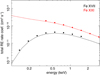 |
Fig. 1. Total resonant excitation (RE) rate coefficients of Fe XVII and Fe XXI through their neighboring ions as a function of energy. The ground states are not included. The solid lines show the present work, and the data points are taken from Gu (2003). |
The current approach enables a level-resolved calculation. In Fig. 2, we plot the n−dependent partial resonances for the different d and f states of Fe XVII excitation. The four lowest excited states, giving the M2 magnetic quadrupole forbidden line (2s22p53s 3P2), the 3G electronic dipole allowed line (2s22p53s 1P1), the M1 magnetic dipole forbidden line (2s22p53s 3P0), and the 3F spin-forbidden intercombination line (2s22p53s 3P1), are highlighted in the plot. The autoionization from 2s22p53lnl′ is the dominant channel to populate the excited states directly, while the contribution from 2s2p64lnl′ is nearly negligible. The low Rydberg states (n ≤ 5) of the doubly excited 2s22p53lnl′ states can autoionize mostly to the ground of Fe XVII, the resonances to excited states thus show a sharp rise at n = 7, and a mild decrease towards higher Rydberg states. For the other d states, the resonances decrease monotonically as a function of n except for a few minor peaks at high-n.
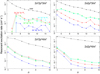 |
Fig. 2. Resonant excitation rate coefficients for Fe XVII at an energy of 0.4 keV as a function of principle quantum number n. The four panels plot the resonances through four main autoionizing Fe XVI states: 2s22p53lnl′, 2s2p63lnl′, 2s22p54lnl′, and 2s2p64lnl′. The autoionization into the lowest four excited states of Fe XVII are highlighted with four different colors. |
As described in Sect. 2, the resonance decrease towards high-n is treated by a n−3 scaling on the Auger rates fitted to the low-n data. Previous laboratory measurements of the high-n satellite lines indicated that the actual n-dependence sometimes deviates from the theoretical scaling (Smith et al. 1996), as the radiative branching ratios would also evolve with the quantum numbers. To assess the uncertainty caused by the n−3 assumption, we extend the calculation of n−resolved excitation rates from n = 15 to n = 30 for the resonances of Fe XVII. As shown in Fig. 3, the actual calculations of the resonance strengths into the four lowly-excited states are compared with the n−3 scaling, which is obtained by fitting the excitation rates of n ≤ 15. Combining the resonances from n = 16 to n = 30, the discrepancies between the data and the scaling are ∼1 − 9 × 10⁻¹⁴ cm3 s−1 for the four states. This error appears to be negligible (< 3%) as the total resonant excitation rates are often several 10−12 cm3 s−1 for these states.
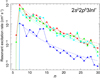 |
Fig. 3. Resonant excitation rate coefficient of the lowest four excited states of Fe XVII through Fe XVI states 2s22p53lnl′ at 0.4 keV, as a function of principle quantum number n up to 30. The dashed lines show the scaling functions for estimating the contribution from the high-n states. |
In Appendix B, we present a systematic comparison of the new calculation with previous results on the excitation rate coefficients of Fe-L. The tests, in particular with those from recent R-matrix calculations, show agreement within typical errors of ∼20% on the main transitions, though the discrepancies on the weaker transitions are much larger. This result agrees with the previous reports (e.g., Fernández-Menchero et al. 2017). Similar conclusions can also be obtained by comparing directly the spectra using the two sets of collisional calculations (Sect. 3.4).
3.2. Dielectronic recombination
As described in Sect. 2.2, the state-selective dielectronic recombination rates are calculated for each isolated channel characterized by the intermediate doubly excited level d. We focus on the d states in which the core electron is excited from n = 2 to n = 3 and 4, and the free electron is captured up to n = 7. The 3lnl′ channels are much more important than the 4lnl′ ones for the DR. Before applying the data in the line formation calculation, we compare the current results with the data published by Badnell et al. (2003), which was calculated using the Breit-Pauli intermediate coupling approach.
As shown in Fig. 4, the two calculations broadly agree upon the total DR rates through 3lnl′ to better than 20%. The differences do not appear to be systematic in the energy range for comparison. The main discrepancies are seen in Fe XXII at ∼0.5 keV and Fe XXIV at > 1 keV, where our DR rates are higher than the Badnell results by ∼15%.
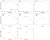 |
Fig. 4. Comparison of total dielectronic recombination rate coefficients. All plots show captures into 3lnl′ states, except for Fe XXIV where the combined 2lnl′ and 3lnl′ are shown. The coefficients include radiative cascades. The large-scale calculations by Badnell et al. (2003) are plotted in red. |
3.3. Level population
Here we evaluate the relative contribution of the various atomic processes to the line formation for a low-density plasma. The level population is calculated using a built-in collisional-radiative program in SPEX, which solves the occupation for each level directly with a large coefficient matrix. To separate different atomic processes, we run the program several times, and in each run we turn on only one of the five processes: direct collisional excitation, resonant excitation, dielectronic recombination, radiative recombination, and innershell ionization. The resonant excitation can be further divided into two components by the autoionizing doubly excited states. The rate coefficients of each process to populate the upper levels of the target lines are recorded independently. All the data used in the line formation are calculated in this work, except for the radiative recombination rates which are based on the calculation in Mao & Kaastra (2016).
It is well known that many relevant levels, in particular those form the forbidden and intercombination lines, are significantly populated by radiative cascades from higher states (Hitomi Collaboration 2018). In Fig. 5, we show the source compositions of the two Fe XVII lines at ∼17 Å. The cascade is clearly the most important component, while the direct contribution is ∼20% of the total rates. Most of the cascades go through the 3s−3p, 3s−3s (1P1−3P0), and 2s−2p transitions. It is therefore important to include the cascade component for each of the atomic processes. As shown in Fig. 6, the cascade-included rate coefficients of each process, for the four 2p53s levels of Fe XVII, are calculated as a function of equilibrium temperature. It can be seen that the direct collisional excitation from the ground state is the dominant process in 0.2 − 1.0 keV, while the indirect excitation contributes ∼30% of the 3P2 population, and ∼10% of the other three states at 0.8 keV. The direct excitation populates these states mainly through cascades from levels at higher energies. The fractional contribution of indirect excitation increases to ∼40 − 50% at 0.2 keV, as the resonant channels become relatively more efficient at a lower energy.
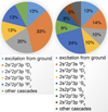 |
Fig. 5. Relative contributions to the formation of Fe XVII 17.09 Å (left) and 17.05 Å (right) lines, from both excitation and radiative cascades. The source levels of cascades are plotted in different colors. |
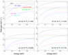 |
Fig. 6. Contributions of rate coefficients to four main Fe XVII lines after the radiative cascades are taken into account, plotted as a function of energy. |
The results of the line formation calculation are recorded in Tables 1 and 2. The levels involved in the new calculation are listed in Table 1. The notation is given in LS-coupling theme. Table 2 lists the temperature-dependent level-resolved rate coefficients for direct collisional excitation, resonant excitation, radiative recombination, and dielectronic recombination. For the excitation, we include the rate coefficients from the ground state, and those from three low-lying excited states. The full tables are available at the CDS.
Levels of the Fe-L ions.
Rate coefficients of the Fe-L in collisional ionization equilibrium.
3.4. Spectra of the Fe-L complex
The model spectrum for each Fe ion obtained from the current calculations is shown in Fig. 7. They are compared with the models based on recent R-matrix collision calculations: Fe XVII from Liang & Badnell (2010), Fe XVIII from Witthoeft et al. (2006), Fe XIX from Butler & Badnell (2008), Fe XX from Witthoeft et al. (2007), Fe XXI from Badnell & Griffin (2001), Fe XXII from Liang et al. (2012), Fe XXIII from Fernández-Menchero et al. (2014), and Fe XXIV from Liang & Badnell (2011). The spectra are smoothed to the resolution of the microcalorimeter onboard Athena (Nandra et al. 2013). The two sets of spectra are calculated using the same rate equation for solving the level population, and the input atomic data are the same except for the collisional excitation. Therefore, the differences can be interpreted as the representative atomic uncertainties due to the theoretical modeling of the collision processes.
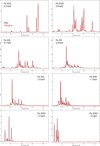 |
Fig. 7. Model spectra of Fe XVII to Fe XXIV in the Fe-L band, obtained from the new FAC (black) and R-matrix (red) calculations. The spectra are smoothed by a Gaussian with σ ≈ 2 eV, similar to the resolution of Athena. The temperature of each spectrum is set to the value of peak ion concentration in equilibrium. |
As shown in Fig. 7, the discrepancies between two codes, at temperatures of peak ion concentration in equilibrium, are mostly within 20% on the main Fe-L transitions. The R-matrix results give slightly higher emissivities for the Fe XVII line at 17 Å and the Fe XX line at 12.8 Å, while the FAC calculation produces a higher Fe XVIII transition at 14.2 Å and a higher Fe XIX line at 13.5 Å. The differences become significantly larger for the weaker transitions of Fe XVIII, Fe XIX, and Fe XX. Similar results can be found in Fernández-Menchero et al. (2017). As for Fe XXI to Fe XXIV, the two calculations agree within a few percent for all the main lines, as well as for most of the weaker ones. This comparison would help us to identify and prioritize the areas where laboratory measurements are needed to distinguish the theoretical models.
Figure 8 illustrates the contributions from different line-formation processes to the model spectrum obtained with the FAC calculation. This is achieved by a partial line formation calculation, including only a subset of atomic data for particular processes. The direct collisional excitation with cascade is found to be dominant, at the temperature of peak ion concentration, for most lines in the Fe-L band. This confirms the results shown in Fig. 6. The cascade from highly excited levels (n ≥ 4) has a moderate contribution. It is especially relevant for several lines, for example, the Fe XVII lines at 16.80 Å, 17.05 Å, and 17.09 Å, the Fe XVIII lines at 15.63 Å, 15.83 Å, and 16.07 Å, the Fe XIX lines at 14.67 Å and 15.08 Å, the Fe XX line at 13.77 Å, the Fe XXI line at 13.25 Å, the Fe XXII line at 12.50 Å, the Fe XXIII lines at 11.02 Å and 11.74 Å, and the Fe XXIV lines at 10.62 Å, 11.03 Å, 11.17 Å, and 11.43 Å.
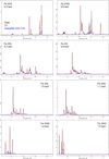 |
Fig. 8. Model spectra of Fe XVII to Fe XXIV in the Fe-L band with the FAC calculation, highlighting the contribution from direct collisional excitation including the cascades (red), and the contribution from the highly excited levels with n > 3 (blue). |
3.5. Comparing with G03
The distorted wave calculation of G03 with the FAC code provided the rate coefficients of direct excitation, resonant excitation, dielectronic recombination, radiative recombination, and innershell processes that populate the n = 2 and n = 3 states, for all the related L-shell species. Fits using the G03 data to the XMM-Newton and Chandra grating spectra of Capella yielded a reasonable agreement (Gu et al. 2006). To justify the updates of our work from G03, here we present a systematic comparison of the two papers.
-
G03 calculated the collisional excitation only from the ground state. As shown in Appendix A and Table 2, we consider both the ground state and the low-lying excited states, as the latter is necessary for modeling intermediate- and high-density plasma.
-
Our calculation is done using the latest version of the FAC code, while G03 was based on an early version. In Fig. 9a, Fe XVII resonant excitation rates for two low-lying levels using the latest code (version 1.1.4) are compared with those calculated with the code version 1.0. The latest version gives lower resonant rates, by ∼5% for the 3s 3P2 level and ∼30% for the 3s 1P1 level, than the early version.
-
As already noted in the Introduction, G03 published the rate coefficients for a complete set of levels with n = 2 and 3 in the paper. This contains the key transitions in the Fe-L complex; however, as shown in Brickhouse et al. (2000), the quantum number n is still too low to sufficiently model the high-resolution spectra from bright X-ray coronal sources. The high-n contributions are crucial for such sources. To allow testing with real observational data (Sect. 4), in this work we calculate all the processes populating the states up to n = 5.
-
The configurations of the doubly excited states (states d in Sect. 2) are slightly different in two calculations. G03 limited their configurations up to l′ ≤ 7 for 3lnl′, and l′ ≤ 4 for 4lnl′, while we include all possible configurations for each n. In principle, the resonant excitation rate coefficients will increase by the additional doubly excited levels. For the two Fe XVII test levels shown in Fig. 9b, the resonant rates using the l−limited calculations are indeed lower, by ∼10 − 15%, than those obtained in the complete calculation. As the l−limited rate coefficients shown in Fig. 9b are obtained with FAC version 1.0, they could be compared directly with the G03 results. It appears that the two sets of rates still differ by 5 − 20%, suggesting that there are other sources of discrepancy in the calculation.
-
According to Eq. (4), the different ionization balance used in the two calculations might introduce discrepancies to the dielectronic recombination rates. To quantify the effect, we apply the ionization balance from G03 and calculate the rates again for the Fe XVII test levels. As shown in Fig. 9c, the rates with the G03 ionization balance are lower by ∼8% than the rates with the balance from Urdampilleta et al. (2017). This is because the Fe XVIII to Fe XVII ratios in the new ionization balance standard are slightly higher than those in G03.
-
G03 calculated the level populations in a hierarchical way. First, a large number of levels were grouped into super levels. The overall population of each super level was calculated. It was then partitioned into each level within the group. In our work, the populations of all levels are solved at once using a large coefficient matrix. As reported in Lucy (2001), the super level method applying to a system with ∼1000 levels can reach an accuracy of 0.1 with 6 iterations, and 0.01 with 20 iterations. Meanwhile, Poirier & de Gaufridy de Dortan (2007) showed that the super level method, as adopted in G03, might become less accurate when the rms deviation of transition rates inside one super level increases.
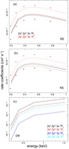 |
Fig. 9. Comparison of the G03 and the present calculations. Panel a: Fe XVII resonant excitation rate coefficients for two low-lying levels, calculated with FAC version 1.1.4 (solid) and version 1.0 (dashed). The G03 results are shown in data points. Panel b: Fe XVII resonant excitation rates of the two levels, obtained with a full calculation with FAC version 1.1.4 (solid) and with a l-limited calculation with FAC version 1.0 (dashed). The latter can be compared directly with the G03 data points. Panel c: Fe XVII dielectronic recombination rates for four low-lying levels obtained with the ionization concentration data of Urdampilleta et al. (2017; solid) and those from G03 (dashed). |
To summarize, we prove that the new theoretical calculation has become both more accurate and more complete than the pioneering G03 calculation.
4. Application to high-resolution X-ray grating data
Here we test the new Fe-L calculations on high-spectral-resolution X-ray data of celestial objects. The targets are selected to be the intracluster medium (ICM) of bright nearby elliptical galaxies and galaxy clusters. They can be regarded as an ideal plasma in collisional ionization equilibrium thermalized to a balance temperature of ∼0.5 − 1.5 keV, and enriched to near-solar abundances (Mernier et al. 2017; Hitomi Collaboration 2017). Although the X-ray fluxes of the ICM sources are substantially lower than those of the coronae of nearby stars (e.g., Capella), they are in general astrophysically simpler, as the temperature components mixed into the ICM emission model are apparently fewer than those of the stellar coronae.
The main purpose of the testing is to reveal the possible biases and systematic uncertainties on the key source parameters due to the change of the underlying atomic database. Three databases with different Fe-L calculations are established. The default data in SPEX version 3.04 are used as the first model (hereafter model 0), which include distorted wave calculations of the direct collisional excitation, and a limited set of dielectronic recombination rates for the Fe-L species (Sect. 2.2). The second model (hereafter model 1) includes a complete set of the new calculations done in this work. We also construct the third model (hereafter model 2) by implementing the recent R-matrix calculations for the collisional excitation (see the list in Sect. 3.4). The atomic structure, radiative recombination, dielectronic recombination, and the innershell data of model 1 and model 2 are the same.
In principle, model 0 should be the least accurate among the three due to the incomplete resonance channels, though it is currently widely used in X-ray astronomy (Hitomi Collaboration 2017, 2018; Ogorzalek et al. 2017; Mernier et al. 2016a,b, 2017; Mao et al. 2019). Model 1 and model 2 should be of similar quality, though they are still different in many places (Fig. 7). Comparing the astronomical measurements using model 0 with the other two will indicate the possible biases in the previous results reported in the literature. The difference between the model 1 and model 2 results can be used as a rough estimate of the representative systematic uncertainties from atomic databases.
Note that the test with the observed data does not verify the new atomic calculation. In fact, none of the current observational data allow a full validation of the atomic database. The astrophysical effects, such as the differential emission measure distribution and the resonant scattering, along with the common assumptions made in analysis (e.g., uniform abundances for all temperature components), might hamper an accurate benchmark of the atomic database. The data from controlled laboratory experiments (Brown et al. 2006) are clearly more suited for such a purpose.
4.1. XMM-Newton grating data
Among the current X-ray observatories, the Reflection Grating Spectrometer (RGS, den Herder et al. 2001) onboard XMM-Newton has the unique power to resolve the Fe-L emission from the ICM into individual lines. The RGS spectra have been used for measuring the chemical abundances of the ellipticals and galaxy clusters (de Plaa et al. 2017), determining the turbulence velocity (de Plaa et al. 2012; Pinto et al. 2015; Ogorzalek et al. 2017), and even probing weak non-thermal charge exchange emission lines (Gu et al. 2018b,a). These measurements are all sensitive to the underlying atomic modeling. Here we apply our new calculation to a sample of RGS data of nearby elliptical galaxies and clusters.
All the testing objects are selected from the CHEmical Evolution RGS Sample (CHEERS), which is made up of 44 representative nearby X-ray bright galaxies and clusters (de Plaa et al. 2017). In this work, we focus on objects showing strong Fe XVII lines in the spectra. The RGS study of Pinto et al. (2016) had the same research focus, leading them to select a subsample of 24 objects. For the 24 objects, we further remove those with data of poor spectral quality. Objects with very diffuse morphology, such as M 87, are not included in the final sample, as their spectra suffer too much from the instrumental broadening. The final sample consists of 15 objects. The properties of the selected targets are listed in Table 3.
XMM-Newton RGS data.
We process the XMM-Newton RGS and MOS data, following the method described in Gu et al. (2018b). The MOS data are used for screening soft proton flares and for deriving the spatial extent of the source along the dispersion direction of the RGS detector.
The Science Analysis System (SAS) v16.1.0 and the latest calibration files (March 2018) are used for data reduction. The time interval contaminated by soft protons is identified using the light curves of the RGS CCD9 and the MOS data. The flaring periods are filtered out by a 2σ clipping. For each object, two source spectra are extracted from a ∼3.4 arcmin-wide belt and a ∼0.8 arcmin-wide belt centered on the emission peak. The modeled background spectra are used in the spectral analysis.
Since RGS is a spectrometer without a slit, the source spatial extent causes the spectral features to be broadened. To model the broadening, we extract the MOS1 image in detector coordinate in 7 − 30 Å, and calculate the surface brightness profile in the RGS dispersion direction. The brightness profiles are convolved with the model spectrum using the SPEX model lpro.
4.2. Spectral modeling
We analyze the first order RGS1 and RGS2 spectra in the 7 − 30 Å band. The metal abundances are scaled to the proto-solar standard of Lodders et al. (2009), and the Galactic absorption column densities are taken from Mernier et al. (2016a). The new ionization balance calculation presented in Urdampilleta et al. (2017) is applied. The best-fit parameters are obtained by minimizing the C-statistics.
The dominant thermal component of the targets is first modeled with a cie component in SPEX. This is sometimes inadequate, as many of the targets show both hot and cool gas phases (Frank et al. 2013). Therefore, we also fit the data with two cie models of different temperatures. Free parameters of the thermal components are the emission measure, the temperature, the abundances of N, O, Ne, Mg, Fe, and Ni, and the velocity of the microturbulence. In the case of two cie, the abundances and the turbulent velocities of the two gas phases are bound to each other. As shown in Fig. 11, the two temperature fits are in general better than the single temperature one. For a few objects, such as NGC 1404 and NGC 3411, the C-statistics differences between the two temperature fits and the single temperature fits are small, as the second thermal component appears to be weak.
4.3. Biases and systematic uncertainties in the abundance measurement
We input model 0, model 1, and model 2 to the SPEX software and create three different versions of cie. For each object, the RGS spectrum is fit independently using the three different cie versions. Figure 10 plots two representative spectra of Abell 3526 and NGC 5813 fit with the three models. The two spectra reveal different ionization states, as the mean temperatures are 0.64 keV and 1.6 keV for NGC 5813 and Abell 3526, respectively. The two-temperature structure is taken into account in the fits. It shows that model 1 and model 2 improve significantly relative to model 0 in the fits for NGC 5813. The Fe XVII lines at 17 Å contribute significantly to the fit improvement, as they are clearly affected by the new resonant excitation and dielectronic recombination data (Fig. 6). The improvements on the fits of Abell 3526 are less apparent. The ratio plots show that the maximum discrepancies of the three models are about 10% on Fe XXIV, Fe XXIII, and Fe XVII lines for Abell 3526, and about 20% on Fe XVII lines for NGC 5813.
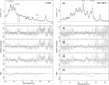 |
Fig. 10. Reflection Grating Spectrometer (RGS) spectra of the central 3.4 arcmin regions of Abell 3526 (left) and NGC 5813 (right) in the 10 − 21 Å band fitted with different models. Panel a: fits by the two-temperature cie with model 1, the residuals are shown in panel b. Panels c and d: residuals of the fits with models 2 and 0, respectively. Panel e: ratios among the three model spectra. The model 0 to model 1 ratios are plotted in blue, and the model 2 to model 1 ratios are plotted in red. It can be seen that the line emissivities of model 1 are higher than those of model 0, but slightly lower than those of model 2, in the 15 − 17 Å band. |
Figure 11 demonstrates that model 1 always gives better fits than model 0. On average, the C-statistic value of the 3.4 arcmin region is improved by 86 (single-temperature) and 64 (two-temperature) for mean degrees of freedom of 713. For the core 0.8 arcmin region, the mean statistics are improved by about 71 (single-temperature) and 44 (two-temperature) for the same degrees of freedom. The resulting ΔC shows a weak dependency on the best-fit temperatures: the fits of the objects with kT ∼ 0.9 − 1.0 keV are less affected by the atomic data update than those with lower or higher temperatures. Model 2 provides a similar improvement on the fit statistics: the average C-statistic values reduce by 84 (single-temperature) and 61 (two-temperature) from the model 0 fits for the 3.4 arcmin region. It is not possible to distinguish between model 1 and model 2 with the current fits.
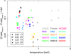 |
Fig. 11. Relative difference of the best-fit C-statistic values with model 1 and model 0 as a function of temperature. The temperatures are obtained using the single-temperature fits with model 1. |
Figures 12 and 13 show a mild bias in temperature and abundance measurement due to the atomic data update. For the single-temperature modeling, the sample-average temperature increases by 2%, and the Fe abundance decreases by 9% by switching from model 0 to model 1. The ratio of O to Fe abundances would increase by a larger mean value of 13%, as the changes in temperature and Fe abundance would affect indirectly the O abundance (even though the atomic data for oxygen ions remain the same). The O/Fe ratio is a key parameter for quantifying the relative enrichment contribution from different types of supernovae to the interstellar and intracluster medium (de Plaa et al. 2017). The biases on the abundances are larger at ≤0.8 keV and potentially also significant at ≥1.3 keV, while the best-fit values around ∼1 keV obtained with the SPEX v3.04 code might require just a minor revision.
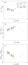 |
Fig. 12. Ratios of the best-fit (panel a) temperatures, (panel b) Fe abundances, and (panel c) O/Fe with model 1 and model 0. All values are obtained in the single-temperature fits. Data with crosses and dots are ratios determined in the 3.4 arcmin and 0.8 arcmin regions, respectively. |
As for the two-temperature astrophysical modeling, the average Fe abundance decreases by 12% with model 1, and the mean O/Fe ratio increases by 16%, relative to that obtained with model 0. These differences are slightly larger than the single-temperature cases. As shown in Fig. 13, the changes in the Fe abundances show very weak dependence on the temperature. The O/Fe ratios still vary with temperature: a higher bias of ∼20% is found at ≤0.8 keV, while the bias at ≥1 keV becomes slightly lower. Considering that the two-temperature model is naturally a better recipe for the cool-core objects than the single-temperature one (Gu et al. 2012), the biases found in the two-temperature fits should be a better approximation to the reality.
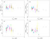 |
Fig. 13. Ratios of the best-fit (panel a) Fe abundances and (panel b) O/Fe with model 1 and model 0, obtained in the two-temperature fits. Panels c and d: ratios of Fe abundances and O/Fe with model 1 and model 2 in the two-temperature fits. The colors are the same as Fig. 12. |
As shown in Fig. 13, the Fe abundances measured with model 2 appear to deviate from the model 1 results. The observed discrepancies seem to change as a function of temperature: the mean Fe abundance with model 1 is higher by ∼10% at 0.7 keV, but it becomes lower by 10% at 1.5 keV than the mean model 2 abundance. Current RGS data cannot decisively distinguish between model 1 and model 2 by the fit statistics, therefore, the 10% abundance differences can be treated as systematic uncertainties. Furthermore, taking into account the model 1 versus model 0 ratios (Fig. 13), the Fe abundances with model 2 are lower than the model 0 values by ∼20% at ∼0.7 keV, while the difference becomes smaller as the temperature increases (or decreases), and largely diminishes at 1.5 keV. The mean O/Fe ratio measured with model 2 is 23% higher than the model 0 value below 1 keV, and the two values converge at 1.5 keV.
The bias in measuring the O/Fe ratio could affect the fraction of type Ia supernovae contributing to the ICM enrichment (see the reviews of Böhringer & Werner 2010 and Mernier et al. 2018). As shown in Simionescu et al. (2009), the increase of 23% in the O/Fe ratio might lead to a lower type Ia fraction by ∼5 − 15%, depending on the supernova explosion mechanism. The improved abundance ratio measurement can, in principle, also better distinguish among the type II supernovae models with different levels of pre-enrichment of the progenitors and with different initial-mass functions (Mernier et al. 2016b).
This experiment provides a general idea of the spectroscopic sensitivity on the new Fe-L atomic calculations, for RGS spectra of a limited sample of elliptical galaxies and cool clusters with temperatures of 0.6 − 1.5 keV. To summarize, for the cool objects (< 1 keV), the Fe abundances measured with the new calculations (model 1 and model 2) are consistently lower by 10%−20% than those derived from the standard plasma code (model 0). The systematic uncertainties on the Fe abundances, determined by comparing the model 1 and model 2 fits, are up to 10% for the current observations.
The test is far from complete, as the new calculations still need to be tested on further cooler (< 0.6 keV) or hotter (> 1.5 keV) objects in CIE, non-equilibrium ionization objects, as well as the objects affected by a strong photon field. On the other hand, the current RGS spectra resolve mostly the main transitions, while the satellite lines, which are strongly affected by the new atomic database, cannot be fully tested. We expect that the new high-resolution X-ray spectrometers on board the X-ray imaging and spectroscopy mission (XRISM, Tashiro et al. 2018) and Athena will be able to provide a sufficient test to these weak lines.
5. Concluding remarks
By carrying out a large-scale theoretical calculation of the electron impact on ions of Fe XVII to Fe XXIV, we present a set of new atomic data for modeling the Fe-L complex. The calculation includes a large set of atomic levels for each ion, allowing full configuration interaction and all kinds of resonant processes. The resonant excitation and the dielectronic recombination are found to affect strongly a significant portion of the major transitions. We present a set of detailed comparisons of the new calculation with available R-matrix results, on both the collisional rates and the model spectra based on the line formation calculations. It shows that the two calculations agree within 20% on most of the main transitions. The comparison will be fed into the prioritization of the future laboratory benchmarks on the Fe-L modeling.
The current SPEX code includes mostly non-resonant atomic calculations. The fact that many previous RGS results on elliptical galaxies and galaxy clusters are based on a non-resonant database is worrying. To assess the possible bias, we apply the new FAC calculation with complete resonances to a RGS sample of 15 cool-core ellipticals and clusters. We find that the Fe abundances measured with the current SPEX v3.04 code are on average biased high by 12%. The O/Fe abundance ratio, which is widely used for assessing the population of the enriching supernovae, is underestimated by a mean value of 16%. Furthermore, the Fe abundances measured with the R-matrix model show discrepancies of ≤ 10% from the values with the FAC model. Current data cannot decisively distinguish between the FAC and the R-matrix models, therefore the 10% abundance difference has to be treated as systematic uncertainties.
To update the atomic database in a plasma code (such as SPEX), it is ideal to take the best from the R-matrix and the FAC calculations. In theory, the accuracy of R-matrix data might be considered superior to that of the FAC calculation. The R-matrix data should be implemented on the low-lying levels, which form the main X-ray transitions. For the high levels, as the R-matrix data gradually becomes sparse, the new FAC calculation with isolated resonances can be implemented as a valid approximation. This would form a recommended database used in most of the analysis. On the other hand, it might be desirable to keep a second database with the new FAC calculations for both the low and high levels. Since the R-matrix and FAC calculations might represent two ends of the theoretical space, comparing the fits with the recommended and the second databases might directly reflect the systematic atomic uncertainties on the source parameters.
The next step in the Fe-L work will be twofold. First, testing with astrophysical objects with existing observatories will be continued. As shown in the test with the RGS data, benchmarks using astrophysical objects require not only a compatible atomic database, but also a proper analysis technique for modeling out the astrophysical effects. Second, we will put forward a dedicated benchmark with ground-based laboratory experiments using electron beam ion trap devices, where plasma in a Maxwellian distribution can be simulated. By checking the consistency between the models and the astrophysical as well as the experimental spectra for each visible Fe-L transition, we will identify the potential areas where the theoretical calculations can be further improved. Some iterations of such work will be needed to ensure that the atomic codes are ready for the future high-resolution X-ray spectra obtained with XRISM and Athena.
http://open.adas.ac.uk, ADF04.
Acknowledgments
L.G. is supported by the RIKEN Special Postdoctoral Researcher Program. SRON is supported financially by NWO, the Netherlands Organization for Scientific Research. A.S. is supported by the Women In Science Excel (WISE) program of the Netherlands Organisation for Scientific Research (NWO), and acknowledges the MEXT World Premier Research Center Initiative (WPI) and the Kavli IPMU for the continued hospitality.
References
- Aggarwal, K. M., & Keenan, F. P. 2013, At. Data Nucl. Data Tables, 99, 156 [NASA ADS] [CrossRef] [Google Scholar]
- Aggarwal, K. M., Keenan, F. P., & Msezane, A. Z. 2003, ApJS, 144, 169 [NASA ADS] [CrossRef] [Google Scholar]
- Audard, M., Behar, E., Güdel, M., et al. 2001, A&A, 365, L329 [NASA ADS] [CrossRef] [EDP Sciences] [Google Scholar]
- Badnell, N. R. 2006, ApJS, 167, 334 [NASA ADS] [CrossRef] [Google Scholar]
- Badnell, N. R., & Griffin, D. C. 2001, J. Phys. B At. Mol. Phys., 34, 681 [NASA ADS] [CrossRef] [Google Scholar]
- Badnell, N. R., Griffin, D. C., Gorczyca, T. W., & Pindzola, M. S. 1994, Phys. Rev. A, 50, 1231 [NASA ADS] [CrossRef] [Google Scholar]
- Badnell, N. R., O’Mullane, M. G., Summers, H. P., et al. 2003, A&A, 406, 1151 [NASA ADS] [CrossRef] [EDP Sciences] [Google Scholar]
- Behar, E., Rasmussen, A. P., Griffiths, R. G., et al. 2001, A&A, 365, L242 [NASA ADS] [CrossRef] [EDP Sciences] [Google Scholar]
- Bernitt, S., Brown, G. V., Rudolph, J. K., et al. 2012, Nature, 492, 225 [NASA ADS] [CrossRef] [Google Scholar]
- Böhringer, H., & Werner, N. 2010, A&ARv, 18, 127 [NASA ADS] [CrossRef] [Google Scholar]
- Brickhouse, N. S., Dupree, A. K., Edgar, R. J., et al. 2000, ApJ, 530, 387 [NASA ADS] [CrossRef] [Google Scholar]
- Brinkman, A. C., Gunsing, C. J. T., Kaastra, J. S., et al. 2000, ApJ, 530, L111 [NASA ADS] [CrossRef] [Google Scholar]
- Brown, G. V. 2008, Can. J. Phys., 86, 199 [NASA ADS] [CrossRef] [Google Scholar]
- Brown, G. V., Beiersdorfer, P., Liedahl, D. A., Widmann, K., & Kahn, S. M. 1998, ApJ, 502, 1015 [NASA ADS] [CrossRef] [Google Scholar]
- Brown, G. V., Beiersdorfer, P., Chen, H., et al. 2006, Phys. Rev. Lett., 96, 253201 [NASA ADS] [CrossRef] [PubMed] [Google Scholar]
- Butler, K., & Badnell, N. R. 2008, A&A, 489, 1369 [NASA ADS] [CrossRef] [EDP Sciences] [Google Scholar]
- Chen, G. X., & Pradhan, A. K. 2002, Phys. Rev. Lett., 89, 013202 [NASA ADS] [CrossRef] [Google Scholar]
- Chen, M. H., & Reed, K. J. 1989, Phys. Rev. A, 40, 2292 [NASA ADS] [CrossRef] [Google Scholar]
- Churazov, E., Zhuravleva, I., Sazonov, S., & Sunyaev, R. 2010, Space Sci. Rev., 157, 193 [NASA ADS] [CrossRef] [Google Scholar]
- Cox, D. P., & Tucker, W. H. 1969, ApJ, 157, 1157 [NASA ADS] [CrossRef] [Google Scholar]
- de Plaa, J., Zhuravleva, I., Werner, N., et al. 2012, A&A, 539, A34 [NASA ADS] [CrossRef] [EDP Sciences] [Google Scholar]
- de Plaa, J., Kaastra, J. S., Werner, N., et al. 2017, A&A, 607, A98 [NASA ADS] [CrossRef] [EDP Sciences] [Google Scholar]
- Del Zanna, G. 2006a, A&A, 459, 307 [NASA ADS] [CrossRef] [EDP Sciences] [Google Scholar]
- Del Zanna, G. 2006b, A&A, 447, 761 [NASA ADS] [CrossRef] [EDP Sciences] [Google Scholar]
- Del Zanna, G. 2011, A&A, 536, A59 [NASA ADS] [CrossRef] [EDP Sciences] [Google Scholar]
- Del Zanna, G., Chidichimo, M. C., & Mason, H. E. 2005, A&A, 432, 1137 [NASA ADS] [CrossRef] [EDP Sciences] [Google Scholar]
- Del Zanna, G., Dere, K. P., Young, P. R., Landi, E., & Mason, H. E. 2015, A&A, 582, A56 [NASA ADS] [CrossRef] [EDP Sciences] [Google Scholar]
- den Herder, J. W., Brinkman, A. C., Kahn, S. M., et al. 2001, A&A, 365, L7 [NASA ADS] [CrossRef] [EDP Sciences] [Google Scholar]
- Dere, K. P., Landi, E., Mason, H. E., Monsignori Fossi, B. C., & Young, P. R. 1997, A&AS, 125, 149 [NASA ADS] [CrossRef] [EDP Sciences] [Google Scholar]
- Doron, R., & Behar, E. 2002, ApJ, 574, 518 [NASA ADS] [CrossRef] [Google Scholar]
- Feldman, U. 1995, Mol. Phys., 31, 11 [Google Scholar]
- Fernández-Menchero, L., Del Zanna, G., & Badnell, N. R. 2014, A&A, 566, A104 [NASA ADS] [CrossRef] [EDP Sciences] [Google Scholar]
- Fernández-Menchero, L., Zatsarinny, O., & Bartschat, K. 2017, J. Phys. B At. Mol. Phys., 50, 065203 [NASA ADS] [CrossRef] [Google Scholar]
- Foster, A. R., Ji, L., Smith, R. K., & Brickhouse, N. S. 2012, ApJ, 756, 128 [NASA ADS] [CrossRef] [Google Scholar]
- Frank, K. A., Peterson, J. R., Andersson, K., Fabian, A. C., & Sanders, J. S. 2013, ApJ, 764, 46 [NASA ADS] [CrossRef] [Google Scholar]
- Gilfanov, M. R., Syunyaev, R. A., & Churazov, E. M. 1987, Sov. Astron. Lett., 13, 3 [NASA ADS] [Google Scholar]
- Goldstein, W. H., Osterheld, A., Oreg, J., & Bar-Shalom, A. 1989, ApJ, 344, L37 [NASA ADS] [CrossRef] [Google Scholar]
- Gu, M. F. 2003, ApJ, 582, 1241 [NASA ADS] [CrossRef] [Google Scholar]
- Gu, M. F. 2008, Can. J. Phys., 86, 675 [NASA ADS] [CrossRef] [Google Scholar]
- Gu, M. F., Gupta, R., Peterson, J. R., Sako, M., & Kahn, S. M. 2006, ApJ, 649, 979 [NASA ADS] [CrossRef] [Google Scholar]
- Gu, L., Xu, H., Gu, J., et al. 2012, ApJ, 749, 186 [NASA ADS] [CrossRef] [Google Scholar]
- Gu, L., Zhuravleva, I., Churazov, E., et al. 2018a, Space Sci. Rev., 214, 108 [NASA ADS] [CrossRef] [Google Scholar]
- Gu, L., Mao, J., de Plaa, J., et al. 2018b, A&A, 611, A26 [NASA ADS] [CrossRef] [EDP Sciences] [Google Scholar]
- Hitomi Collaboration (Aharonian, F., et al.) 2017, Nature, 551, 478 [NASA ADS] [CrossRef] [Google Scholar]
- Hitomi Collaboration (Aharonian, F., et al.) 2018, PASJ, 70, 12 [NASA ADS] [Google Scholar]
- Jones, C., & Forman, W. 1984, ApJ, 276, 38 [NASA ADS] [CrossRef] [Google Scholar]
- Kaastra, J. S. 1992, Internal SRON-Leiden Report [Google Scholar]
- Kaastra, J. S., Mewe, R., & Nieuwenhuijzen, H. 1996, in UV and X-ray Spectroscopy of Astrophysical and Laboratory Plasmas, eds. K. Yamashita, & T. Watanabe, 411 [Google Scholar]
- Landini, M., & Monsignori Fossi, B. C. 1972, A&AS, 7, 291 [NASA ADS] [Google Scholar]
- Liang, G. Y., & Badnell, N. R. 2010, A&A, 518, A64 [NASA ADS] [CrossRef] [EDP Sciences] [Google Scholar]
- Liang, G. Y., & Badnell, N. R. 2011, A&A, 528, A69 [NASA ADS] [CrossRef] [EDP Sciences] [Google Scholar]
- Liang, G. Y., Badnell, N. R., & Zhao, G. 2012, A&A, 547, A87 [NASA ADS] [CrossRef] [EDP Sciences] [Google Scholar]
- Loch, S. D., Pindzola, M. S., Ballance, C. P., & Griffin, D. C. 2006, J. Phys. B At. Mol. Phys., 39, 85 [Google Scholar]
- Lodders, K., Palme, H., & Gail, H. P. 2009, in Landolt- Börnstein, New Series, Chap. 4.4, ed. J. E. Trümper (Berlin, Heidelberg, New York: Springer-Verlag), VI/4B, 560 [Google Scholar]
- Lucy, L. B. 2001, MNRAS, 326, 95 [NASA ADS] [CrossRef] [Google Scholar]
- Mao, J., & Kaastra, J. 2016, A&A, 587, A84 [NASA ADS] [CrossRef] [EDP Sciences] [Google Scholar]
- Mao, J., Kaastra, J. S., Mehdipour, M., et al. 2017, A&A, 607, A100 [NASA ADS] [CrossRef] [EDP Sciences] [Google Scholar]
- Mao, J., de Plaa, J., Kaastra, J. S., et al. 2019, A&A, 621, A9 [NASA ADS] [CrossRef] [EDP Sciences] [Google Scholar]
- Mernier, F., de Plaa, J., Pinto, C., et al. 2016a, A&A, 592, A157 [NASA ADS] [CrossRef] [EDP Sciences] [Google Scholar]
- Mernier, F., de Plaa, J., Pinto, C., et al. 2016b, A&A, 595, A126 [NASA ADS] [CrossRef] [EDP Sciences] [Google Scholar]
- Mernier, F., de Plaa, J., Kaastra, J. S., et al. 2017, A&A, 603, A80 [NASA ADS] [CrossRef] [EDP Sciences] [Google Scholar]
- Mernier, F., Biffi, V., Yamaguchi, H., et al. 2018, Space Sci. Rev., 214, 129 [NASA ADS] [CrossRef] [Google Scholar]
- Mewe, R. 1972a, Sol. Phys., 22, 459 [NASA ADS] [CrossRef] [Google Scholar]
- Mewe, R. 1972b, A&A, 20, 215 [NASA ADS] [Google Scholar]
- Nandra, K., Barret, D., & Barcons, X. 2013, ArXiv e-prints [arXiv:1306.2307] [Google Scholar]
- Ogorzalek, A., Zhuravleva, I., Allen, S. W., et al. 2017, MNRAS, 472, 1659 [NASA ADS] [CrossRef] [Google Scholar]
- Phillips, K. J. H., Bhatia, A. K., Mason, H. E., & Zarro, D. M. 1996, ApJ, 466, 549 [NASA ADS] [CrossRef] [Google Scholar]
- Pinto, C., Sanders, J. S., Werner, N., et al. 2015, A&A, 575, A38 [NASA ADS] [CrossRef] [EDP Sciences] [Google Scholar]
- Pinto, C., Fabian, A. C., Ogorzalek, A., et al. 2016, MNRAS, 461, 2077 [NASA ADS] [CrossRef] [Google Scholar]
- Poirier, M., & de Gaufridy de Dortan, F. 2007, J. Appl. Phys., 101, 063308 [NASA ADS] [CrossRef] [Google Scholar]
- Raymond, J. C., & Smith, B. W. 1977, ApJS, 35, 419 [NASA ADS] [CrossRef] [Google Scholar]
- Shah, C., Crespo López-Urrutia, J. R., Gu, M. F., et al. 2019, ApJ, accepted [arXiv:1903.04506] [Google Scholar]
- Simionescu, A., Werner, N., Böhringer, H., et al. 2009, A&A, 493, 409 [NASA ADS] [CrossRef] [EDP Sciences] [Google Scholar]
- Smith, B. W., Mann, J. B., Cowan, R. D., & Raymond, J. C. 1985, ApJ, 298, 898 [NASA ADS] [CrossRef] [Google Scholar]
- Smith, A. J., Beiersdorfer, P., Decaux, V., et al. 1996, Phys. Rev. A, 54, 462 [NASA ADS] [CrossRef] [Google Scholar]
- Smith, R. K., Brickhouse, N. S., Liedahl, D. A., & Raymond, J. C. 2001, ApJ, 556, L91 [NASA ADS] [CrossRef] [Google Scholar]
- Tashiro, M., Maejima, H., Toda, K., et al. 2018, SPIE Conf. Ser., 10699, 1069922 [Google Scholar]
- Urdampilleta, I., Kaastra, J. S., & Mehdipour, M. 2017, A&A, 601, A85 [NASA ADS] [CrossRef] [EDP Sciences] [Google Scholar]
- Werner, N., Böhringer, H., Kaastra, J. S., et al. 2006, A&A, 459, 353 [NASA ADS] [CrossRef] [EDP Sciences] [Google Scholar]
- Witthoeft, M. C., Badnell, N. R., del Zanna, G., Berrington, K. A., & Pelan, J. C. 2006, A&A, 446, 361 [NASA ADS] [CrossRef] [EDP Sciences] [Google Scholar]
- Witthoeft, M. C., Del Zanna, G., & Badnell, N. R. 2007, A&A, 466, 763 [NASA ADS] [CrossRef] [EDP Sciences] [Google Scholar]
- Xu, H., Kahn, S. M., Peterson, J. R., et al. 2002, ApJ, 579, 600 [NASA ADS] [CrossRef] [Google Scholar]
Appendix A: Density effects
For a low-density plasma, excited levels are quickly depleted by spontaneous cascade, so that only the ground state is significantly populated. At a high electron density, the cascade might be interrupted by collision with electrons. Some of the low-lying levels become thus populated. As a result, the population of the ground state decreases, and the related spectral features, for example, lines from ground excitation, become weaker. On the other side, the transitions from the excited states become substantially more important (Mao et al. 2017).
Figure A.1 illustrates the density-dependent population of several low-lying excited levels for the C-like, B-like, and Be-like Fe. The calculation is done with SPEX, which incorporates the new atomic data obtained in this work. For an electron density lower than 1010 cm−3, the occupations of these levels are negligible, except for the metastable 2s2p 3P0 level, which is populated even at low density due to the narrow de-excitation channel. For the selected low-lying levels shown in the figure, the population rises as the density increases from 1012 cm−3 to 1014 cm−3. At a higher density, the relative level population evolves towards the standard Boltzman distribution, as the excited states would eventually be in a collisional local thermodynamic equilibrium (LTE).
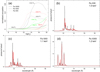 |
Fig. A.1. Density effects on C-like, B-like, and Be-like Fe. Panel a: normalized population of the three low-lying excited levels of C-like, B-like, and Be-like Fe, as a function of electron density. The population of the ground states is not plotted. The density effect on the model spectra for the C-like, B-like, and Be-like Fe is shown in panels b, c, and d, respectively. The spectra of low density (1 cm−3) and intermediate density (1014 cm−3) are plotted in black and red. The temperatures are the same as in Fig. 7. |
The same exercise has been done for the other Fe-L species. For the astrophysical coronal and nebular (< 1014 cm−3) plasma, the density effect is most significant at the three low-lying excited levels for the Fe-L. For the three levels, we calculate the transition rates of direct excitation, resonant excitation, and dielectronic recombination, in a same way as those from the ground states (Sect. 2).
It should be noted that there could be more metastable levels above the three low-lying levels included in the current calculation. Badnell (2006) included six low-lying excited levels for O-like Fe and Be-like Fe, eight for N-like and B-like, and 12 for C-like, as the metastable parent levels used in the radiative recombination calculation. The extra metastable levels would become sensitive at higher density (> 1014 cm−3). We plan to include all the metastable levels in a follow-up calculation.
Figure A.1 shows the model spectra based on the above data, for the C-like, B-like, and Be-like Fe at a low density and an intermediate density of 1014 cm−3. The temperature is set to the value of peak ion concentration in equilibrium. It can be seen that the dominant lines of these ions become weaker at high density, probably because these lines originate from the excitation of the ground states, which have a decreasing population at high density. Some of the satellite lines become stronger, as the low-lying levels contribute significantly to the formation of these lines.
Appendix B: Resonant excitation: consistency check with previous results
Following Sect. 3.1, we compare the electron-impact collision data obtained from the current FAC calculation with those from previous distorted wave and R-matrix works.
B.1. Comparing with classic Fe XVII resonance calculations
In Table B.1, the resonance rates of the Fe XVII ion from the present work are compared with the results in the literature. The values from Smith et al. (1985), Goldstein et al. (1989), Chen & Reed (1989), and Chen & Pradhan (2002) are based on the semirelativistic Hartree-Fock method, a relativistic parametric potential method, the multiconfiguration Dirac-Fock approach, and a Breit-Pauli R-matrix method with a 89-level expansion, respectively. The rate coefficients reported in Smith et al. (1985) are apparently higher than the others. Chen & Reed (1989) suggested that this is partially explained by the incomplete autoionization channels included in Smith et al. (1985). The present calculation gives higher rates than the those of Goldstein et al. (1989) and Chen & Reed (1989) using a similar technique, but lower than the Breit-Pauli R-matrix results. The discrepancies between the Chen & Pradhan (2002) values and our results at 0.2 keV are 42% on the partial rate to 2s22p53s 3P1, and 28% on the total rate.
Partial resonance rates for the 2p53s levels of Fe XVII.
B.2. Comparing with recent R-matrix results: Main transitions
More recently, new R-matrix calculations of Ne-like species were performed by Loch et al. (2006) and Liang & Badnell (2010). The new calculations include more close-coupling expansions than the earlier Breit-Pauli work by Chen & Pradhan (2002). For Fe XVII, the total atomic levels are 139 levels in Loch et al. (2006) and 209 levels in Liang & Badnell (2010). Here we further compare our calculation with the two new results for the four 3s levels of Fe XVII. The effective collision strengths are taken from the OPEN-ADAS database1.
As shown in Fig. B.1, the differences between the three datasets are reasonably small. Our calculation agrees with the R-matrix results within ∼5% for the 3P2 level in 0.1 − 1.0 keV, and within 5 − 20% for the 3P0 level. For the 1P1 and 3P1 levels, our results are slightly lower, by 3 − 10% than those of Liang & Badnell (2010) and 15 − 20% than those of Loch et al. (2006). In general, the differences observed between the FAC and the recent R-matrix calculations are well within the uncertainties among different R-matrix results. The agreement on the Ne-like lines is even better than those on the H-like and He-like species as reported in Hitomi Collaboration (2018).
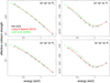 |
Fig. B.1. Maxwellian-averaged collision strengths for four main Fe XVII transitions. Red and green curves are the R-matrix data taken from Liang & Badnell (2010) and Loch et al. (2006). |
The resonance and direct excitation of n = 3 and 4 for Fe XVIII was calculated by Witthoeft et al. (2006), using R-matrix with 195 levels. As shown in Fig. B.2, we compare the calculations of two 3s levels that produce the strong 16 Å line. The FAC and R-matrix results again agree within 10%, which might potentially be ascribed to the uncertainties of the atomic structure for this nine-electron system.
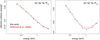 |
Fig. B.2. Same as Fig. B.1 but for two Fe XVIII lines. The R-matrix data from Witthoeft et al. (2006) are shown in red. |
A similar R-matrix tool was used to calculate the electron collisional data for transitions among 342 levels of Fe XIX (Butler & Badnell 2008). As shown in Fig. B.3, we compare the calculations of four key excited levels with n = 3. For the 3s level, the FAC value is higher than the R-matrix one by 20% at 0.2 keV, and by 13% at 1 keV. As for the 3p and 3d levels, the two theoretical models seem to agree within 10% in the temperature range of astrophysical interest.
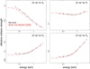 |
Fig. B.3. Same as Fig. B.1 but for four Fe XIX lines. The R-matrix data from Butler & Badnell (2008) are shown in red. |
The electron collision strengths for a total of 302 close-coupling levels of Fe XX were reported in Witthoeft et al. (2007), based on the R-matrix theory using an intermediate-coupling frame transformation method. Their results are compared with the FAC calculation, for four low-lying levels shown in Fig. B.4. The comparison on the 3s 4P5/2 level reveals a maximum discrepancy of ∼20% at 0.4 keV. For the other three levels, the differences between the two datasets are reasonably small.
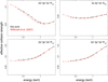 |
Fig. B.4. Same as Fig. B.1 but for four Fe XX lines. The R-matrix data from Witthoeft et al. (2007) are shown in red. |
An R-matrix calculation for C-like Fe excitation was reported by Badnell & Griffin (2001). It was carried out with the intermediate coupling frame transformation method for 200 close-coupling levels. In Fig. B.5, we show collision strengths for four representative levels, which are among the upper levels that produce the brightest emission lines. Our calculation suggests that these levels are significantly contributing to the resonant excitation. The FAC and R-matrix results accord well within < 10% for Te = 0.1 − 10 keV.
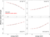 |
Fig. B.5. Same as Fig. B.1 but for four Fe XXI lines. The R-matrix data from Badnell & Griffin (2001) are plotted in red. |
We further test the electron-impact excitation of Fe XXII with the 204-level R-matrix results reported in Liang et al. (2012). As plotted in Fig. B.6, detailed comparisons for the effective collision strengths are made for four representative levels, which are selected again based on the related line emissivities and the resonance contribution. For 2s22p 2P3/2 and 2s23s 2S1/2, the two calculations in general agree for high temperatures, while the FAC values are lower than the R-matrix values by ∼20% at ≤1 keV. The two approaches converge well for the other two levels 2s2p22P1/2 and 2s23d 2D3/2.
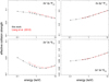 |
Fig. B.6. Same as Fig. B.1 but for four Fe XXII lines. The R-matrix data from Liang et al. (2012) are plotted in red. |
The R-matrix calculation of electron-impact excitation of Fe XXIII was made by Fernández-Menchero et al. (2014), based on 238 fine-structure levels in both the configuration interaction target and close-coupling collision expansions. We compare the collision strengths for four strong Fe XXIII lines with their calculations, on which the resonance has a large effect. As shown in Fig. B.7, the two sets of data agree very well within a difference of ≤5% for Te = 0.1 − 10 keV.
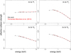 |
Fig. B.7. Same as Fig. B.1 but for four Fe XXIII lines. The R-matrix data from Fernández-Menchero et al. (2014) are shown in red. |
In Fig. B.8 we compare our calculations of the total excitation of four main Fe XXIV lines with the R-matrix results reported in Liang & Badnell (2011). The R-matrix work was done with the intermediate coupling frame transformation method for 195 levels, and the Auger- as well as radiation-damping effects were both taken into account. For 3s 2S1/2, 3d 2D3/2, and 3d 2D5/2, the R-matrix and our data agree well with ∼5%, while for 3p 2P3/2, the difference between the two approaches becomes slightly larger, ∼10%, for the collision strengths at energy of ≤1 keV.
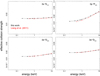 |
Fig. B.8. Same as Fig. B.1 but for four Fe XXIV lines. The R-matrix data from Liang & Badnell (2011) are plotted in red. |
The illustrative comparison indicates that the difference between the modern large-scale isolated resonance calculation and the recent interacting R-matrix becomes now smaller than previously reported in Badnell et al. (1994). The two methods are well within 20% for the direct transitions from the ground states to a few selected excited levels at n = 3. As shown in Fig. 6, some excited levels are heavily populated through cascade, indicating that the line intensities could actually be significantly affected by the excitation rate coefficients to higher states. In the following section, we will give an extensive comparison for all the relevant rates.
B.3. Comparing with recent R-matrix results: Scatter plots
The scatter plot in Fig. B.9 shows the comparison of the effective collision strengths from the current and R-matrix calculations, for all the excitations from the ground states. The R-matrix results are a collection of the works mentioned in Appendix B.2. The plot confirms that the two methods agree on the strongest transitions within uncertainties of ∼20%. However, the discrepancies between the two methods on the weaker transitions are substantially larger, up to a factor of two for Fe XVII and Fe XXIV, and one order of magnitude for the rest ions, at the lowest effective collision strengths. We note that orders of magnitude difference for weak transitions are also found among different R-matrix calculations (intermediate coupling frame transformation, Breit-Pauli, Dirac atomic R-matrix code, Fernández-Menchero et al. 2017 and references therein). These weak transitions would affect the satellite lines directly, and might also influence the main spectral lines collectively through cascade. As shown in Fig. 7, the differences in the main transitions and in the weak transitions are clearly reflected in the model spectra, indicating that both contribute systematic uncertainties that would significantly affect the astrophysical spectral measurements.
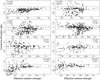 |
Fig. B.9. Ratios of the effective collision strengths from the current calculations to those from the recent R-matrix calculations, for all excitations from the ground states of the Fe-L species. The comparison is made at the temperature with peak ionization concentration of each ion (see Fig. 7). The horizontal lines indicate 20% differences. |
All Tables
All Figures
|
Fig. 1. Total resonant excitation (RE) rate coefficients of Fe XVII and Fe XXI through their neighboring ions as a function of energy. The ground states are not included. The solid lines show the present work, and the data points are taken from Gu (2003). |
| In the text | |
|
Fig. 2. Resonant excitation rate coefficients for Fe XVII at an energy of 0.4 keV as a function of principle quantum number n. The four panels plot the resonances through four main autoionizing Fe XVI states: 2s22p53lnl′, 2s2p63lnl′, 2s22p54lnl′, and 2s2p64lnl′. The autoionization into the lowest four excited states of Fe XVII are highlighted with four different colors. |
| In the text | |
|
Fig. 3. Resonant excitation rate coefficient of the lowest four excited states of Fe XVII through Fe XVI states 2s22p53lnl′ at 0.4 keV, as a function of principle quantum number n up to 30. The dashed lines show the scaling functions for estimating the contribution from the high-n states. |
| In the text | |
|
Fig. 4. Comparison of total dielectronic recombination rate coefficients. All plots show captures into 3lnl′ states, except for Fe XXIV where the combined 2lnl′ and 3lnl′ are shown. The coefficients include radiative cascades. The large-scale calculations by Badnell et al. (2003) are plotted in red. |
| In the text | |
|
Fig. 5. Relative contributions to the formation of Fe XVII 17.09 Å (left) and 17.05 Å (right) lines, from both excitation and radiative cascades. The source levels of cascades are plotted in different colors. |
| In the text | |
|
Fig. 6. Contributions of rate coefficients to four main Fe XVII lines after the radiative cascades are taken into account, plotted as a function of energy. |
| In the text | |
|
Fig. 7. Model spectra of Fe XVII to Fe XXIV in the Fe-L band, obtained from the new FAC (black) and R-matrix (red) calculations. The spectra are smoothed by a Gaussian with σ ≈ 2 eV, similar to the resolution of Athena. The temperature of each spectrum is set to the value of peak ion concentration in equilibrium. |
| In the text | |
|
Fig. 8. Model spectra of Fe XVII to Fe XXIV in the Fe-L band with the FAC calculation, highlighting the contribution from direct collisional excitation including the cascades (red), and the contribution from the highly excited levels with n > 3 (blue). |
| In the text | |
|
Fig. 9. Comparison of the G03 and the present calculations. Panel a: Fe XVII resonant excitation rate coefficients for two low-lying levels, calculated with FAC version 1.1.4 (solid) and version 1.0 (dashed). The G03 results are shown in data points. Panel b: Fe XVII resonant excitation rates of the two levels, obtained with a full calculation with FAC version 1.1.4 (solid) and with a l-limited calculation with FAC version 1.0 (dashed). The latter can be compared directly with the G03 data points. Panel c: Fe XVII dielectronic recombination rates for four low-lying levels obtained with the ionization concentration data of Urdampilleta et al. (2017; solid) and those from G03 (dashed). |
| In the text | |
|
Fig. 10. Reflection Grating Spectrometer (RGS) spectra of the central 3.4 arcmin regions of Abell 3526 (left) and NGC 5813 (right) in the 10 − 21 Å band fitted with different models. Panel a: fits by the two-temperature cie with model 1, the residuals are shown in panel b. Panels c and d: residuals of the fits with models 2 and 0, respectively. Panel e: ratios among the three model spectra. The model 0 to model 1 ratios are plotted in blue, and the model 2 to model 1 ratios are plotted in red. It can be seen that the line emissivities of model 1 are higher than those of model 0, but slightly lower than those of model 2, in the 15 − 17 Å band. |
| In the text | |
|
Fig. 11. Relative difference of the best-fit C-statistic values with model 1 and model 0 as a function of temperature. The temperatures are obtained using the single-temperature fits with model 1. |
| In the text | |
|
Fig. 12. Ratios of the best-fit (panel a) temperatures, (panel b) Fe abundances, and (panel c) O/Fe with model 1 and model 0. All values are obtained in the single-temperature fits. Data with crosses and dots are ratios determined in the 3.4 arcmin and 0.8 arcmin regions, respectively. |
| In the text | |
|
Fig. 13. Ratios of the best-fit (panel a) Fe abundances and (panel b) O/Fe with model 1 and model 0, obtained in the two-temperature fits. Panels c and d: ratios of Fe abundances and O/Fe with model 1 and model 2 in the two-temperature fits. The colors are the same as Fig. 12. |
| In the text | |
|
Fig. A.1. Density effects on C-like, B-like, and Be-like Fe. Panel a: normalized population of the three low-lying excited levels of C-like, B-like, and Be-like Fe, as a function of electron density. The population of the ground states is not plotted. The density effect on the model spectra for the C-like, B-like, and Be-like Fe is shown in panels b, c, and d, respectively. The spectra of low density (1 cm−3) and intermediate density (1014 cm−3) are plotted in black and red. The temperatures are the same as in Fig. 7. |
| In the text | |
|
Fig. B.1. Maxwellian-averaged collision strengths for four main Fe XVII transitions. Red and green curves are the R-matrix data taken from Liang & Badnell (2010) and Loch et al. (2006). |
| In the text | |
|
Fig. B.2. Same as Fig. B.1 but for two Fe XVIII lines. The R-matrix data from Witthoeft et al. (2006) are shown in red. |
| In the text | |
|
Fig. B.3. Same as Fig. B.1 but for four Fe XIX lines. The R-matrix data from Butler & Badnell (2008) are shown in red. |
| In the text | |
|
Fig. B.4. Same as Fig. B.1 but for four Fe XX lines. The R-matrix data from Witthoeft et al. (2007) are shown in red. |
| In the text | |
|
Fig. B.5. Same as Fig. B.1 but for four Fe XXI lines. The R-matrix data from Badnell & Griffin (2001) are plotted in red. |
| In the text | |
|
Fig. B.6. Same as Fig. B.1 but for four Fe XXII lines. The R-matrix data from Liang et al. (2012) are plotted in red. |
| In the text | |
|
Fig. B.7. Same as Fig. B.1 but for four Fe XXIII lines. The R-matrix data from Fernández-Menchero et al. (2014) are shown in red. |
| In the text | |
|
Fig. B.8. Same as Fig. B.1 but for four Fe XXIV lines. The R-matrix data from Liang & Badnell (2011) are plotted in red. |
| In the text | |
|
Fig. B.9. Ratios of the effective collision strengths from the current calculations to those from the recent R-matrix calculations, for all excitations from the ground states of the Fe-L species. The comparison is made at the temperature with peak ionization concentration of each ion (see Fig. 7). The horizontal lines indicate 20% differences. |
| In the text | |
Current usage metrics show cumulative count of Article Views (full-text article views including HTML views, PDF and ePub downloads, according to the available data) and Abstracts Views on Vision4Press platform.
Data correspond to usage on the plateform after 2015. The current usage metrics is available 48-96 hours after online publication and is updated daily on week days.
Initial download of the metrics may take a while.