| Issue |
A&A
Volume 626, June 2019
|
|
|---|---|---|
| Article Number | A19 | |
| Number of page(s) | 6 | |
| Section | Stellar structure and evolution | |
| DOI | https://doi.org/10.1051/0004-6361/201935412 | |
| Published online | 05 June 2019 | |
Long X-ray flares from the central source in RCW 103
XMM-Newton and VLT observations in the aftermath of the 2016 outburst
1
INAF–Istituto di Astrofisica Spaziale e Fisica Cosmica di Milano, Via A. Corti 12, 20133 Milano, Italy
e-mail: This email address is being protected from spambots. You need JavaScript enabled to view it.
2
INFN–Istituto Nazionale di Fisica Nucleare, Sezione di Pavia, Via A. Bassi 6, 27100 Pavia, Italy
3
Dipartimento di Fisica e Astronomia “Galileo Galilei”, Università di Padova, Via F. Marzolo 8, 35131 Padova, Italy
4
Mullard Space Science Laboratory, University College London, Holmbury St. Mary, Dorking, Surrey RH5 6NT, UK
5
Institute of Space Sciences (ICE, CSIC), Campus UAB, Carrer de Can Magrans s/n, 08193 Barcelona, Spain
6
Institut d’Estudis Espacials de Catalunya (IEEC), Gran Capità 2–4, 08034 Barcelona, Spain
7
European Southern Observatory, Karl-Schwarzschild-Straße 2, 85748 Garching bei München, Germany
8
Scuola Universitaria Superiore IUSS Pavia, Piazza della Vittoria 15, 27100 Pavia, Italy
9
INAF–Osservatorio Astronomico di Roma, Via Frascati 33, 00078 Monteporzio Catone, Italy
10
Janusz Gil Institute of Astronomy, University of Zielona Góra, ul. Szafrana 2, 65-516 Zielona Góra, Poland
11
Anton Pannekoek Institute for Astronomy, University of Amsterdam, Science Park 904, 1098 XH Amsterdam, The Netherlands
Received:
6
March
2019
Accepted:
10
April
2019
Abstract
We observed the slowly revolving pulsar 1E 161348–5055 (1E 1613, spin period of 6.67 h) in the supernova remnant RCW 103 twice with XMM-Newton and once with the Very Large Telescope (VLT). The VLT observation was performed on 2016 June 30, about a week after the detection of a large outburst from 1E 1613. At the position of 1E 1613, we found a near-infrared source with Ks = 20.68 ± 0.12 mag that was not detected (Ks > 21.2 mag) in data collected with the same instruments in 2006, during X-ray quiescence. Its position and behavior are consistent with a counterpart in the literature that was discovered with the Hubble Space Telescope in the following weeks in adjacent near-IR bands. The XMM-Newton pointings were carried out on 2016 August 19 and on 2018 February 14. While the collected spectra are similar in shape between each other and to what is observed in quiescence (a blackbody with kT ∼ 0.5 keV plus a second, harder component, either another hotter blackbody with kT ∼ 1.2 keV or a power law with photon index Γ ∼ 3), the two pointings caught 1E 1613 at different luminosity throughout its decay pattern: about 4.8 × 1034 erg s−1 in 2016 and 1.2 × 1034 erg s−1 in 2018 (0.5–10 keV, for the double-blackbody model and for 3.3 kpc), which is still almost about ten times brighter than the quiescent level. The pulse profile displayed dramatic changes, apparently evolving from the complex multi-peak morphology observed in high-luminosity states to the more sinusoidal form characteristic of latency. The inspection of the X-ray light curves revealed two flares with unusual properties in the 2016 observation: they are long (∼1 ks to be compared with 0.1–1 s of typical magnetar bursts) and faint (≈1034 erg s−1, with respect to 1038 erg s−1 or more in magnetars). Their spectra are comparatively soft and resemble the hotter thermal component of the persistent emission. If the flares and the latter component have a common origin, this may be a spot on the star surface that is heated by back-flowing currents that are induced by a magnetospheric twist. In this hypothesis, since the increase in luminosity of 1E 1613 during the flare is only ∼20%, an irregular variation of the same order in the twist angle could account for it.
Key words: X-rays: individuals: 1E 161348–5055 / stars: neutron
© ESO 2019
1. Introduction
The X-ray source 1E 161348–5055 (1E 1613) lies at the center of the young (2 kyr) supernova remnant (SNR) RCW 103. It was discovered with Einstein and was suggested to be a radio-quiet isolated neutron star (NS) by Tuohy & Garmire (1980). Over the years, the behavior of 1E 1613 has set it apart from any other compact object source (De Luca 2008, 2017): the source displays a strong variability on scales of months or years (a large outburst with an increase in luminosity from ∼3 × 1033 to over 3 × 1035 erg s−1 occurred in 1999), and features a modulation in flux with a period of 6.67 h, together with dramatic changes in the pulse profile (which are correlated with the flux level). Considering also the young age of 1E 1613 and the lack of an optical or IR counterpart, De Luca et al. (2006) discussed two main possibilities: 1E 1613 could be either a very young low-mass X-ray binary (LMXB, the first observed inside an SNR, see also Bhadkamkar & Ghosh 2009), or an isolated magnetar that slowly revolves at an abnormal period of 6.67 h, possibly due to a propeller interaction with a fallback disk (see also Li 2007; Popov et al. 2015). Even more exotic pictures have been proposed, such as an LMXB with a supermagnetic NS locked in synchronous rotation with the orbit (Pizzolato et al. 2008), or an evolved Thorne–Żytkow object (Liu et al. 2015).
Recently, a remarkable event added new elements to the decade-long enigma. On 2016 June 22, the Burst Alert Telescope (BAT) on board the Neil Gehrels Swift Observatory detected a short X-ray burst from the direction of RCW 103 (Rea et al. 2016; D’Aì et al. 2016). The light curve of the short burst (∼10 ms) shows a double-peak profile, the spectrum of which is well described by a blackbody model (kT ∼ 9 keV) and a luminosity of ∼2 × 1039 erg s−1 (for a distance of 3.3 kpc; Caswell et al. 1975; Rea et al. 2016). All in all, the event was a signature magnetar burst (Turolla et al. 2015; Kaspi & Beloborodov 2017; Esposito et al. 2018). Concurrently, an enhancement by a factor > 100 in the X-ray flux of 1E 1613 with respect to the quiescent level (observed for several years and up to one month before) was measured with the Swift X-Ray Telescope (XRT). On 2016 June 25, Chandra and NuSTAR observations showed a flux modulation at the known 6.67 h period with two main peaks per cycle, which is different from the nearly sinusoidal shape seen during the quiescent state of the source (Esposito et al. 2011) and 1E 1613 was detected for the first time at hard X-rays, up to ∼30 keV (Rea et al. 2016).
An intense multi-instrument monitoring showed that after more than 1 yr since the onset of the outburst, 1E 1613 was still about ten times brighter than usual and that the total energy emitted (∼2 × 1042 erg), the flux decay pattern, and the spectral evolution were similar to what is generally observed in magnetars (Rea et al. 2016; Borghese et al. 2018; Coti Zelati et al. 2018). Moreover, in HST images taken on 2016 July 4 and August 11, Tendulkar et al. (2017) detected a likely IR counterpart with J magnitude 26.3 and H magnitude 24.2, implying a minimum brightening of at least 1.3 mag (H) compared to the non-detections in the previous (2002) observations (with a different instrument, De Luca et al. 2008) and an X-ray-to-IR luminosity ratio consistent with typical values or limits for magnetars and isolated NSs (Mignani 2011; Olausen & Kaspi 2014). Finally, the optical counterpart rules out for 1E 1613 all binary scenarios in which the IR emission comes from an accretion disk or from a stellar companion (non-degenerate or white dwarf).
In this paper, we report on the results from the analysis of two XMM-Newton exposures carried out in 2016 August and 2018 February that seized the source at two different flux levels along its decay pattern. We also present VLT/NAOS+CONICA (NaCo) IR images taken at Paranal in the night of 2016 June 29–30, a few days before the HST observations that discovered the counterpart of 1E 1613 (Tendulkar et al. 2017). We detected a faint source that can be identified to be that of Tendulkar et al. (2017), which was not detected in previous NaCo data that were collected in 2006 (De Luca et al. 2008), while 1E 1613 was in quiescence.
2. Very Large Telescope observations and results
We performed a target of opportunity observation (Program ID: 297.D-5042(A)) of the field of 1E 1613 on 2016 June 30 at the ESO Paranal Observatory with NaCo (Lenzen et al. 2003; Rousset et al. 2003), the adaptive optics imager and spectrometer mounted at the VLT Unit 1 (Antu). We adopted the same setup as we used in our previous NaCo observations of 1E 1613 (2006 May; Program ID: 077.D-0764(A); De Luca et al. 2008). The instrument was operated with the S27 camera, giving a field of view of 28″ × 28″ and a pixel scale of  . The visual (VIS) dichroic element and wave-front sensor (4500–10 000 Å) were used. Observations were performed in the Ks filter (λ = 2.18 μm; Δλ = 0.35 μm FWHM). The only suitable reference star for the adaptive optics correction is the GSC-2 star S230213317483 (V ∼ 15.2), located
  away from our target. We performed three observations, lasting 2500 s each, split into sequences of short dithered exposures with 50 s integration. At variance with our 2006 observations, the target region was located close to the center of quadrant 4 to keep it away from the malfunctioning quadrant 21 in the dithering pattern; this resulted in a ∼10″ shift of the target within the field of view with respect to the 2006 data. Airmass was in the 1.12–1.17 range; seeing conditions were very good, in the
  –
– range, mostly below
  . Sky conditions were mostly photometric. Night (twilight flat fields) and day-time calibration frames (darks, lamp flat fields) were taken daily as part of the NaCo calibration plan. The data were processed using the ESO NaCo pipeline, and the science images were coadded using the eclipse software (Devillard 1997) to produce a master image with 7500 s exposure time.
Our goal is to search for sources in the error region of 1E 1613 that display variability with respect to our 2006 observations. Thus, the source catalog produced by De Luca et al. (2008) was adopted as a reference for both astrometry and photometry. We ran a source detection on our master image using the SExtractor software (Bertin & Arnouts 1996). Using a set of ∼300 sources down to Ks = 20, we superimposed the master image on the image obtained in 2006 with a root mean square (rms)  . Using the same set of stars, we fit the zero-point needed to convert the instrumental aperture magnitudes to Ks magnitudes as computed in our previous work (De Luca et al. 2008). This exercise yields a rather large scatter in the flux measurements between the two epochs, with an rms of ∼0.25 mag. We noted that residuals clearly depend on the position of the sources within the field of view. This could be due to anisoplanatic effects (i.e., related to the change in point spread function as a function of distance from the guide star in adaptive optics observations) or to the positioning of the target in different quadrants. As a simple approach, we added a correction to the zero-point that was linearly dependent on the distance to the guide star. The fit results were much better, with an rms below 0.10 mag on the whole field of view.
Inspection of the master image shows a new source that is located close to the center of the error region for 1E 1613. This was not detected in our 2006 data (see Fig. 1). Its position is  ,
,  (J2000), with an uncertainty of
  per coordinate (dominated by the uncertainty in the astrometric solution of the 2006 NaCo image that was used as a reference; De Luca et al. 2008) and its magnitude is Ks = 20.68 ± 0.12. All of the seven sources mentioned by De Luca et al. (2008) as candidate counterparts are also clearly detected in the new image, with no large flux variations with respect to the values measured in 2006 (rms of ∼0.13 mag). We performed simulations for which we added artificial sources to the 2006 NaCo image at the position of the new source detected in 2016. We estimate that a source at the 2016 magnitude level would have been easily detected, with a signal-to-noise ratio of ∼4.5. The 3σ upper limit to any undetected source at that position in the 2006 image is Ks > 21.2.
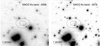 |
Fig. 1. VLT/NaCo images of the field of 1E 1613 in RCW 103 in 2006 and 2016. The ellipses show the 68% and 99% position uncertainty of 1E 1613. The source detected in 2016 at Ks = 20.68 ± 0.12 that previously was not detected (Ks > 21.2) is marked with two ticks. The same source is labeled “8” in Fig. 2 of Tendulkar et al. (2017). |
We also investigated a possible short-term variability of the new candidate counterpart of 1E 1613. To this aim, we generated images with 1000 s exposure time as well as with 2500 s exposure time by combining 20 and 50 consecutive frames with 50 s integration time, respectively. For each image, we performed astrometric and photometric calibration as described above for the master image, with similar accuracy. This allowed us to produce light curves with ∼1000 s and ∼2500 s binning for ∼380 and ∼900 sources, respectively, including the new candidate counterpart as well as all of the seven candidate counterparts mentioned by De Luca et al. (2008). As in our previous analysis (De Luca et al. 2008), we found a larger rms variability for fainter sources, which implies that our photometric measurements are contaminated by random errors (see discussion in De Luca et al. 2008). The new candidate counterpart (Ks ∼ 20.7) displays an rms of ∼0.22 mag and of ∼0.23 mag on the 1000 s and on the 2500 s timescales, respectively. These results are broadly consistent with the apparent rms variability for sources in the Ks magnitude range 20.0–21.0, which is of ∼0.18 mag and of ∼0.13 mag on the 1000 s (55 sources) and on the 2500 s timescale (335 sources), respectively. Thus, we cannot draw firm conclusions about a possible modulation of the flux of the new candidate counterpart. The same is true for all of the seven candidate counterparts mentioned by De Luca et al. (2008).
3. XMM-Newton observations and results
Two XMM-Newton observations of 1E 1613 were taken after the 2016 outburst, one on 2016 August 19–20 (Obs. ID 0743750201) and one on 2018 February 14 (Obs. ID 0805050101). The 2016 exposure lasted about 82.5 ks, and the EPIC pn (Strüder et al. 2001) was operated in Small Window mode (time resolution: 5.7 ms) and the MOS detectors (Turner et al. 2001) in Large Window mode (time resolution: 0.9 s); all cameras mounted the thin optical-blocking filter. The exposures of the MOS cameras were interrupted after ∼0.5 ks and later resumed, with a gap of ∼3.2 ks both in the MOS1 and MOS2 data. The 2018 pointing was 63 ks long and all the detectors were in Full Frame mode (time resolution: 73.4 ms for the pn and 2.7 s for the MOSs), using the thin filter for the pn and the medium filter for the MOSs. The second observation was affected by intervals of flaring particle background, which were removed using intensity filters on the light curves; this screening reduced by ∼20% the net exposure time in the pn and by a lesser amount in the MOS cameras (see Table 1 for more details).
XMM-Newton observations. In the second observation, the net exposure times are after the screening for proton flares.
The raw observation data files were processed with the Science Analysis Software (SAS; Gabriel et al. 2004) v.17.1. To extract the event lists and spectra, we used the same regions as were selected in De Luca et al. (2006): a circle with a radius of 15 arcsec centered on 1E 1613 and a circle with a radius of 20 arcsec with a center at  , Dec = −51 ° 02′38″ (J2000), a region where the surface brightness of the RCW 103 SNR is comparable to that of the surroundings of the source, to estimate the background. Spectra were rebinned so as to have a minimum of 30 counts per energy bin, and for each spectrum, the response matrix and ancillary files were generated with the SAS tasks rmfgen and arfgen. To convert the event times into the solar system barycenter, we used the task barycen.
The evolution of the flux, the spectral shape, and the pulse profile of 1E 1613 in the aftermath of the outburst have been studied in detail by Borghese et al. (2018) and Coti Zelati et al. (2018) over a period encompassing the two XMM-Newton observations. Here, we concentrate on the individual data sets.
The 6.67 h flux modulation is evident in both observations and apparently evolves from the complicate shape that is characteristic of the outbursts toward the nearly sinusoidal profile observed in quiescence (Fig. 2; see also Fig. 2 of De Luca et al. 2006 and Fig. 4 of Esposito et al. 2011). In the first observation, the high flux combined with the long exposure resulted in spectra with hundreds of thousands of source counts (> 2 × 10⁵ in the pn and > 105 in each MOS). In spectra of such high statistical quality, systematic (calibration) errors are important in the error budget, as can be seen by inspecting the fit residuals at the energies of the effective area edges, where large variations occur rapidly. For this reason we added to the spectra an energy-independent systematic uncertainty of 3% (see, e.g., Molendi & Gastaldello 2009).
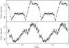 |
Fig. 2. Folded light curves of 1E 1613. Top panel: 2016 data set (A) and bottom panel: 2018 data set (B). The energy range is 1–10 keV, and both data sets were folded with epoch MJD 57619 in the FTOOLS task efold and the period of Esposito et al. (2011, P = 24 030.42 s). The profile apparently evolves from the complex multi-peak structure observed in high flux states to the simpler (nearly sinusoidal) shape observed in quiescence (see Fig. 2 of De Luca et al. 2006, Fig. 3 of Rea et al. 2016, and Fig. 4 of Esposito et al. 2011 for a collection of the pulse profiles that were observed in quiescence). |
The spectra may be modeled by a double blackbody or a blackbody-plus-power-law model and an absorption component. For the latter, we adopted the abundances by Wilms et al. (2000) and the Tübingen-Boulder interstellar medium (ISM) absorption model. The parameters derived from the spectral fits are similar to those from previous analyses (De Luca et al. 2006; Rea et al. 2016; Borghese et al. 2018) and are summarized in Table 2.
Summary of the spectral results.
Figure 3 shows the long-term evolution of the observed flux (the XMM-Newton data refer to the double-blackbody model).
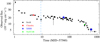 |
Fig. 3. Long-term light curve of 1E 1613 starting from the 2016 burst. The flux (not corrected for the absorption) is in the 0.5–10 keV band. Except for the XMM-Newton points, the data are from the Magnetar Outburst Online Catalog (MOOC, http://magnetars.ice.csic.es/; Coti Zelati et al. 2018) and the flux values were obtained from a double-blackbody fit. For some data points, the error bar is smaller than the symbol. The dashed line indicates the epoch of the VLT observation. |
Inspecting the light curves, we realized that they contained unusual features in the first observation. At least two long-lasting flares occurred, the first ∼32 ks after the start of the observation, the second at about 78 ks (see Fig. 4). They can be identified because (> 5 keV) they appear like spikes in the hard band. The first flare lasted approximately 1.2 ks and had a faster rise than decline; the second flare had a slightly more symmetric profile and lasted ∼2.2 ks. No similar events were found in the second observation.
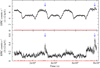 |
Fig. 4. Light curves of 1E 1613 from the 2016 observation (A) in the 1–12 keV range (top) and in a hard band (5–12 keV) (bottom). The time bin is 250 s. The background contribution is negligible and was not subtracted, but the background level in the proper energy band is shown in red in each panel. The arrows indicate the faint flares (more prominent in the hard band) that are discussed in Sect. 3. |
Extracting the spectra from the time intervals of the flares, we found that the spectral shapes of the two flares are very similar. As a first guess, we assumed that the flare emission is superimposed on the persistent emission, and we fit the flare spectra with a model consisting of the average spectrum of observation A plus an additional component, either a power law or a blackbody. The fits are essentially equally good; the additional component resembles the hard component of the average spectrum. In the blackbody fit, the temperature converges to a value that is compatible with the value of the hot blackbody in Table 2. In other words, the spectra of the flares are extremely similar to the spectrum of the persistent emission with an stronger hot component. This can be visually assessed in Fig. 5, where we show a simultaneous fit of the spectra of the average emission and of the two flares where all parameters are tied except for the hot blackbody normalization. The resulting radii are  and
and  km for the first and second flare, respectively (
 for 2756 degrees of freedom, d.o.f.). The corresponding luminosities are (5.7 ± 0.1) × 1034 and (6.1 ± 0.1) × 1034 erg s−1 (0.5–10 keV), that is, only ≈20–30% more than the average luminosity (but we note that both events occur at the maximum of the pulse profile, although not exactly at the same phase: they are separated by ∼1.9 cycles).
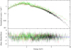 |
Fig. 5. Spectra of the flares (the data of the first are plotted in red, those of the second in green) compared with that of the average emission (in black). The model fit to the data is the double blackbody. For clarity, we plot only the pn points. Bottom: post-fit residuals. |
4. Discussion
In 2016, after hibernating for more than a decade, 1E 1613 entered a new phase of magnetar-like activity and produced the first outburst from this source that was monitored intensely and was also followed in hard X-rays and at IR wavelengths (Rea et al. 2016; D’Aì et al. 2016; Tendulkar et al. 2017; Borghese et al. 2018). All studies spotted strong similarities between this unusual source and magnetars, which underlines the possibility that the compact object might be a magnetar (De Luca et al. 2006). The space for a binary system was already narrow in view of the limit on the IR emission that was previously obtained by De Luca et al. (2008), but the ignition of 1E 1613 in the IR that was observed with HST by Tendulkar et al. (2017) strongly argues against the possibility of accretion onto the neutron star. The HST detection implies a brightening > 1.3 mag in the F160W filter band (H band, λ = 1.545 μm; Δλ = 0.29 μm FWHM) and > 1.8 mag in the F110W filter band (wide J, λ = 1.15 μm; Δλ = 0.5 μm FWHM). Our (non-simultaneous) VLT observation implies an increase in flux density of at least ∼0.5 mag in the Ks band. The extinction toward 1E 1613 is uncertain. The dust reddening mapped in its direction is AV = 36 (Schlafly & Finkbeiner 2011), and high extinction is indicated also by the colors of field stars (De Luca et al. 2008). On the other hand, much lower values are obtained from optical and IR observations of the SNR and from the NH measured in the X-ray observations (Oliva et al. 1989; Tendulkar et al. 2017). Following Tendulkar et al. (2017), we assume an AV from 3.6 to 36 but, as they note, a low AV seems more likely because it is suggested by measurements of 1E 1613 and its SNR, while the high values come from analyses of a vast field and unrelated stars. The IR-to-X-ray spectral energy distribution of 1E 1613 for the extreme values of AV is shown in Fig. 6 (which, we stress, must be taken with caution because the source is variable and the exposures are not simultaneous).
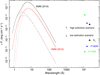 |
Fig. 6. Spectral energy distribution for 1E 1613 from X-rays to near IR. The XMM-Newton spectral models (double blackbody) are plotted in black for the 2016 data and in red for the 2018 data; the two blackbody components are plotted with the same colors and dashed lines. The black triangles indicate the June 2016 VLT values in the case of low and high extinction (AV from 3.6 to 36). The HST points are from Tendulkar et al. (2017) and the exposures were taken in August 2016 (similar values were found earlier, in July 2016). |
Propeller interaction with a surrounding fallback disk is often proposed as a possible explanation of the slow rotation of 1E 1613 (De Luca et al. 2006; Li 2007; Tong et al. 2016; Ho & Andersson 2017). Given the lack of constraints on the presence of pulsations in the VLT data, it is hard to tell whether the IR emission is of magnetospheric origin or is due to a disk heated by the enhanced emission of 1E 1613 during the outburst. In the case of low extinction, the Ks-to-X-ray flux ratio is ∼1.8 × 10⁻⁵, which is similar to the corresponding HST ratios and is in the range observed for magnetars and isolated neutron stars (Mignani 2011; Olausen & Kaspi 2014). With this assumption, the detection in itself therefore does not support the presence of a fallback disk around the star.
A careful analysis of the source light curves in X-rays revealed the presence of two flares with properties much at variance with those of canonical magnetar bursts. They last much longer (∼1 ks vs. 0.1–1 s), are less energetic (L ≈ 1034 erg s−1, exceeding the persistent luminosity by only ∼20%, vs. L ≳ 1038 erg s−1), and are softer, with a spectrum quite close to the hotter thermal component of the persistent flux. Because of their long duration, however, their fluence is rather high, ≈7 × 10⁻⁹ and 2 × 10⁻⁸ erg cm−2 for the first and second event, respectively, and comparable with standard short burst from magnetars (e.g., Aptekar et al. 2001; Götz et al. 2006; Göǧüş et al. 2000).
To the best of our knowledge, an event like this has not been observed before in a magnetar or in other classes of X-ray emitting isolated NSs. However, flares similar to those reported here might well have occurred in other sources and passed unnoticed. The strong similarity of the flare spectrum with the hotter thermal component seen in the persistent emission suggests a common origin. In magnetars, the latter is believed to come from a limited region on the star surface that is heated by dissipative processes. If the flares observed in 1E 1613 do come from the same hot spot, they would be hardly visible in a source with a period (≈0.1–10 s) much shorter than the flare duration (≈1 ks), as is the case of all the known X-ray pulsars. In this sense, 1E 1613 is unique because of its period, which is much longer than the flare duration. Further pursuing the idea that the flares originate from a spot on the star surface, they could be produced by some irregularities in the process responsible for the heating. Although the nature of such processes in magnetars is still debated (see, e.g., Turolla et al. 2015; Kaspi & Beloborodov 2017; Gourgouliatos & Esposito 2018, for recent reviews), we mention that if the star surface is heated by backflowing currents, an increase in luminosity by ∼20% can easily be explained by a change of the same order in the twist angle or in the potential drop that accelerates the charges (Beloborodov 2009). We also note that the second flare occurred approximately at the same rotational phase as the first, after ∼1.9 cycles. Although with just two events a coincidence cannot be excluded, this might indicate that they came from the same hot spot.
See the NaCo News Page at http://www.eso.org/sci/facilities/paranal/instruments/naco/news.html
Acknowledgments
The scientific results reported in this article are based on observations obtained with XMM-Newton, an ESA science mission with instruments and contributions directly funded by ESA Member States and NASA. Based on observations collected at the European Organisation for Astronomical Research in the Southern Hemisphere under ESO programmes 077.D-0764(A) and 297.D-5042(A). PE and ADL acknowledge funding in the framework of the project ULTraS (ASI–INAF contract N. 2017-14-H.0). FCZ is supported by a Juan de la Cierva fellowship.
References
- Aptekar, R. L., Frederiks, D. D., Golenetskii, S. V., et al. 2001, ApJ, 137, 227 [Google Scholar]
- Beloborodov, A. M. 2009, ApJ, 703, 1044 [NASA ADS] [CrossRef] [Google Scholar]
- Bertin, E., & Arnouts, S. 1996, A&AS, 117, 393 [NASA ADS] [CrossRef] [EDP Sciences] [Google Scholar]
- Bhadkamkar, H., & Ghosh, P. 2009, A&A, 506, 1297 [NASA ADS] [CrossRef] [EDP Sciences] [Google Scholar]
- Borghese, A., Coti Zelati, F., Esposito, P., et al. 2018, MNRAS, 478, 741 [NASA ADS] [CrossRef] [Google Scholar]
- Caswell, J. L., Murray, J. D., Roger, R. S., Cole, D. J., & Cooke, D. J. 1975, A&A, 45, 239 [NASA ADS] [Google Scholar]
- Coti Zelati, F., Rea, N., Pons, J. A., Campana, S., & Esposito, P. 2018, MNRAS, 474, 961 [NASA ADS] [CrossRef] [Google Scholar]
- D’Aì, A., Evans, P. A., Burrows, D. N., et al. 2016, MNRAS, 463, 2394 [NASA ADS] [CrossRef] [Google Scholar]
- De Luca, A. 2008, in 40 Years of Pulsars: Millisecond Pulsars, Magnetars and More, eds. C. Bassa, Z. Wang, A. Cumming, & V. M. Kaspi, AIP Conf. Proc., 983, 311 [NASA ADS] [CrossRef] [Google Scholar]
- De Luca, A. 2017, in International Conference Physics of Neutron Stars - 2017. 50 years after, St. Petersburg, Russian Federation, eds. G. G. Pavlov, J. A. Pons, P. S. Shternin, & D. G. Yakovlev, J. Phys. Conf. Ser., 932, 012006 [Google Scholar]
- De Luca, A., Caraveo, P. A., Mereghetti, S., Tiengo, A., & Bignami, G. F. 2006, Science, 313, 814 [NASA ADS] [CrossRef] [PubMed] [Google Scholar]
- De Luca, A., Mignani, R. P., Zaggia, S., et al. 2008, ApJ, 682, 1185 [NASA ADS] [CrossRef] [Google Scholar]
- Devillard, N. 1997, The Messenger, 87, 19 [NASA ADS] [Google Scholar]
- Esposito, P., Turolla, R., De Luca, A., et al. 2011, MNRAS, 418, 170 [NASA ADS] [CrossRef] [Google Scholar]
- Esposito, P., Rea, N., & Israel, G. L. 2018, in Timing Neutron Stars: Pulsations, Oscillations and Explosions, eds. T. Belloni, M. Mendez, & C. Zhang (Berlin: Springer), ASSL, in press [arXiv:1803.05716] [Google Scholar]
- Gabriel, C., Denby, M., Fyfe, D. J., et al. 2004, in Astronomical Data Analysis Software and Systems (ADASS) XIII, eds. F. Ochsenbein, M. G. Allen, & D. Egret (San Francisco, CA: ASP), ASP Conf. Ser., 314, 759 [Google Scholar]
- Götz, D., Mereghetti, S., Molkov, S., et al. 2006, A&A, 445, 313 [NASA ADS] [CrossRef] [EDP Sciences] [Google Scholar]
- Gourgouliatos, K. N., & Esposito, P. 2018, in The Physics and Astrophysics of Neutron Stars, eds. L. Rezzolla, P. M. Pizzochero, D. I. Jones, N. Rea, & I. Vidaña (Basel: Springer Nature Switzerland), 457, 57 [NASA ADS] [CrossRef] [Google Scholar]
- Göǧüş, E., Woods, P. M., Kouveliotou, C., et al. 2000, ApJ, 532, L121 [NASA ADS] [CrossRef] [Google Scholar]
- Ho, W. C. G., & Andersson, N. 2017, MNRAS, 464, L65 [NASA ADS] [CrossRef] [Google Scholar]
- Kaspi, V. M., & Beloborodov, A. M. 2017, ARA&A, 55, 261 [NASA ADS] [CrossRef] [Google Scholar]
- Lenzen, R., Hartung, M., Brandner, W., et al. 2003, in Instrument Design and Performance for Optical/Infrared Ground-based Telescopes, eds. M. Iye, & A. F. M. Moorwood (Bellingham: SPIE), SPIE Conf. Ser., 4841, 944 [Google Scholar]
- Li, X. 2007, ApJ, 666, L81 [NASA ADS] [CrossRef] [Google Scholar]
- Liu, X. W., Xu, R. X., van den Heuvel, E. P. J., et al. 2015, ApJ, 799, 233 [NASA ADS] [CrossRef] [Google Scholar]
- Mignani, R. P. 2011, AdSpR, 47, 1281 [NASA ADS] [CrossRef] [Google Scholar]
- Molendi, S., & Gastaldello, F. 2009, A&A, 493, 13 [NASA ADS] [CrossRef] [EDP Sciences] [Google Scholar]
- Olausen, S. A., & Kaspi, V. M. 2014, ApJ, 212, 6 [Google Scholar]
- Oliva, E., Moorwood, A. F. M., & Danziger, I. J. 1989, A&A, 214, 307 [NASA ADS] [Google Scholar]
- Pizzolato, F., Colpi, M., De Luca, A., Mereghetti, S., & Tiengo, A. 2008, ApJ, 681, 530 [NASA ADS] [CrossRef] [Google Scholar]
- Popov, S. B., Kaurov, A. A., & Kaminker, A. D. 2015, PASA, 32, e018 [NASA ADS] [CrossRef] [Google Scholar]
- Rea, N., Borghese, A., Esposito, P., et al. 2016, ApJ, 828, L13 [NASA ADS] [CrossRef] [Google Scholar]
- Rousset, G., Lacombe, F., Puget, P., et al. 2003, in Adaptive Optical System Technologies II, eds. P. L. Wizinowich, & D. Bonaccini, (Bellingham: SPIE), SPIE Conf. Ser., 4839, 140 [Google Scholar]
- Schlafly, E. F., & Finkbeiner, D. P. 2011, ApJ, 737, 103 [NASA ADS] [CrossRef] [Google Scholar]
- Strüder, L., Briel, U., Dennerl, K., et al. 2001, A&A, 365, L18 [NASA ADS] [CrossRef] [EDP Sciences] [Google Scholar]
- Tendulkar, S. P., Kaspi, V. M., Archibald, R. F., & Scholz, P. 2017, ApJ, 841, 11 [NASA ADS] [CrossRef] [Google Scholar]
- Tong, H., Wang, W., Liu, X. W., & Xu, R. X. 2016, ApJ, 833, 265 [NASA ADS] [CrossRef] [Google Scholar]
- Tuohy, I., & Garmire, G. 1980, ApJ, 239, L107 [NASA ADS] [CrossRef] [Google Scholar]
- Turner, M. J. L., Abbey, A., Arnaud, M., et al. 2001, A&A, 365, L27 [NASA ADS] [CrossRef] [EDP Sciences] [Google Scholar]
- Turolla, R., Zane,, S., & Watts, A. L. 2015, Rep. Progr. Phys., 78, 116901 [Google Scholar]
- Wilms, J., Allen, A., & McCray, R. 2000, ApJ, 542, 914 [NASA ADS] [CrossRef] [Google Scholar]
All Tables
XMM-Newton observations. In the second observation, the net exposure times are after the screening for proton flares.
All Figures
|
Fig. 1. VLT/NaCo images of the field of 1E 1613 in RCW 103 in 2006 and 2016. The ellipses show the 68% and 99% position uncertainty of 1E 1613. The source detected in 2016 at Ks = 20.68 ± 0.12 that previously was not detected (Ks > 21.2) is marked with two ticks. The same source is labeled “8” in Fig. 2 of Tendulkar et al. (2017). |
| In the text | |
|
Fig. 2. Folded light curves of 1E 1613. Top panel: 2016 data set (A) and bottom panel: 2018 data set (B). The energy range is 1–10 keV, and both data sets were folded with epoch MJD 57619 in the FTOOLS task efold and the period of Esposito et al. (2011, P = 24 030.42 s). The profile apparently evolves from the complex multi-peak structure observed in high flux states to the simpler (nearly sinusoidal) shape observed in quiescence (see Fig. 2 of De Luca et al. 2006, Fig. 3 of Rea et al. 2016, and Fig. 4 of Esposito et al. 2011 for a collection of the pulse profiles that were observed in quiescence). |
| In the text | |
|
Fig. 3. Long-term light curve of 1E 1613 starting from the 2016 burst. The flux (not corrected for the absorption) is in the 0.5–10 keV band. Except for the XMM-Newton points, the data are from the Magnetar Outburst Online Catalog (MOOC, http://magnetars.ice.csic.es/; Coti Zelati et al. 2018) and the flux values were obtained from a double-blackbody fit. For some data points, the error bar is smaller than the symbol. The dashed line indicates the epoch of the VLT observation. |
| In the text | |
|
Fig. 4. Light curves of 1E 1613 from the 2016 observation (A) in the 1–12 keV range (top) and in a hard band (5–12 keV) (bottom). The time bin is 250 s. The background contribution is negligible and was not subtracted, but the background level in the proper energy band is shown in red in each panel. The arrows indicate the faint flares (more prominent in the hard band) that are discussed in Sect. 3. |
| In the text | |
|
Fig. 5. Spectra of the flares (the data of the first are plotted in red, those of the second in green) compared with that of the average emission (in black). The model fit to the data is the double blackbody. For clarity, we plot only the pn points. Bottom: post-fit residuals. |
| In the text | |
|
Fig. 6. Spectral energy distribution for 1E 1613 from X-rays to near IR. The XMM-Newton spectral models (double blackbody) are plotted in black for the 2016 data and in red for the 2018 data; the two blackbody components are plotted with the same colors and dashed lines. The black triangles indicate the June 2016 VLT values in the case of low and high extinction (AV from 3.6 to 36). The HST points are from Tendulkar et al. (2017) and the exposures were taken in August 2016 (similar values were found earlier, in July 2016). |
| In the text | |
Current usage metrics show cumulative count of Article Views (full-text article views including HTML views, PDF and ePub downloads, according to the available data) and Abstracts Views on Vision4Press platform.
Data correspond to usage on the plateform after 2015. The current usage metrics is available 48-96 hours after online publication and is updated daily on week days.
Initial download of the metrics may take a while.