| Issue |
A&A
Volume 625, May 2019
|
|
|---|---|---|
| Article Number | A2 | |
| Number of page(s) | 25 | |
| Section | Catalogs and data | |
| DOI | https://doi.org/10.1051/0004-6361/201834918 | |
| Published online | 30 April 2019 | |
The fourth data release of the Kilo-Degree Survey: ugri imaging and nine-band optical-IR photometry over 1000 square degrees
1
Leiden Observatory, Leiden University, Box 9513, 2300 RA Leiden, The Netherlands
e-mail: This email address is being protected from spambots. You need JavaScript enabled to view it.
2
Scottish Universities Physics Alliance, Institute for Astronomy, University of Edinburgh, Royal Observatory, Blackford Hill, Edinburgh EH9 3HJ, UK
3
Astronomisches Institut, Ruhr-Universität Bochum, Universitätsstrasse 150, 44801 Bochum, Germany
4
Argelander-Institut für Astronomie, Auf dem Hügel 71, 53121 Bonn, Germany
5
Kapteyn Astronomical Institute, University of Groningen, PO Box 800 9700 AV Groningen, The Netherlands
6
Center for Theoretical Physics, Polish Academy of Sciences, al. Lotników 32/46, 02-668 Warsaw, Poland
7
Shanghai Astronomical Observatory, Nandan Road 80, Shanghai 200030, PR China
8
INAF – Osservatorio Astronomico di Capodimonte, Via Moiariello 16, 80131 Napoli, Italy
9
Department of Physics, University of Oxford, Denys Wilkinson Building, Keble Road, Oxford OX1 3RH, UK
10
School of Physics and Astronomy, Sun Yat-sen University, Guangzhou, 519082 Zhuhai Campus, PR China
11
Dept.of Physics “Ettore Pancini”, Università Federico II, 80126 Napoli, Italy
12
INAF – Osservatorio Astronomico di Padova, Via dell’Osservatorio 5, 35122 Padova, Italy
13
School of Physics and Astronomy, Queen Mary University of London, Mile End Road, London E1 4NS, UK
14
INAF – Osservatorio Astrofisico di Arcetri, Largo Enrico Fermi 5, 50125 Firenze, Italy
Received:
18
December
2018
Accepted:
14
March
2019
Abstract
Context. The Kilo-Degree Survey (KiDS) is an ongoing optical wide-field imaging survey with the OmegaCAM camera at the VLT Survey Telescope, specifically designed for measuring weak gravitational lensing by galaxies and large-scale structure. When completed it will consist of 1350 square degrees imaged in four filters (ugri).
Aims. Here we present the fourth public data release which more than doubles the area of sky covered by data release 3. We also include aperture-matched ZYJHKs photometry from our partner VIKING survey on the VISTA telescope in the photometry catalogue. We illustrate the data quality and describe the catalogue content.
Methods. Two dedicated pipelines are used for the production of the optical data. The ASTRO-WISE information system is used for the production of co-added images in the four survey bands, while a separate reduction of the r-band images using the THELI pipeline is used to provide a source catalogue suitable for the core weak lensing science case. All data have been re-reduced for this data release using the latest versions of the pipelines. The VIKING photometry is obtained as forced photometry on the THELI sources, using a re-reduction of the VIKING data that starts from the VISTA pawprints. Modifications to the pipelines with respect to earlier releases are described in detail. The photometry is calibrated to the Gaia DR2 G band using stellar locus regression.
Results. In this data release a total of 1006 square-degree survey tiles with stacked ugri images are made available, accompanied by weight maps, masks, and single-band source lists. We also provide a multi-band catalogue based on r-band detections, including homogenized photometry and photometric redshifts, for the whole dataset. Mean limiting magnitudes (5σ in a 2″ aperture) and the tile-to-tile rms scatter are 24.23 ± 0.12, 25.12 ± 0.14, 25.02 ± 0.13, 23.68 ± 0.27 in ugri, respectively, and the mean r-band seeing is 0.″70.
Key words: galaxies: general / surveys / large-scale structure of Universe
© ESO 2019
1. Introduction: the Kilo-Degree and VIKING surveys
High-fidelity images of the sky are one of the most fundamental kinds of data for astronomy research. While for many decades photographic plates dominated optical sky surveys, the advent of large-format CCD detectors for astronomy opened up the era of digital, high resolution, high sensitivity, linear-response images.
The ESO VLT Survey Telescope (VST; Capaccioli & Schipani 2011; Capaccioli et al. 2012) at ESO’s Paranal observatory was specifically designed for wide-field, optical imaging. Its focal plane contains the square 268-million pixel CCD mosaic camera OmegaCAM (Kuijken 2011) that covers a  area at
  pitch, and the site and telescope optics (with actively controlled primary and secondary mirrors) ensure an image quality that is sub-arcsecond most of the time, and that does not degrade towards the corners of the field. Since starting operations in October 2011, more than half of the available time on the telescope has been used for a set of three wide-area “Public Imaging Surveys” for the ESO community. The Kilo-Degree Survey (KiDS; de Jong et al. 2013)1 is the deepest of these, and the one that exploits the best observing conditions.
KiDS was designed as a cosmology survey, to study the galaxy population out to redshift ∼1 and in particular to measure the effect on galaxy shapes due to weak gravitational lensing by structure along the line of sight. By combining galaxy shapes with photometric redshift estimates it is possible to locate the redshift at which the gravitational lensing signal originates, and hence to map out the growth of large-scale structure, an important aspect of the evolution of the Universe and a key cosmology probe. Together with KiDS, two other major surveys are engaged in such measurements: the Dark Energy Survey (DES; Dark Energy Survey Collaboration 2005)2 and the HyperSuprimeCam survey (HSC; Aihara et al. 2018)3, and all three have reported intermediate cosmology results (Hildebrandt et al. 2017, henceforth KiDS450; Troxel et al. 2018; Hikage et al. 2019). Their precision is already such that the measurements can constrain some parameters in the cosmological model to a level that is comparable to what is achieved from the cosmic microwave background anisotropies (Planck Collaboration VI 2018). Since ground-based surveys are limited fundamentally by the atmospheric disturbance on galaxy shapes and photometry, space missions Euclid (Laureijs et al. 2011) and later WFIRST (Spergel et al. 2015) are planned to increase the fidelity of such studies further.
To meet its primary science goal KiDS observes the sky in four bands: u, g, r and i. The r band is used in dark time during the best seeing conditions ( ), to make deep images for the measurement of galaxy shapes. In order to provide colours for photometric redshift estimates of the same sources, the r-band data are supplemented with g- and u-band data taken in dark time of progressively worse seeing conditions (
 and
and  , respectively), and with i-band data taken in grey or bright moon time with a mild seeing constraint (
 ). All observations consist of multiple dithered exposures to minimize the effect of gaps between the CCD’s in the mosaic. Observing constraints and exposure times are summarized in Table 1.
KiDS observing strategy: observing condition constraints and exposure times.
KiDS is targeting around 1350 square degrees of extragalactic sky, in two patches to ensure year-round observability. The Northern patch, KiDS-N, contains two additional smaller areas: KiDS-N-W2, which coincides with the G9 patch of the GAMA survey (Driver et al. 2011), and KiDS-N-D2, a single pointing on the COSMOS field. In a coordinated effort over the same part of the sky, the VISTA Kilo-degree INfrared Galaxy survey (VIKING; Edge et al. 2013) on the nearby VISTA telescope added the five bands Z, Y, J, H and Ks. VIKING observations are complete4 and available in the ESO archive5. Table 2 and Fig. 1 show the full KiDS footprint on the sky, as well as the part that is covered by the data contained in this data release (KiDS-ESO-DR4, or DR4 for short). The fields that were previously released under DR1+2+3 are also indicated: this is the area that was used for the KiDS450 cosmic shear analysis, with the corresponding shape/photometric redshift catalogue released as DR3.1.
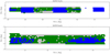 |
Fig. 1. Sky distribution of survey tiles released in KiDS-ESO-DR4. Tiles shown in green are released for the first time; those in blue were included in the earlier data releases (DR1+2+3) but have been reprocessed for DR4. The full KiDS+VIKING area (∼1350deg2) is shown in grey. Top: KiDS-North. Bottom: KiDS-South. The single pointing at RA = 150deg is centred on the COSMOS/CFHTLS D2 field. |
In order to improve the fidelity of the photometric redshift-based tomography, and to enable inclusion of high-value sources in the redshift range 0.9–1.2, Hildebrandt et al. (2018) added VIKING photometry to the KiDS-450 data set, as described in Wright et al. (2018). The resulting cosmological parameter constraints of this new analysis, dubbed “KV450”, are fully consistent with KiDS450. DR4 incorporates the methodology developed for KV450 and includes VIKING photometry for all sources. Of all wide-area surveys, this makes it the one with by far the deepest near-IR data.
Though designed for the primary cosmology science case (KiDS450; Joudaki et al. 2017; van Uitert et al. 2018; Köhlinger et al. 2017; Harnois-Déraps et al. 2017; Amon et al. 2018; Shan et al. 2018; Martinet et al. 2018; Giblin et al. 2018; Asgari et al. 2019), KiDS data are also being used for a variety of other studies, including the galaxy-halo connection (van Uitert et al. 2016, 2017), searches for strongly lensed galaxies (Petrillo et al. 2019) and quasars (Spiniello et al. 2018; Sergeyev et al. 2018), solar system objects (Mahlke et al. 2018), photometric redshift machine learning method development (Amaro et al. 2019; Bilicki et al. 2018), studies of galaxy evolution (Tortora et al. 2018a,b; Roy et al. 2018), bias (Dvornik et al. 2018), environment (Brouwer et al. 2016, 2018; Costa-Duarte et al. 2018) and morphology (Kelvin et al. 2018), galaxy group properties (Viola et al. 2015; Jakobs et al. 2018), galaxy cluster searches (Maturi et al. 2019; Bellagamba et al. 2019), intrinsic alignment of galaxies (Georgiou et al. 2019; Johnston et al. 2019), satellite halo masses (Sifón et al. 2015), and searches for luminous red galaxies (Vakili et al. 2018) and quasars (Nakoneczny et al. 2019).
The outline of this paper is as follows. Section 2 is a discussion of the contents of KiDS-ESO-DR4. Section 3 summarises the differences in terms of processing and data products with respect to earlier releases. Sections 4 and 5 describe the single-band data products and the KiDS+VIKING nine-band catalogue, respectively. Section 6 illustrates the data quality. Data access routes are summarised in Sect. 7 and a summary and outlook towards future data releases is provided in Sect. 8. The appendix gives a full listing of the information included in the images and catalogues, and of the data structure.
2. The fourth KiDS data release
Unlike the previous incremental KiDS data releases, KiDS-ESO-DR4 represents a complete re-reduction of all the data using improved pipeline recipes and procedures. The differences will be described below. In terms of content of the data release, the main changes with respect to the earlier releases (de Jong et al. 2015, 2017) are the more than doubling of the area, and the inclusion of photometry from the near-IR VIKING images into the multi-band catalogue. Whereas the sky coverage of the earlier data releases was still quite fragmented, DR4’s greater homogeneity will for the first time enable wide-area studies over the full length of the survey patches.
KiDS observations consist of individual square-degree tiles. Each tile is covered by a set of five (four in u) dithered exposures with OmegaCAM/VST, consisting of 32 individual CCD images each. The dither step sizes are matched to the gaps between CCD’s (25″ in RA, 85″ in declination), to ensure that each part of the tile is covered by at least three (two in u) sub-exposures. Overlaps between adjacent tiles are small, of order 5%. All observations in a single band are taken in immediate succession (KiDS is not designed for variability measurements), but there is no constraint on the time between observations of any given tile in the different filters. Typically the shutter is closed for 35–60 s between the sub-exposures to allow for CCD readout, telescope repointing and active optics adjustments.
With little exception, the DR4 data comprise all KiDS tiles for which the 4-band observations had been taken by January 24th, 2018. Over half of the data is from after mid-2015, which is when the VST saw several improvements that affect the quality of the data (and improved operational efficiency as well, see Fig. 2). The two main improvements were (i) the baffling of the telescope was improved to the point that stray light from sources outside the field of view of the camera was drastically reduced; and (ii) the on-line image analysis system (based on simultaneous pre- and post-focus star images at the edge of the field of view) was modified to control also the tilt of the secondary mirror, improving pointing and especially off-axis image quality.
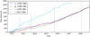 |
Fig. 2. Progress of the KiDS observations at the VST, in the four survey bands. Each Observing Block (OB) produces a square-degree co-added image. The i-band data, for which data taking was significantly faster because of less competition for bright time on the telescope, had covered the originally planned 1500 square degree footprint by the time it was decided to limit the survey to the 1350 square degree area that comprise the completed VIKING area. The dashed lines indicate the cutoff dates for KiDS-ESO data releases 1–4. |
Figure 3 shows the distributions of key data quality parameters of the observations: point spread function (PSF) full width at half maximum (FWHM), average PSF ellipticity and limiting magnitude. It illustrates that the global quality of the DR4 data is very similar to the earlier KiDS data releases. Limiting AB magnitudes (5σ in 2″ aperture) are 24.23 ± 0.12, 25.12 ± 0.14, 25.02 ± 0.13, 23.68 ± 0.27 in ugri, respectively, with the error bars representing the RMS scatter from tile to tile. The mean seeing in r band is  .
.
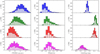 |
Fig. 3. Distributions of tile-by-tile data quality parameters for the KiDS DR4 data, grouped by filter, from top to bottom u, g, r and i. The light-coloured histograms represent the subset of the data that was previously released in DR1+2+3. Left: seeing. The differences between the bands reflect the observing strategy of reserving the best-seeing dark time for r-band observations. Middle column: average PSF ellipticity ⟨|epsf|⟩, where e is defined as 1 − b/a for major/minor axis lengths a and b. Right: limiting AB magnitude (5σ in a 2″ aperture). The wider distribution of the i-band observations is a caused by variations in the moon illumination, since the i-band data were mostly taken in bright time. |
The KiDS images were processed with two independent pipelines, as was the case for the KiDS-450 weak lensing analysis that was based on KiDS-ESO-DR3. The ASTRO-WISE pipeline and data reduction environment (McFarland et al. 2013)6 was used to produce stacked images in the four bands, from which the photometry in the catalogues is obtained. The THELI pipeline (Erben et al. 2005)7, which is optimised for weak lensing measurements, was used for a separate reduction of the r-band data only. In order to have consistent source lists, the detection and astrometry of the r-band sources is performed on these THELI images (which are also the ones which are used for the weak lensing measurements). This detection catalogue is then used as the basis of list-driven “forced” photometry on the u, g, r and i ASTRO-WISE stacked images and the VIKING Z, Y, J, H and Ks images8. The data flow is summarized in Fig. 4.
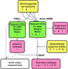 |
Fig. 4. Schematic representation of the DR4 processing steps and content. Yellow boxes show the input data from VST and VISTA, green indicates image products, and source lists are shown in pink. The lensfit-based lensing measurements – initially not released in DR4 – are shown as dotted lines. |
The set of KiDS-ESO-DR4 data products includes 5030 separate co-added images (1006 square-degree tiles in the ugri filters, plus the separate r-band co-adds from THELI), with corresponding weight and mask flag images. The images are photometrically and astrometrically calibrated using a combination of nightly photometric calibration information, the Gaia DR2 photometry (Brown et al. 2018) with stellar locus regression, and the SDSS and 2MASS astrometry (Alam et al. 2015; Skrutskie et al. 2006). Each image has a corresponding source catalogue as well. In addition, catalogues of nine-band ugriZYJHKs photometry are provided containing list-driven (i.e., forced), PSF- and aperture-matched photometry using the GAAP technique (Kuijken et al. 2015), applied to the KiDS tiles and the overlapping VIKING data.
3. Data processing
For details of the image processing pipelines we refer to the description in the DR1/2 and DR3 release papers (de Jong et al. 2015, henceforth DR1/2 and de Jong et al. 2017, henceforth DR3), noting the changes described in Sects. 3.1 and 3.2 below.
The DR4 catalogues are of two types: single-band catalogues for the four KiDS bands, and a combined nine-band catalogue that includes KiDS and VIKING photometry for the r-band detected sources.
3.1. Changes to the ASTRO-WISE image processing pipeline
3.1.1. Co-added image creation
The production of KiDS-ESO-DR4 includes 4 × 1006 OmegaCAM tiles, which required some 611 000 individual CCD exposures, as well as associated calibration observations, to be processed. The automatic processing steps followed closely those described in DR3. Individual CCD exposures are corrected for electronic crosstalk, bias corrected, flat-fielded, illumination corrected and (for i band only) fringe-subtracted. New coefficients were determined for the electronic crosstalk correction between CCD’s ESO_CCD_#95 and ESO_CCD_#96 (see DR1/2) with validity periods determined by maintenance or changes to the instrument; these are listed in Table 3. An automatic mask is also generated for each CCD, which marks the location of saturated, hot, and cold pixels, as well as satellite tracks identified through a Hough transform analysis.
Applied cross-talk coefficients.
These “reduced science frames” are then astrometrically calibrated and regridded using the SCAMP and SWARP software (Bertin et al. 2002; Bertin 2006, 2010a,b), in two steps: first a “local” step establishes a per-detector solution using the 2MASS stars in the frame9, and then these solutions are refined using SCAMP into a tile-wide “global solution” for the full co-added stacked image that uses the information from fainter overlapping objects. For DR4 the astrometric solution was made more robust by starting from a model of the focal plane that accounts for detector array lay-out and instrument optics distortion, and using this as input to SCAMP. Using SWARP, the global astrometric solution is then used to resample each CCD exposure into a “regridded science frame”, with a uniform  pixel grid with tangent projection centred on the nominal tile centre. During this step the background, determined by interpolating a 3 × 3 median-filtered map of background estimates in 128 × 128 pixel blocks, is subtracted. Finally these regridded images are co-added, taking account of the weight maps generated by SWARP, and the masks. Each co-added image is about 18 500 × 19 500 pixels in size, and takes up about 1.5 Gbyte of storage. For every co-added image a mask that flags reflection haloes of bright stars in the field is also produced, using the PULECENELLA code developed for DR1/2 (see Sect. 4).
12 × 12 binned versions of the co-added images (at two contrast settings) and of the weight image are then visually inspected, together with a set of diagnostic plots that show the PSF ellipticity and size as function of position on the field, astrometry solution residuals, and the PSF size before and after co-addition. The main issues that get flagged at this stage are (i) residual satellite tracks (ii) background features associated with stray light casting shadows of the baffles mounted above the CCD bond wires (iii) unstable CCDs (gain jumps) (iv) residual fringing in the background of the i-band images or (v) large-scale reflections. In DR3 any issues found at this stage were addressed by masking the co-added image, even though in many cases the problem only affected one sub-exposure. In DR4 issues (i)–(iii) were solved with new procedures, as described below. The other cases are still in the data: the residual fringes are not corrected for but will be fixed with re-observations of the full survey footprint in the i band, and large-scale reflections need to be masked manually or otherwise identified in the catalogues as groups of sources with unusual colours.
The new procedures for removing residual satellite tracks, bond wire baffle features, and unstable CCDs, involve a minimum of manual intervention. The satellite tracks are marked by clicking on their ends on a display of the inspection JPG images, after which an automatic procedure converts the pixel positions to sky coordinates, checks which of the sub-exposures that contribute to the co-added image contains the track, measures the track’s width, and updates the corresponding CCDs’ masks before stacking anew. Similarly, the bond wire baffle features have a typical width and all the inspector needs to do is to indicate whether the shadow is visible on the upper, lower or both sides of the baffles, so that the corresponding lines in the CCD images can be masked. Unstable CCDs are simply removed from the list of exposures to be co-added.
3.1.2. PSF Gaussianization and GAAP photometry
The Gaussian Aperture and PSF (GAAP) photometry method (Kuijken et al. 2015) developed for KiDS multi-band photometry was improved further. GAAP entails (i) convolving each image with a spatially variable kernel designed to render the PSF homogeneous and Gaussian, (ii) defining a pre-seeing Gaussian elliptical aperture function for every source, and (iii) for every band deconvolving this aperture by the corresponding Gaussianized PSF and performing aperture photometry. The method is superior to traditional techniques such as dual-image mode SEXTRACTOR measurements as it explicitly allows for PSF differences between exposures in multiple bands, and it reduces noise by measuring colours from the highest SNR part of the sources. A demonstration of the improvement provided by GAAP photometry is given in Hildebrandt et al. (2012). GAAP photometry gives colours that are corrected for PSF differences, but when the source is more extended than the aperture function the fluxes are underestimates of the total flux. For stars and other unresolved sources GAAP fluxes are total fluxes.
For DR4 we have modified the procedure for step (i). We still use the several thousand stars in each image as samples of the PSF, but rather than first modelling the PSF P as a spatially varying, truncated shapelet expansion, from which the convolution kernel is then constructed in shapelet coefficient space, we now directly solve for the kernel shapelet coefficients that give a Gaussian PSF in pixel space. Thus we obtain the kernel coefficients kabc of the shapelet components  as the least-squares solution of
={\exp \left[{-\left(x^2+y^2\right)/2\beta _{\rm g}^2}\right]\over 2\pi \beta _{\rm g}^2}\cdot \end{aligned} $$](/articles/aa/full_html/2019/05/aa34918-18/aa34918-18-eq22.gif) (2)
(2)
As in DR3, the size βg of the target Gaussian is set to 1.3 times the median dispersion of Gaussian fits to the stars in the image. The fit of Eq. (2) is performed over all pixels out to 15βg from the centre of each star. In our implementation we use terms with β1 = βg, a + b ≤ 8 plus a set of wider shapelets with β2 = 2.5βg, 3 ≤ a + b ≤ 6 specifically designed to model the wings of the kernel better. The large-β shapelets with a + b < 3 are not included in the series as they are not sufficiently orthogonal to the small-β terms.
3.1.3. Photometric calibration using Gaia and stellar locus regression
All KiDS “reduced science frame” images are initially put on a photometric scale by using nightly zeropoints derived from standard star observations taken in the middle of the night. For DR4, these zeropoints are refined with a combination of Stellar Locus Regression (SLR) and calibration to Gaia photometry. We use GAAP photometry for the stars: this is appropriate since for unresolved sources the GAAP magnitudes correspond to the total flux of the source.
With the advent of Gaia Data Release 2 (Brown et al. 2018) a deep, homogeneously calibrated, optical all-sky catalogue is now available. Each KiDS tile contains several thousand Gaia stars, with broad-band photometry measurements that are individually accurate to better than 0.01 mag10. KiDS DR4 photometry is calibrated to the Gaia DR2 catalogue in two steps. First, we calibrate the colours u − g, g − r and r − i by comparing the stellar colour-colour diagrams to fiducial sequences, using the “stellar locus regression” described in DR3. Based on the work of Ivezić et al. (2004), four principal colours P2s, P2w, P2x and P2k were initially used to derive colour offsets (see appendix B of KiDS450). After this procedure, while validating the results by comparing the magnitudes of stars in KiDS-N and SDSS, we found that the P2k principal colour, which is the most sensitive to the u band, gave unreliable results. The u-band zeropoints were therefore determined using a modified procedure, which was found to be more robust, as follows. For stars in Gaia with dereddened KiDS GAAP colour (g − r)0 between 0.15 and 0.8 and u < 21, the quantity
![Mathematical equation: $$ \begin{aligned} \mathcal{U}=g_0 + 2(g-r)_0 +0.346 + \max \left\{ 0, 2 \left[ 0.33-(g-r)_0\right]\right\} - f(b) \end{aligned} $$](/articles/aa/full_html/2019/05/aa34918-18/aa34918-18-eq23.gif) (3)
(3)
is a good predictor of the SDSS u magnitude. The Galactic latitude dependence f(b), shown in Fig. 5, can be fitted as
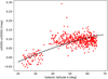 |
Fig. 5. Residual u-band magnitude variation when Eq. (3) is used without a dependence on Galactic latitude b (i.e., f(b)=0). Each point shows the average offset uKiDS − uSDSS for the calibration stars in a separate KiDS-N tile. The line represents the Galactic latitude correction of Eq. (4). |
 (4)
(4)
Stars closer to the Galactic plane are fainter in u than the mean (u − g, g − r) colour–colour relation predicts, as is expected if the high-latitude sample is dominated by halo stars of lower metallicity than the disk stars found at low b. Since KiDS-N spans latitudes from 22° to 66°, the correction is significant. KiDS-S covers latitudes from the South Galactic Pole to −53°, and though we cannot test the latitude dependence for this part of the survey because of a lack of a suitable calibration data set, we have applied the same correction. We therefore adjust the KiDS u-band zeropoints in each tile until the average 𝒰 − u = 0, with an iterative clipping of outliers more than 0.1 mag from the mean relation. For applications where u-band photometry is critical, we caution that because of the uncertain functional form of the latitude dependence, currently the calibration of this band is subject to a residual uncertainty of up to 0.05 mag.
The zeropoint of the r-band magnitude is then tied to Gaia by matching the dereddened (r − G, g − i) relation to the one followed by the stars in the SDSS–KiDS overlap region (Fig. 6). As reported in DR3, there is a slight colour term between the SDSS and KiDS r filters: we have arbitrarily forced the KiDS and SDSS r-band zeropoints to agree for stars of (g − i)0 = 0.8, adopting
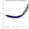 |
Fig. 6. Colour–colour relation used to calibrate the KiDS r-band measurements to the Gaia G-band catalogue, for an example tile. The blue points and the box indicate the dereddened (g − i) colour range for the stars used, and the ±0.05 mag iterative clipping width about the fiducial sequence. The shape of the sequence is determined from the overlap area between KiDS-N and SDSS. |
![Mathematical equation: $$ \begin{aligned} r_{\rm KiDS}-r_{\rm SDSS}=-0.02 [(g-i)_0-0.8]. \end{aligned} $$](/articles/aa/full_html/2019/05/aa34918-18/aa34918-18-eq25.gif) (5)
(5)
For DR4, extinction corrections were derived using the Schlegel et al. (1998)E(B − V) map in combination with the RV = 3.1 extinction coefficients from Schlafly & Finkbeiner (2011)11. For the ugri filters we adopt the corresponding SDSS filter values. Since the VISTA bands were not included in the Schlafly & Finkbeiner (2011) tables, as an approximation we have taken the values for SDSS z, LSST y, and UKIRT JHK filters. From a regression of rSDSS − G vs. E(B − V) we derive the G-band extinction coefficient as AG/Ar = 0.96. Given that E(B − V) values in the KiDS tiles are typically below 0.05 mag, residual uncertainties in these coefficients are of little consequence. The adopted extinction coefficients are summarised in Table 4.
Extinction coefficients Rf = Af/E(B − V) used in this work, from Schlafly & Finkbeiner (2011; SF11).
This direct, tile-by-tile calibration of the KiDS photometry to Gaia obviates the need for the overlap photometry that was used in DR3. Effectively, we are tying KiDS to the Gaia DR2 G-band photometry, and anchoring it to the SDSS calibration. Specifically, calibrating each KiDS tile to Gaia DR2 involves the following steps:
-
Select Gaia stars in the tile area with 16.5 < G < 20, and with unflagged photometric measurements.
-
Keep those stars with SLR-calibrated, dereddened (g − i)0 colours in the range [0.4, 1.8].
-
Predict dereddened (r − G)0 values from these (g − i)0 colours using the following relation, obtained by fitting the difference between the predicted rKiDS (from Eq. (5)) and the measured G in the KiDS-SDSS overlap region:
 (6)
(6)where y = (g − i)0 − 0.8 (see Fig. 6).
-
Determine the median offset between this fiducial r − G and the measured value, using iterative clipping.
-
Apply this median offset to the ugri magnitudes for all sources in the tile.
Figure 7 shows the distribution of tile-by-tile zeropoint corrections that have been applied to the magnitudes in the catalogues. Typical values are of the order of 0.05–0.1 mag, and about twice that in the u band.
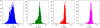 |
Fig. 7. Distribution of the u, g, r and i zeropoint corrections using the stellar locus regression plus Gaia calibration. |
Note that the SLR procedure aligns the dereddened stellar loci of all the tiles, assuming that all the dust is in the foreground and not mixed in with the stars (which is a reasonable assumption given the high Galactic latitude and bright-end limit of the calibration stars).
In DR4 all GAAP photometry is performed twice, with minimum aperture settings MIN_APER=  and
and  (see Sect. 5 below). The photometric zeropoint determinations are also performed with both settings, and the one based on the largest number of stars with valid measurements is recorded in the header of the images and single-band source catalogues with the DMAG keyword. CALMINAP gives the value of MIN_APER that was used for the calibration, and CALSTARS is the number of Gaia stars with valid measurements.
3.2. Changes to the THELI pipeline
In KiDS450, the THELI pipeline was used to process the r-band images for the weak lensing analysis, which resulted in two different r-band source catalogues with multi-band photometry (DR3 and the “lensing catalogue” DR3.1). For DR4 we unify the analysis, using the r-band sources detected on the THELI co-added images as the basis of the multi-band photometry as well as the forthcoming lensing analyses.
Compared to DR3, the main change for DR4 is the inclusion of the photometric illumination correction. This additional processing step is included in the photometric calibration procedure described in Sect. 3.1 (item 4) of DR3. After obtaining a photometric zeropoint, extinction coefficient and colour term of OmegaCAM data overlapping with SDSS, we measure the residual systematic differences between OmegaCAM and SDSS-magnitudes over the OmegaCAM field-of-view. These differences are fitted and corrected with a second-order, two-dimensional polynomial over the OmegaCAM field-of-view– see also Fig. 8. The correction, which like the other calibration images is determined separately for each two-week “observing run” that is processed by THELI, is directly applied to the single-frame pixel-data. Figure 9 compares stellar Gaia G magnitudes and the r-band magnitudes from the THELI and ASTRO-WISE reductions, as a function of position on the focal plane. The small residuals on the order of 0.02 mag are caused by different ways of treating the region of the images that are affected by scattered light shadows from the bond wire baffles above the CCD mosaic (see DR3 for more details).
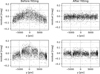 |
Fig. 8. Photometric illumination correction of the weak-lensing THELI data: Flat-fielded OmegaCAM data show systematic zeropoint variations over the field-of-view if the complete mosaic is calibrated with a single photometric zeropoint (left panels). The residuals can well be fitted and corrected with a two-dimensional, second-order polynomial over the field-of-view (right panels). |
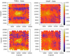 |
Fig. 9. Check of the illumination corrections, through direct comparison of star magnitudes with Gaia. Each panel shows the median difference between a KiDS-DR4 r-magnitude and Gaia-DR2 G-band magnitudes, as a function of (X, Y) position in the focal plane. Stars in the range 18 < r < 19 with 0.7 < (g − i)0 < 1.5 are used, on the flat part of the relation shown in Fig. 6. Top row: results for the tiles in KiDS-N, bottom row: for those in KiDS-S. THELI MAG_AUTO is shown on the left, MAG_GAAP_r on the right. |
Another, more minor, change to the THELI workflow is the streamlining of the procedure for masking residual satellite trails on the single exposures. Whereas previously this was done per CCD, the new procedure allows the inspector to mask the track on the entire mosaic in one step.
4. Single-band u, g, r and i catalogues, images and masks
For every co-added image from the ASTRO-WISE pipeline a single-band catalogue was produced using SEXTRACTOR (Bertin & Arnouts 1996), using the same settings as in DR312. These catalogues are calibrated photometrically using the nightly zeropoints. To convert the fluxes in these catalogues into SLR+Gaia calibrated magnitudes, the zeropoint given in the DMAG keyword should be used. This value should be added to any magnitude found in the catalogue, and any flux in the catalogue can be turned into a magnitude via
 (7)
(7)
The SEXTRACTOR Kron-like MAG_AUTO and isophotal magnitude MAG_ISO are provided, as well as a range of circular-aperture fluxes, star-galaxy classification and shape parameters. Appendix A.1.2 gives a full list of the parameters included in the catalogues. Note that the single-band catalogues are derived independently from each co-added KiDS observation, without cross-calibration or source matching across filter bands. In particular, the sources in the r-band catalogues are extracted from the ASTRO-WISE co-added images, and differ from those in the nine-band catalogue presented below, which are extracted from the THELIr-band images. Also, sources in the overlap region between adjacent tiles will appear in multiple single-band catalogues, with independent measurements for position, flux, etc. The single-band u, g, r and i catalogues contain an average of 22k, 79k, 125k, and 65k sources, respectively, per KiDS tile.
DR4 includes the co-added images with corresponding weight maps and masks, as well as the single-band catalogues described above with SEXTRACTOR output. The PULECENELLA masks identifying stellar reflection haloes are generated in the same way as for DR3, and are described there.
Though it is possible to generate spectral energy distributions by matching the sources in the ugri catalogues for any given tile, it should be remembered that the PSF differs across the bands, and from tile to tile. A better way of obtaining reliable colours is to use the matched-seeing, matched-aperture catalogues described in the next section.
5. The joint KiDS-VIKING nine-band catalogue
Besides more than doubling the area of sky covered with respect to DR3, the major new feature of KiDS-ESO-DR4 is the inclusion of near-infrared fluxes, from the VIKING survey (Edge et al. 2013). This survey was conceived together with KiDS, as a means to improve knowledge of the spectral energy distributions (SEDs) of the sources, and in particular to enhance the quality of the photometric redshift estimates. Because VISTA entered operations before the VST, VIKING was completed first: full coverage of the 1350deg2 area was reached in August of 2016, while repeat observations of low-quality data were completed in February of 201813. DR4 includes photometry for all sources detected on the r-band co-added images as processed with the THELI pipeline: r-band Kron-like MAG_AUTO, isophotal MAG_ISO magnitudes and a range of circular-aperture fluxes, as well as nine-band optical/near-infrared GAAP fluxes for SED estimation. Note that only r-band total magnitudes are supplied.
Full details of the near-IR photometry are presented in Wright et al. (2018). Briefly summarized, the measurements start from the “pawprint” images processed by the Cambridge Astronomical Survey Unit (CASU), which combine each set of jittered observations (offsets of a few arcseconds) into an astrometrically and photometrically calibrated set of sixteen detector-sized images. Each VIKING tile consists of six such pawprints, with observations offset by nearly a full detector width in right ascension, and half that in declination. Because the large gaps between the detectors can result in significant PSF quality jumps after co-addition, the VIKING photometry for KiDS-ESO-DR4 is performed by running the PSF Gaussianization and GAAP separately on each pawprint detector. The final flux in each VISTA band is the optimally weighted average of the individual flux measurements, using the individual flux errors that are derived by propagating the pixel errors (including covariance) through the GAAP procedure as descibed in Appendix A of Kuijken et al. (2015). Due to the VIKING observing strategy sources typically appear on two VIKING pawprints (four in case of J-band), but a few percent of the sources appear six times (twelve in J) or more. The number of exposures that contribute to each source’s VIKING fluxes is given in the catalogue. Note that the optical photometry is performed on the co-added images, which are much less sensitive to PSF changes between sub-exposures because of the very high pixel coverage fraction of the focal plane of the optical camera (which has minimal gaps between the three-edge buttable CCDs in the instrument).
Because of their respective cameras’ different footprints on the sky, KiDS and VIKING tile the sky differently. Data quality variations (depth, seeing, background...) follow a square-degree pattern for the KiDS data, and a 1.5 × 1° pattern for VIKING; moreover within VIKING tiles the variations can be more complex because of the larger gaps between VIRCAM detectors.
The essence of the GAAP photometry (Kuijken et al. 2015) contained in the DR4 nine-band catalogue is to provide accurately aperture-matched fluxes across all wavebands, properly corrected for PSF differences. The aperture major and minor axis lengths, Agaper and Bgaper, are set from the SEXTRACTOR size and shape parameters measured on the detection image, via
 (8)
(8)
(see Fig. 10) with the position angle equal to the position angle THETA_WORLD from the detection image14. As it was in DR3, the MIN_APER parameter is set to  for all sources, and in addition Agaper and Bgaper are maximized at 2″. Imposing a maximum aperture size helps to ensure that the GAAP colours are not contaminated by neighbouring sources, but we do not attempt here to deblend overlapping sources. We note that an explicit flagging of sources affected by neighbours is done by the SEXTRACTOR source detection step, and is also an important part of the forthcoming lensfit shape measurements. For further discussion of the choice of GAAP aperture size, see Kuijken et al. (2015), Appendix A2.
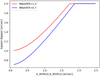 |
Fig. 10. Relation between the SEXTRACTOR major and minor axis measurements (A and B) and the adopted GAAP apertures, for the two minimum aperture (MIN_APER) values that have been used. |
In rare cases, no GAAP flux can be measured with this setup, because GAAP photometry can only be determined when the specified aperture size is larger than the Gaussianized PSF. To provide colours for these sources, DR4 includes a second run with larger apertures, obtained by setting MIN_APER=  . The results from both GAAP runs are present in the catalogues, with keywords whose names contain _0p7 and _1p0 respectively. In general the 1p0 fluxes will have a larger error than those from the standard 0p7 setup, since the larger aperture includes more background noise. However, when the Gaussianized PSF size is close to that of the GAAP aperture, the error increases15; in such cases it may happen that the larger MIN_APER =
  leads to a smaller flux error (and when the PSF is too broad the flux error is formally infinite). In the DR4 catalogue a source-by-source decision is made which optimal MIN_APER choice to use as input for the photometric redshifts, as follows:
-
For all bands x, calculate the flux error ratios
 (9)
(9) -
If
 (10)
(10)
then use the 1p0 fluxes for this source, else adopt 0p7.
This choice ensures that the smaller 0p7 aperture is used, unless there is a band for which the larger aperture gives a smaller flux error, for the reasons indicated above: in that case, the 1p0 fluxes are used if the fractional reduction in the error in that band is greater than the fractional penalty suffered by the other bands16. The larger MIN_APER is preferred in some four percent of the cases. These optimal GAAP fluxes are reported in the catalogue with the FLUX_GAAP_x keywords.
The flux and magnitude zeropoints in the catalogue are as follows.
-
All GAAP fluxes are reported in the units of the image pixel ADU values. For the KiDS images these correspond approximately to a photometric AB magnitude zeropoint of 0; for the VISTA data this zeropoint is 30.
-
The GAAP magnitudes MAG_GAAP_0p7_x and MAG_GAAP_1p0_x for the KiDS ugri bands are calculated from the corresponding fluxes using the zeropoint DMAG_x or DMAG_x_1 (see Sect. 3.1.3) and recorded in the catalogue header.
-
The GAAP magnitudes for the VIKING ZYJHKs bands are calculated with the zeropoint 30.
-
The optimal GAAP fluxes FLUX_GAAP_x are equal to one of the 0p7 or 1p0 sets, as described above.
-
The optimal GAAP magnitudes MAG_GAAP_x are calculated as above, but in addition are also corrected for Galactic extinction by subtracting the EXTINCTION_x value (obtained using the data in Table 4).
-
The colours COLOUR_GAAP_x_y in the catalogue are obtained as differences between these extinction-corrected MAG_GAAP_x magnitudes, and are therefore corrected for Galactic reddening.
The nine-band catalogue also contains those KiDS sources that fall outside the VIKING footprint, as can be seen on the maps of limiting magnitude in Sect. 6.5 below. Note in particular that the COSMOS field near (RA, Dec) =  (KiDS-N-D2 in Table 2) is not part of the VIKING survey, though other – in some cases much deeper – VISTA data do exist for this field. These near-infrared data do not form part of KiDS-DR4, but they are incorporated in the calibration of the photometric redshifts for the KV450 analysis in Hildebrandt et al. (2018).
Figure 11 illustrates the r-band depth and photometric redshift distribution of the sources in the nine-band catalogue. For a list of all columns, see Appendix A.2. The catalogue contains just over 100 million objects.
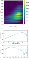 |
Fig. 11. Joint and marginal histograms of the r-band MAG_AUTO magnitude and the Z_B photometric redshift estimate for the sources in the nine-band catalogue. |
6. Data quality
6.1. Image quality
For weak lensing, the most critical science case for KiDS, image quality is a crucial property of the data. KiDS scheduling is designed to take advantage of the periods of excellent seeing on Paranal, by prioritising the r-band exposures at those times. The resulting seeing distribution of the four KiDS bands was shown in Fig. 3.
In Fig. 12 we present maps of the KiDS-ESO-DR4 r-band PSF size and ellipticity, obtained by running the lensfit PSF modelling code used for the KiDS-450 analysis KiDS450 on the THELI images. The top row of the Figure shows the PSF FWHM. Individual KiDS tiles are clearly visible. The second row shows the PSF ellipticity, and the bottom two rows the “1” and “2” ellipticity components. The results of the VST improvements that were implemented in 2015 are reflected in the DR4 data: PSF variations are significantly reduced in the newly added data compared to the data from DR1+2+3 (see the blue areas in Fig. 1).
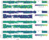 |
Fig. 12. r-band PSF properties across KiDS-ESO-DR4. From top to bottom: FWHM, ellipticity modulus, and ellipticity components 1 and 2 (elongation along the pixel x axis and diagonal, respectively). |
In Fig. 13 we compare the seeing distribution of the KiDS-DR4 r-band data with those of the images used for the lensing measurements in the other major ongoing surveys: the DES-Year 1 riz data (Zuntz et al. 2018), which has a similar depth to KiDS, and the HSC DR1 i-band lensing catalogue (Mandelbaum et al. 2018). The superior seeing of KiDS compared to DES explains why both surveys are providing cosmic shear constraints of comparable power, despite the larger DES area. The impact that can be expected from the complete HSC survey is also evident, even more so considering that it is significantly deeper than KiDS and DES.
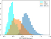 |
Fig. 13. The KiDS r-band seeing FWHM distribution (red) compared to those used for shape measurements in the other major ongoing weak lensing surveys: HSC i band (cyan) and DES r+i+z (blue). |
6.2. Astrometry
The astrometry in the THELI-processed r-band detection images and catalogues is tied to SDSS in the North, and to 2MASS in the South. The ASTRO-WISE images and single-band catalogues are all tied to 2MASS, as is VIKING. Slight differences exist between these two reference catalogues.
We compare the THELI and ASTRO-WISE astrometry to the Gaia DR2 data in Figs. 14 and 15. Systematic residuals between either catalogue and Gaia are at the level of 200 mas; between the THELI and ASTRO-WISE reductions the differences are at most 50 mas. These latter differences are sufficiently small that they will not affect the GAAP photometry (where the apertures are defined on the THELI images, but the fluxes measured at the corresponding positions in the ASTRO-WISE images).
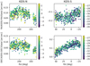 |
Fig. 14. Median THELI astrometry residuals per KiDS tile in the nine-band catalogues, as measured from unsaturated Gaia stars, in arcseconds. Left/right plots: KiDS-N/S, and top and bottom rows: median offsets per tile in RA and Dec. The colours indicate the declination of the tiles, in degrees. |
6.3. Photometry
We assess the accuracy of the KiDS photometric calibration by comparing with overlapping, shallower surveys. For galaxies, comparing the KiDS photometry with catalogues from other surveys is complex, since for extended sources the GAAP fluxes do not measure total fluxes (see Sect. 3.1.2). If desired, the r-band circular aperture fluxes in the catalogue can be used to generate a curve-of growth, and total magnitudes can then be estimated from the GAAP colours. (Alternatively, the r-band MAG_AUTO can be combined with the GAAP colours to generate estimated Kron-like magnitudes in the other bands. Such procedures assume that there are no colour gradients in the galaxy, an assumption that could be tested by comparing the 0p7 and 1p0 GAAP fluxes.)
For stars and other unresolved objects, the situation is different, since their GAAP fluxes are total fluxes: the GAAP flux with Gaussian aperture function ![Mathematical equation: $ W=\exp[-\frac12(x^2/A^2+y^2/B^2)] $](/articles/aa/full_html/2019/05/aa34918-18/aa34918-18-eq37.gif) (in coordinates centered on the source and rotated to align with the aperture major and minor axes) is the integral (on the pre-seeing sky)
(in coordinates centered on the source and rotated to align with the aperture major and minor axes) is the integral (on the pre-seeing sky)
 (11)
(11)
which evaluates to the flux F of the source when the intensity I(x, y) is F times a delta function.
Such a comparison is shown in Fig. 16, for an example tile in KiDS-N where SDSS and KiDS overlap. As expected, the stars form tight sequences close to the line of zero magnitude difference, demonstrating that the KiDS and SDSS zero points are consistent for this tile, while the KiDS GAAP magnitudes of galaxies trail towards fainter magnitudes than the corresponding SDSS magnitude. A similar comparison for the near-IR data is presented in Wright et al. (2018). Tile-by-tile consistency in the four bands, for the KiDS-SDSS overlap, is shown in Fig. 17. The larger scatter in the u band, already discussed in Sect. 3.1.3, is evident, particularly in the fields with higher extinction at the extremes of the RA range. In these tiles there are fewer stars with reliable u band photometry; in addition, because of their lower Galactic latitude the foreground extinction screen approximation is less well justified.
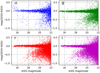 |
Fig. 16. Comparison between the SDSS DR9 model magnitudes and KiDS-ESO-DR4 GAAP photometry. The comparisons are shown for u, g, r, and i bands, for an example tile (KIDS_188.0_−0.5). |
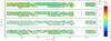 |
Fig. 17. Photometric comparison between KiDS and SDSS photometry of stars in the KiDS-N area. The colourscale indicates the mean magnitude offset mKiDS − mSDSS of high-signal stars u < 20, g < 22, r < 22, i < 20 in every tile. The size of the symbol increases with the FWHM of the PSF. The one outlier in the u-band photometry, tile KIDS_229.0_-2.5_u, is one of the highest-extinction fields in the survey and contains few u-band stars. |
Figure 18 illustrates an internal consistency check of the GAAP magnitudes, that can also serve as a new star-galaxy classifier. The top panel shows the difference between the “0p7” and “1p0” r-band GAAP magnitudes in an example tile. This comparison clearly reveals two populations which are well-separated at the bright end, down to magnitude 22.5. A conservative cut, shown in gold, identifies unresolved objects, for which the GAAP magnitude is independent of aperture size. (Most of the remaining objects are resolved, with higher fluxes for the larger aperture.) The bottom panel shows the location in the g − r, r − i colour–colour diagram of the two populations, confirming that the unresolved objects have mostly stellar colours, whereas the others show the colour distribution expected of a population of galaxies at a wide range of redshifts.
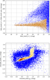 |
Fig. 18. Top plot: star-galaxy separation using the 0p7 and 1p0 GAAP magnitudes. The objects shown in gold form a sequence along which both apertures yield consistent fluxes, indicating that they are unresolved. Bottom plot: g − r, r − i colour–colour diagram for the same sources, confirming that these sources are stars. |
6.4. Photometric redshifts
The nine-band catalogue contains photometric redshift estimates, obtained with the BPZ code (Benítez 2000). It gives the most probable redshift values, as well as the “1σ” 32nd and 68th percentiles of the posterior probability distributions, and the best-fit SED type. The BPZ version and settings are given in Table 5.
Settings for the BPZ photometric redshift calculations.
Since DR3 we have implemented several changes to our photo-z setup. We updated the prior redshift probability used in BPZ to the one given in Raichoor et al. (2014). This prior reduced uncertainties and catastrophic failures for faint galaxies at higher redshifts, but appears to generate a redshift bias for bright, low-redshift galaxies. We therefore caution users of the catalogue to calibrate the BPZ redshifts appropriately before using them. At bright magnitudes, where complete training data are available, it is advantageous to use an empirical photo-z technique like the one presented for the DR3 data set in Bilicki et al. (2018); specific selection and calibration of luminous red galaxies (LRG, Vakili et al. 2018) is also effective. Bright and LRG samples based on DR4 and taking advantage of its unique, deep, nine-band coverage are in preparation.
Another change is related to the photo-z errors and the ODDS quality indicator. In previous releases we reported 95% confidence intervals for the Bayesian redshift estimate. With DR4 we switch to 68% confidence intervals as mentioned above, which requires some changes to the settings and also changes the values of the ODDS parameter. The changes in prior and BPZ settings, together with the fact that we are using full nine-band photometry in a KiDS data release for the first time mean that previous photo-z results based on optical-only photometry (e.g., Kuijken et al. 2015) are no longer advocated.
Further discussion of the nine-band KiDS+VIKING photometric redshifts, as well as a comparison to the KiDS450 photo-z, is provided in Wright et al. (2018) where a similar setup17 was used. There the BPZ photo-z are tested against several deep spectroscopic surveys. At full depth (r ≲ 24.5) the photo-z show a scatter (normalised-median-absolute-deviation) of σm = 0.072 of the quantity Δz/(1 + z)=(zB − zspec)/(1 + zspec) and a fraction ζ0.15 = 17.7% of outliers with |Δz/(1 + z)| ≥ 0.15. The magnitude dependence of these quantities is shown in Fig. 19. The effect of the different selection criteria in the spectroscopic catalogues is evident (e.g., the bump in the redshift bias μΔz near r = 18, which marks the transition from the BOSS LOWZ to CMASS samples), illustrating that calibrating the photometric redshift error distribution requires care (see Bilicki et al. 2018 and the extensive discussion of direct calibration techniques in KiDS450 for further details). Note also that the photo-z setup was optimised for the fainter, r > 20 galaxies that are of interest for the KiDS cosmology analysis, and not for the brighter galaxies.
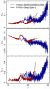 |
Fig. 19. r-Magnitude dependence of KiDS DR4 photo-z statistics based on the findings of Wright et al. (2018) for the deep spec-z fields (blue lines) and a direct comparison of DR4 photo-z and SDSS/2dFLenS spec-z (red lines). Top panel: normalised-median-absolute-deviation of the quantity Δz/(1 + z), middle panel: mean μΔz of that quantity, and lower panel: rate ζ0.15 of outliers with |Δz/(1 + z)| ≥ 0.15. (Note that this definition of ζ0.15 exaggerates the outlier fraction when σm approaches 0.1.) The scatter between neighbouring points gives an indication of the error bars on these quantities. |
6.5. Photometric depth and homogeneity
Figure 20 shows the distribution of the different bands’ 1σ limiting magnitudes in the catalogue. Note the narrow range of the limiting magnitudes in the u, g, and particularly the r band, a consequence of the KiDS observing strategy of choosing which dark-time band to observe in according to the seeing conditions. Maps of the median limiting magnitude in  cells are presented in Fig. 21 (KiDS ugri) and 22 (VIKING ZYJHKs).
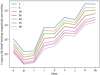 |
Fig. 20. Various percentiles of the 1σ GAAP limiting magnitudes for the nine wavelength bands. The width of the distributions is driven by differences in seeing, air mass and sky brightness across the KiDS and VIKING surveys. |
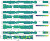 |
Fig. 21. Maps of the median limiting GAAP magnitude, corresponding to the 1σ flux error, in |

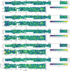 |
Fig. 22. Maps of the r-band selected sources’ median limiting GAAP magnitude, corresponding to the 1σ flux error, in |


7. Data access
There are several ways through which KiDS-ESO-DR4 data products can be accessed. An overview is presented in this section and up-to-date information is also available at the KiDS DR4 website.
The data products that constitute the DR4 release (stacked ugri images and their associated weight maps, flag maps, and single-band source lists for 1006 survey tiles, the r-band detection images and their weight maps, as well as the multi-band catalog combining KiDS and VIKING photometry together with flag maps combining mask information from all filters), are released via the ESO Science Archive, and also accessible via ASTRO-WISE and the KiDS website.
7.1. ESO science archive
All main release data products are disseminated through the ESO Science Archive Facility18, which provides several interfaces and query forms. All image stacks, weight maps, flag maps and single-band source lists are provided on a per tile basis via the “Phase 3 main query form”. This interface supports queries on several parameters, including position, object name, filter, observation date, etc. and allows download of the tile-based data files. Also the multi-band catalog, which is stored in per-tile data files, is available in this manner. A more advanced method to query the multi-band catalog is provided by the “Catalogue Facility query interface”, which enables users to perform queries on any of the catalog columns, for example facilitating selections based on area, magnitude, photo-z or shape information. Finally, data can be queried directly from a new graphical sky projection interface known as the “Science Portal”. Query results can subsequently be exported to various (single-file) formats.
7.2. ASTRO-WISE archive
Most of the data products can also be retrieved from the ASTRO-WISE system (Begeman et al. 2013). This data processing and management system is used for the production of these data products and retains the full data lineage. For scientists interested in access to various quality controls, further analysis tools, or reprocessing of data this access route may be convenient. The DBviewer web service19 allows querying for data products and supports file downloads, viewing of inspection plots, and data lineage browsing. Links with DBviewer queries to complete sets of data products are compiled on the KiDS DR4 website. Several data products that are not in the ESO archive may be retrieved through this route: most importantly, the PSF-Gaussianized images and the individual CCD sub-exposures after various stages of processing in the ASTRO-WISE pipeline are available here.
7.3. KiDS DR4 website
Apart from offering an up-to-date overview of all data access routes, the KiDS DR4 website20 also provides alternative ways for data retrieval and quality control.
The synoptic table presents for each observation (tile/filter) a combination of inspection plots relating to the image and source extraction quality, as well as links for direct downloads of the various data FITS files. Furthermore, direct batch downloads of all DR4 FITS files are supported by supplying WGET scripts.
8. Summary and outlook
With the KiDS-ESO-DR4 data release, data for over 1000 square degrees, more than two thirds of the target KiDS footprint, is now publicly available. Co-added images with associated weights and masks, as well as single-band source catalogues, may now be accessed through the ESO archive or the KiDS project website.
Moreover, through a combined analysis of these KiDS images with data from the VIKING survey, a nine-band matched-aperture u–Ks catalogue containing some 100 million galaxies has been created, with limiting 5σ AB magnitudes ranging from ca. 25 in g and r bands to 23 in J and 22 in Ks (Fig. 20). This data set is by far the largest-area optical+near-IR data set to this depth. The galaxies in this catalogue have been detected using a reduction of the data that has been optimised for weak gravitational lensing measurements, to enable the primary science goal of KiDS. The GAAP photometry in the nine-band catalogue uses the positions and sizes of these galaxies to define the apertures. Analysis of the gravitational lensing information in the data set is in progress, and shear estimates for these sources will be released in due course. Photometric redshift estimates based on the nine-band photometry are already included in the DR4 catalogue (but see Sect. 6.4 for a discussion of redshift biases for bright sources).
Multiple other applications of this unique optical+near-infrared catalogue are foreseen. For example, stellar mass estimates for galaxies will benefit greatly from the inclusion of the near-IR fluxes (Wright et al. 2018), red-sequence cluster searches can be pushed to greater redshift, and star-galaxy separation and galaxy SED typing can be made more accurate as well (e.g., Daddi et al. 2004; Tortora et al. 2018b).
The data processing for DR4 largely followed the procedures established for the previous data release as described in DR3, with a few improvements:
-
this is the first KiDS data release for which the photometry has been tied to the Gaia database;
-
satellite tracks and other artefacts are now masked at the sub-exposure level, increasing the usable area of the co-added images;
-
the PSF Gaussianization procedure now operates in pixel space, solving directly for a double-shapelet convolution kernel that renders the PSF Gaussian;
-
extinction corrections have been updated to the Schlafly & Finkbeiner (2011) extinction coefficients;
-
GAAP photometry is run twice, with the second run using larger apertures to be able to include occasional poor-seeing KiDS or VIKING data in the photometry catalogue;
-
the THELI processing of the images on which the sources for the nine-band catalogue are detected now includes an illumination correction;
-
the inclusion of the VIKING data involved a re-reduction of the VIKING paw-print level data (see Wright et al. 2018), and is the first time the PSF Gaussianization and GAAP photometry have been performed at sub-exposure level and combined.
The data are publicly available via the ESO archive, the ASTRO-WISE system, and the KiDS project website. A description of the data format may be found in the Appendix.
KiDS observations continue, and are expected to wind down by the middle of 2019, at which point some 1350 square degrees will have been mapped in 9 photometric bands by the combined KiDS+VIKING project.
A repeat pass of the whole survey area in the i-band is also close to completion. These data will enable variability studies on timescales of several years, as well as improving the overall quality of the i-band data, which has the greatest variation in observing conditions and cosmetic quality. In addition, a number of fields with deep spectroscopic redshifts are also being targeted with the VST and VISTA to provide KiDS+VIKING-like photometry for large samples of faint galaxies that can be used as redshift calibrators.
The next full data release, DR5, is expected to be the final one, containing data from the full KiDS/VIKING footprint shown in Fig. 1. Intermediate “value-added” public releases based on DR4, including one with weak lensing shape measurements, will be made together with the corresponding scientific analyses.
The originally planned KiDS area was 1500 square degrees, but this was reduced to match the footprint of the VIKING area.
Note that for DR4 there is no separate multi-band catalogue based on r-band detections in the ASTRO-WISE data, as there was for DR3.
We have found the 2MASS catalogue to be sufficient as astrometric reference, but intend to move to Gaia in the future.
Note that the Gaia DR2 g-band calibration differs from what was used in Gaia DR1, through a new determination of the filter bandpass.
The earlier data releases used the Schlegel et al. (1998) coefficients.
Note that the SEXTRACTOR settings are optimised for small sources; measurements for large objects such as extended galaxies should be used with care because of possible shredding or oversubtraction of the background (e.g., Kelvin et al. 2018).
The VIKING repeat observations taken by September 26, 2016 are incorporated into the DR4 catalogues presented here.
The convention in the GAAP code is that the position angle is measured from East to North, so the catalogue contains the angle PA_GAAP = 180−THETA_WORLD.
Because the aperture that is used for the photometry is the GAAP aperture deconvolved by the PSF.
This formulation also handles the convention that an unmeasured GAAP flux returns an error of −1, provided the rare cases that a 1p0 flux cannot be measured but a 0p7 flux can, are caught.
The main difference of the DR4 setup is the implementation of two different minimum aperture sizes as discussed in Sect. 5. As this change only impacts data with seeing that greatly varies between bands in Wright et al. (2018), it does not affect the photo-z statistics presented here.
Acknowledgments
We are indebted to the staff at ESO-Garching and ESO-Paranal for managing the observations at VST and VISTA that yielded the data presented here. Based on observations made with ESO Telescopes at the La Silla Paranal Observatory under programme IDs 177.A-3016, 177.A-3017, 177.A-3018 and 179.A-2004, and on data products produced by the KiDS consortium. The KiDS production team acknowledges support from: Deutsche Forschungsgemeinschaft, ERC, NOVA and NWO-M grants; Target; the University of Padova, and the University Federico II (Naples). Data processing for VIKING has been contributed by the VISTA Data Flow System at CASU, Cambridge and WFAU, Edinburgh. This work is supported by the Deutsche Forschungsgemeinschaft in the framework of the TR33 ‘The Dark Universe’. We acknowledge support from European Research Council grants 647112 (CH, BG) and 770935 (HHi), the Deutsche Forschungsgemeinschaft (HHi, Emmy Noether grant Hi 1495/2-1 and Heisenberg grant Hi 1495/5-1), the Polish Ministry of Science and Higher Education (MB, grant DIR/WK/2018/12), the INAF PRIN-SKA 2017 program 1.05.01.88.04 (CT), the Alexander von Humboldt Foundation (KK), the STFC (LM, grant ST/N000919/1), and NWO (KK, JdJ, MB, HHo, research grants 621.016.402, 614.001.451 and 639.043.512). We are very grateful to the Lorentz Centre and ESO-Garching for hosting several team meetings. Author contributions: All authors contributed to the work presented in this paper. The author list consists of three groups. The seven lead authors headed various aspects of the data processing. The second group (listed alphabetically) provided significant effort to the production of DR4. The third group contributed to the processing and quality control inspection to a lesser extent, or provided significant input to the paper.
References
- Aihara, H., Arimoto, N., Armstrong, R., et al. 2018, PASJ, 70, S4 [NASA ADS] [Google Scholar]
- Alam, S., Albareti, F. D., Allende Prieto, C., et al. 2015, ApJS, 219, 12 [NASA ADS] [CrossRef] [Google Scholar]
- Amaro, V., Cavuoti, S., Brescia, M., et al. 2019, MNRAS, 482, 3116 [NASA ADS] [CrossRef] [Google Scholar]
- Amon, A., Blake, C., Heymans, C., et al. 2018, MNRAS, 479, 3422 [NASA ADS] [CrossRef] [Google Scholar]
- Asgari, M., Heymans, C., Hildebrandt, H., et al. 2019, A&A, 624, A134 [NASA ADS] [CrossRef] [EDP Sciences] [Google Scholar]
- Begeman, K., Belikov, A. N., Boxhoorn, D. R., & Valentijn, E. A. 2013, Exp. Astron., 35, 1 [NASA ADS] [Google Scholar]
- Bellagamba, F., Sereno, M., Roncarelli, M., et al. 2019, MNRAS, 484, 1598 [NASA ADS] [CrossRef] [Google Scholar]
- Benítez, N. 2000, ApJ, 536, 571 [NASA ADS] [CrossRef] [Google Scholar]
- Bertin, E. 2006, in Astronomical Data Analysis Software and Systems XV, eds. C. Gabriel, C. Arviset, D. Ponz, & S. Enrique, ASP Conf. Ser., 351, 112 [NASA ADS] [Google Scholar]
- Bertin, E. 2010a, Astrophysics Source Code Library [record ascl:1010.063] [Google Scholar]
- Bertin, E. 2010b, Astrophysics Source Code Library [record ascl:1010.068] [Google Scholar]
- Bertin, E., & Arnouts, S. 1996, A&AS, 117, 393 [NASA ADS] [CrossRef] [EDP Sciences] [Google Scholar]
- Bertin, E., Mellier, Y., Radovich, M., et al. 2002, in Astronomical Data Analysis Software and Systems XI, eds. D. A. Bohlender, D. Durand, & T. H. Handley, ASP Conf. Ser., 281, 228 [NASA ADS] [Google Scholar]
- Bilicki, M., Hoekstra, H., Brown, M. J. I., et al. 2018, A&A, 616, A69 [NASA ADS] [CrossRef] [EDP Sciences] [Google Scholar]
- Brouwer, M. M., Cacciato, M., Dvornik, A., et al. 2016, MNRAS, 462, 4451 [NASA ADS] [CrossRef] [Google Scholar]
- Brouwer, M. M., Demchenko, V., Harnois-Déraps, J., et al. 2018, MNRAS, 481, 5189 [NASA ADS] [CrossRef] [Google Scholar]
- Brown, A. G. A., Vallenari, A., Prusti, T., et al. 2018, A&A, 616, A1 [NASA ADS] [CrossRef] [EDP Sciences] [Google Scholar]
- Capaccioli, M., & Schipani, P. 2011, The Messenger, 146, 2 [NASA ADS] [Google Scholar]
- Capaccioli, M., Schipani, P., De Paris, G., et al. 2012, Science from the Next Generation Imaging and Spectroscopic Surveys, 1 [Google Scholar]
- Costa-Duarte, M. V., Viola, M., Molino, A., et al. 2018, MNRAS, 478, 1968 [NASA ADS] [Google Scholar]
- Daddi, E., Cimatti, A., Renzini, A., et al. 2004, ApJ, 617, 746 [NASA ADS] [CrossRef] [Google Scholar]
- Dark Energy Survey Collaboration 2005, ArXiv e-prints [arXiv:astro-ph/0510346] [Google Scholar]
- de Jong, J. T. A., Kuijken, K., Applegate, D., et al. 2013, The Messenger, 154, 44 [NASA ADS] [Google Scholar]
- de Jong, J. T. A., Verdoes Kleijn, G. A., Boxhoorn, D. R., et al. 2015, A&A, 582, A62 (DR1/2) [NASA ADS] [CrossRef] [EDP Sciences] [Google Scholar]
- de Jong, J. T. A., Verdoes Kleijn, G. A., Erben, T., et al. 2017, A&A, 604, A134 (DR3) [NASA ADS] [CrossRef] [EDP Sciences] [Google Scholar]
- Driver, S. P., Hill, D. T., Kelvin, L. S., et al. 2011, MNRAS, 413, 971 [NASA ADS] [CrossRef] [Google Scholar]
- Dvornik, A., Hoekstra, H., Kuijken, K., et al. 2018, MNRAS, 479, 1240 [NASA ADS] [CrossRef] [Google Scholar]
- Edge, A., Sutherland, W., Kuijken, K., et al. 2013, The Messenger, 154, 32 [NASA ADS] [Google Scholar]
- Erben, T., Schirmer, M., Dietrich, J. P., et al. 2005, Astron. Nachr., 326, 432 [NASA ADS] [CrossRef] [Google Scholar]
- Georgiou, C., Johnston, H., Hoekstra, H., et al. 2019, A&A, 622, A90 [NASA ADS] [CrossRef] [EDP Sciences] [Google Scholar]
- Giblin, B., Heymans, C., Harnois-Déraps, J., et al. 2018, MNRAS, 480, 5529 [NASA ADS] [CrossRef] [Google Scholar]
- Harnois-Déraps, J., Tröster, T., Chisari, N. E., et al. 2017, MNRAS, 471, 1619 [NASA ADS] [CrossRef] [Google Scholar]
- Hikage, C., Oguri, M., Hamana, T., et al. 2019, PASJ, 71, 43 [NASA ADS] [CrossRef] [Google Scholar]
- Hildebrandt, H., Erben, T., Kuijken, K., et al. 2012, MNRAS, 421, 2355 [NASA ADS] [CrossRef] [Google Scholar]
- Hildebrandt, H., Viola, M., Heymans, C., et al. 2017, MNRAS, 465, 1454 (KiDS450) [Google Scholar]
- Hildebrandt, H., Köhlinger, F., van den Busch, J. L., et al. 2018, A&A, submitted [arXiv:1812.06076] [Google Scholar]
- Ivezić, Ž., Lupton, R. H., Schlegel, D., et al. 2004, Astron. Nachr., 325, 583 [NASA ADS] [CrossRef] [Google Scholar]
- Jakobs, A., Viola, M., McCarthy, I., et al. 2018, MNRAS, 480, 3338 [NASA ADS] [CrossRef] [Google Scholar]
- Johnston, H., Georghiou, C., Hoekstra, H., et al. 2019, A&A, 624, A30 [NASA ADS] [CrossRef] [EDP Sciences] [Google Scholar]
- Joudaki, S., Mead, A., Blake, C., et al. 2017, MNRAS, 471, 1259 [NASA ADS] [CrossRef] [Google Scholar]
- Kelvin, L. S., Bremer, M. N., Phillipps, S., et al. 2018, MNRAS, 477, 4116 [NASA ADS] [CrossRef] [Google Scholar]
- Köhlinger, F., Viola, M., Joachimi, B., et al. 2017, MNRAS, 471, 4412 [NASA ADS] [CrossRef] [Google Scholar]
- Kuijken, K. 2011, The Messenger, 146, 8 [NASA ADS] [Google Scholar]
- Kuijken, K., Heymans, C., Hildebrandt, H., et al. 2015, MNRAS, 454, 3500 [NASA ADS] [CrossRef] [Google Scholar]
- Laureijs, R., Amiaux, J., Arduini, S., et al. 2011, ArXiv e-prints [arXiv:1110.3193] [Google Scholar]
- Mahlke, M., Bouy, H., Altieri, B., et al. 2018, A&A, 610, A21 [NASA ADS] [CrossRef] [EDP Sciences] [Google Scholar]
- Mandelbaum, R., Miyatake, H., Hamana, T., et al. 2018, PASJ, 70, S25 [NASA ADS] [CrossRef] [Google Scholar]
- Martinet, N., Schneider, P., Hildebrandt, H., et al. 2018, MNRAS, 474, 712 [NASA ADS] [CrossRef] [Google Scholar]
- Maturi, M., Bellagamba, F., Radovich, M., et al. 2019, MNRAS, 485, 498 [NASA ADS] [CrossRef] [Google Scholar]
- McFarland, J. P., Verdoes-Kleijn, G., Sikkema, G., et al. 2013, Exp. Astron., 35, 45 [NASA ADS] [CrossRef] [Google Scholar]
- Nakoneczny, S., Bilicki, M., Solarz, A., et al. 2019, A&A, 624, A13 [NASA ADS] [CrossRef] [EDP Sciences] [Google Scholar]
- Petrillo, C. E., Tortora, C., Chatterjee, S., et al. 2019, MNRAS, 482, 807 [NASA ADS] [Google Scholar]
- Planck Collaboration VI. 2018, A&A, submitted [arXiv:1807.06209] [Google Scholar]
- Raichoor, A., Mei, S., Erben, T., et al. 2014, ApJ, 797, 102 [NASA ADS] [CrossRef] [Google Scholar]
- Roy, N., Napolitano, N. R., La Barbera, F., et al. 2018, MNRAS, 480, 1057 [NASA ADS] [CrossRef] [Google Scholar]
- Schlafly, E. F., & Finkbeiner, D. P. 2011, ApJ, 737, 103 [NASA ADS] [CrossRef] [Google Scholar]
- Schlegel, D. J., Finkbeiner, D. P., & Davis, M. 1998, ApJ, 500, 525 [NASA ADS] [CrossRef] [Google Scholar]
- Sergeyev, A., Spiniello, C., Khramtsov, V., et al. 2018, Res. Notes Am. Astron. Soc., 2, 189 [Google Scholar]
- Shan, H., Liu, X., Hildebrandt, H., et al. 2018, MNRAS, 474, 1116 [NASA ADS] [CrossRef] [Google Scholar]
- Sifón, C., Cacciato, M., Hoekstra, H., et al. 2015, MNRAS, 454, 3938 [NASA ADS] [CrossRef] [Google Scholar]
- Skrutskie, M. F., Cutri, R. M., Stiening, R., et al. 2006, AJ, 131, 1163 [NASA ADS] [CrossRef] [Google Scholar]
- Spergel, D., Gehrels, N., Baltay, C., et al. 2015, ArXiv e-prints [arXiv:1503.03757] [Google Scholar]
- Spiniello, C., Agnello, A., Napolitano, N. R., et al. 2018, MNRAS, 480, 1163 [NASA ADS] [CrossRef] [Google Scholar]
- Tortora, C., Napolitano, N. R., Roy, N., et al. 2018a, MNRAS, 473, 969 [NASA ADS] [CrossRef] [Google Scholar]
- Tortora, C., Napolitano, N. R., Spavone, M., et al. 2018b, MNRAS, 481, 4728 [NASA ADS] [CrossRef] [Google Scholar]
- Troxel, M. A., MacCrann, N., Zuntz, J., et al. 2018, Phys. Rev. D, 98, 043528 [NASA ADS] [CrossRef] [Google Scholar]
- Vakili, M., Bilicki, M., Hoekstra, H., et al. 2018, ArXiv e-prints [arXiv:1811.02518] [Google Scholar]
- van Uitert, E., Cacciato, M., Hoekstra, H., et al. 2016, MNRAS, 459, 3251 [NASA ADS] [CrossRef] [Google Scholar]
- van Uitert, E., Hoekstra, H., Joachimi, B., et al. 2017, MNRAS, 467, 4131 [NASA ADS] [CrossRef] [Google Scholar]
- van Uitert, E., Joachimi, B., Joudaki, S., et al. 2018, MNRAS, 476, 4662 [NASA ADS] [CrossRef] [Google Scholar]
- Viola, M., Cacciato, M., Brouwer, M., et al. 2015, MNRAS, 452, 3529 [CrossRef] [Google Scholar]
- Wright, A. H., Hildebrandt, H., Kuijken, K., et al. 2018, A&A, submitted [arXiv:1812.06077] [Google Scholar]
- Zuntz, J., Sheldon, E., Samuroff, S., et al. 2018, MNRAS, 481, 1149 [NASA ADS] [CrossRef] [Google Scholar]
Appendix A: Description of the data products
The data release consists of single-band data products, based on individual KiDS tiles observed with the u, g, r and i filters and processed with ASTRO-WISE, as well as a multi-band sourcelist with photometry in 9 bands for sources detected in r, the deepest KiDS band. The r-band images used for this latter source list result from a separate reduction of the KiDS images, using THELI, that is optimised for weak lensing measurements. There are therefore differences between the single-band r catalogues and the multi-band source lists. The nine-band catalogue can be queried via the ESO archive interface, or downloaded as separate fits tables per survey tile. Shape parameters for the sources in the nine-band catalogue will be released as part of the upcoming KiDS-DR4 weak lensing analysis.
File names for the various products follow the scheme given in Table A.1.
A.1. Single-band data products
A.1.1. Co-added images
For each of the 1006 survey tiles, we provide a co-added image in each of the four KiDS filters. Image names are of the form KiDS_DR4.0_RA_DEC_x_sci.fits, where RA and Dec are the nominal central coordinates of the tile, in degrees rounded to the nearest tenth, and x is the filter. Images are regridded to a grid of  pixels, using a tangential projection. The images are background-subtracted. Associated inverse-variance weight images are also provided (*_wei.fits) as well as automatically generated pixel bitmasks (*_msk.fits). Different bits in the flag values indicate different types of issues: 1 = readout spike; 2 = saturation core; 4 = diffraction spike; 8 = primary reflection halo; 16 = secondary reflection halo; 32 = tertiary reflection halo; 64 = bad pixel. Several pertinent keywords that can be found in the headers of these ASTRO-WISE images are listed in Table A.2.
The THELI versions of the r-band images are also provided. These co-added images and weight file have names that contain the “_det_” string (Table A.1), to indicate that they are the detection images for the list-driven multi-band photometry.
A.1.2. Source lists
Corresponding to each single-band co-added image, DR4 provides a source list KiDS_DR4.0_[RA]_[DEC]_x_src.fits, with columns as listed in Table A.3. Note that the single-band catalogues include all sources detected in each observation, including ones near the edge of the field that also fall on one or more other tiles. The structure of these catalogues is the same as it was in DR3, but we repeat the description here for completeness. More information on some of the columns is provided below:
-
2DPHOT: KIDS-CAT star/galaxy classification bitmap based on the source morphology (see de Jong et al. 2015). Values are: 1 = high confidence star candidate; 2 = unreliable source (e.g. cosmic ray); 4 = star according to star/galaxy separation criteria; 0 = all other sources (e.g. including galaxies). Sources identified as stars can thus have a flag value of 1, 4 or 5.
-
IMAFLAGS_ISO: A bitmap of the mask flags (see Sect. A.1.1) that are set anywhere within the source’s isophote.
-
FLUX_APER_* and FLUXERR_APER_* : aperture flux measurements are included for 27 different aperture sizes. In Table A.3 only the smallest (2 pixels or
 diameter) and the largest (200 pixels or 40″ diameter) are listed; the label for the aperture of 28.5 pixels is FLUX_APER_28p5.
The header of the SOURCELIST extension of these fits files contains the ABMAGLIM, PSF_FWHM, ELLIPTIC, CALSTARS, DMAG and CALMINAP keywords inherited from the corresponding science image (see Table A.2).
A.2. Nine-band catalogue
The production of the nine-band catalogues is described in Sect. 5. The data release consists of 1006 catalogues one per KiDS tile. The catalogues have been cut in right ascension and declination at the edges of the fields to prevent duplication of sources in neighbouring tiles, so that the catalogues fit together seamlessly. The cuts are based on the KiDS survey pattern. Since the VIKING survey uses an instrument with a different footprint on the sky, different VIKING survey tiles generally contribute to the data for a single catalogue.
The nine-band catalogue files are called KiDS_DR4.0_[RA]_[DEC]_ugriZYJHKs_cat.fits. The columns in the nine-band catalogues are described in Table A.4. The nine-band catalogues’ MASK column is a combination of the mask values of the single-band observations, and its meaning is given in Table A.5. They should not be confused with the MASK flags in the single-band catalogues.
In addition, the header of each catalogue contains keywords that reference the KiDS input data sets. The most pertinent of these are listed in Table A.6.
File names for the data products associated with each KiDS tile.
Most important header keywords in the ASTRO-WISE “*sci.fits” images
Columns provided in the single-band source lists.
Columns provided in the nine-band catalogue.
Bit values of the nine-band MASK parameter.
Main keywords in the nine-band catalogue headers.
All Tables
Extinction coefficients Rf = Af/E(B − V) used in this work, from Schlafly & Finkbeiner (2011; SF11).
All Figures
|
Fig. 1. Sky distribution of survey tiles released in KiDS-ESO-DR4. Tiles shown in green are released for the first time; those in blue were included in the earlier data releases (DR1+2+3) but have been reprocessed for DR4. The full KiDS+VIKING area (∼1350deg2) is shown in grey. Top: KiDS-North. Bottom: KiDS-South. The single pointing at RA = 150deg is centred on the COSMOS/CFHTLS D2 field. |
| In the text | |
|
Fig. 2. Progress of the KiDS observations at the VST, in the four survey bands. Each Observing Block (OB) produces a square-degree co-added image. The i-band data, for which data taking was significantly faster because of less competition for bright time on the telescope, had covered the originally planned 1500 square degree footprint by the time it was decided to limit the survey to the 1350 square degree area that comprise the completed VIKING area. The dashed lines indicate the cutoff dates for KiDS-ESO data releases 1–4. |
| In the text | |
|
Fig. 3. Distributions of tile-by-tile data quality parameters for the KiDS DR4 data, grouped by filter, from top to bottom u, g, r and i. The light-coloured histograms represent the subset of the data that was previously released in DR1+2+3. Left: seeing. The differences between the bands reflect the observing strategy of reserving the best-seeing dark time for r-band observations. Middle column: average PSF ellipticity ⟨|epsf|⟩, where e is defined as 1 − b/a for major/minor axis lengths a and b. Right: limiting AB magnitude (5σ in a 2″ aperture). The wider distribution of the i-band observations is a caused by variations in the moon illumination, since the i-band data were mostly taken in bright time. |
| In the text | |
|
Fig. 4. Schematic representation of the DR4 processing steps and content. Yellow boxes show the input data from VST and VISTA, green indicates image products, and source lists are shown in pink. The lensfit-based lensing measurements – initially not released in DR4 – are shown as dotted lines. |
| In the text | |
|
Fig. 5. Residual u-band magnitude variation when Eq. (3) is used without a dependence on Galactic latitude b (i.e., f(b)=0). Each point shows the average offset uKiDS − uSDSS for the calibration stars in a separate KiDS-N tile. The line represents the Galactic latitude correction of Eq. (4). |
| In the text | |
|
Fig. 6. Colour–colour relation used to calibrate the KiDS r-band measurements to the Gaia G-band catalogue, for an example tile. The blue points and the box indicate the dereddened (g − i) colour range for the stars used, and the ±0.05 mag iterative clipping width about the fiducial sequence. The shape of the sequence is determined from the overlap area between KiDS-N and SDSS. |
| In the text | |
|
Fig. 7. Distribution of the u, g, r and i zeropoint corrections using the stellar locus regression plus Gaia calibration. |
| In the text | |
|
Fig. 8. Photometric illumination correction of the weak-lensing THELI data: Flat-fielded OmegaCAM data show systematic zeropoint variations over the field-of-view if the complete mosaic is calibrated with a single photometric zeropoint (left panels). The residuals can well be fitted and corrected with a two-dimensional, second-order polynomial over the field-of-view (right panels). |
| In the text | |
|
Fig. 9. Check of the illumination corrections, through direct comparison of star magnitudes with Gaia. Each panel shows the median difference between a KiDS-DR4 r-magnitude and Gaia-DR2 G-band magnitudes, as a function of (X, Y) position in the focal plane. Stars in the range 18 < r < 19 with 0.7 < (g − i)0 < 1.5 are used, on the flat part of the relation shown in Fig. 6. Top row: results for the tiles in KiDS-N, bottom row: for those in KiDS-S. THELI MAG_AUTO is shown on the left, MAG_GAAP_r on the right. |
| In the text | |
|
Fig. 10. Relation between the SEXTRACTOR major and minor axis measurements (A and B) and the adopted GAAP apertures, for the two minimum aperture (MIN_APER) values that have been used. |
| In the text | |
|
Fig. 11. Joint and marginal histograms of the r-band MAG_AUTO magnitude and the Z_B photometric redshift estimate for the sources in the nine-band catalogue. |
| In the text | |
|
Fig. 12. r-band PSF properties across KiDS-ESO-DR4. From top to bottom: FWHM, ellipticity modulus, and ellipticity components 1 and 2 (elongation along the pixel x axis and diagonal, respectively). |
| In the text | |
|
Fig. 13. The KiDS r-band seeing FWHM distribution (red) compared to those used for shape measurements in the other major ongoing weak lensing surveys: HSC i band (cyan) and DES r+i+z (blue). |
| In the text | |
|
Fig. 14. Median THELI astrometry residuals per KiDS tile in the nine-band catalogues, as measured from unsaturated Gaia stars, in arcseconds. Left/right plots: KiDS-N/S, and top and bottom rows: median offsets per tile in RA and Dec. The colours indicate the declination of the tiles, in degrees. |
| In the text | |
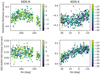 |
Fig. 15. As Fig. 14, but for the ASTRO-WISE single-band r catalogues. |
| In the text | |
|
Fig. 16. Comparison between the SDSS DR9 model magnitudes and KiDS-ESO-DR4 GAAP photometry. The comparisons are shown for u, g, r, and i bands, for an example tile (KIDS_188.0_−0.5). |
| In the text | |
|
Fig. 17. Photometric comparison between KiDS and SDSS photometry of stars in the KiDS-N area. The colourscale indicates the mean magnitude offset mKiDS − mSDSS of high-signal stars u < 20, g < 22, r < 22, i < 20 in every tile. The size of the symbol increases with the FWHM of the PSF. The one outlier in the u-band photometry, tile KIDS_229.0_-2.5_u, is one of the highest-extinction fields in the survey and contains few u-band stars. |
| In the text | |
|
Fig. 18. Top plot: star-galaxy separation using the 0p7 and 1p0 GAAP magnitudes. The objects shown in gold form a sequence along which both apertures yield consistent fluxes, indicating that they are unresolved. Bottom plot: g − r, r − i colour–colour diagram for the same sources, confirming that these sources are stars. |
| In the text | |
|
Fig. 19. r-Magnitude dependence of KiDS DR4 photo-z statistics based on the findings of Wright et al. (2018) for the deep spec-z fields (blue lines) and a direct comparison of DR4 photo-z and SDSS/2dFLenS spec-z (red lines). Top panel: normalised-median-absolute-deviation of the quantity Δz/(1 + z), middle panel: mean μΔz of that quantity, and lower panel: rate ζ0.15 of outliers with |Δz/(1 + z)| ≥ 0.15. (Note that this definition of ζ0.15 exaggerates the outlier fraction when σm approaches 0.1.) The scatter between neighbouring points gives an indication of the error bars on these quantities. |
| In the text | |
|
Fig. 20. Various percentiles of the 1σ GAAP limiting magnitudes for the nine wavelength bands. The width of the distributions is driven by differences in seeing, air mass and sky brightness across the KiDS and VIKING surveys. |
| In the text | |
|
Fig. 21. Maps of the median limiting GAAP magnitude, corresponding to the 1σ flux error, in |
| In the text | |
|
Fig. 22. Maps of the r-band selected sources’ median limiting GAAP magnitude, corresponding to the 1σ flux error, in |
| In the text | |
Current usage metrics show cumulative count of Article Views (full-text article views including HTML views, PDF and ePub downloads, according to the available data) and Abstracts Views on Vision4Press platform.
Data correspond to usage on the plateform after 2015. The current usage metrics is available 48-96 hours after online publication and is updated daily on week days.
Initial download of the metrics may take a while.