| Issue |
A&A
Volume 624, April 2019
|
|
|---|---|---|
| Article Number | A50 | |
| Number of page(s) | 12 | |
| Section | Stellar structure and evolution | |
| DOI | https://doi.org/10.1051/0004-6361/201834342 | |
| Published online | 10 April 2019 | |
New view of the corona of classical T Tauri stars: Effects of flaring activity in circumstellar disks⋆
1
Dipartimento di Fisica & Chimica Specola Universitaria, Università degli Studi di Palermo, Piazza del Parlamento 1, 90143 Palermo, Italy
e-mail: scolombo@astropa.unipa.it
2
LERMA, Observatoire de Paris, Sorbonne Université, Université PSL, CNRS, Paris, France
3
INAF-Osservatorio Astronomico di Palermo “G.S. Vaiana”, Piazza del Parlamento 1, 90134 Palermo, Italy
Received:
28
September
2018
Accepted:
19
February
2019
Context. Classical T Tauri stars (CTTSs) are young low-mass stellar objects that accrete mass from their circumstellar disks. They are characterized by high levels of coronal activity, as revealed by X-ray observations. This activity may affect the disk stability and the circumstellar environment.
Aims. Here we investigate if an intense coronal activity due to flares that occur close to the accretion disk may perturb the stability of the inner disk, disrupt the inner part of the disk, and might even trigger accretion phenomena with rates comparable with those observed.
Methods. We modeled a magnetized protostar surrounded by an accretion disk through 3D magnetohydrodinamic simulations. The model takes into account the gravity from the central star, the effects of viscosity in the disk, the thermal conduction (including the effects of heat flux saturation), the radiative losses from optically thin plasma, and a parameterized heating function to trigger the flares. We explored cases characterized by a dipole plus an octupole stellar magnetic field configuration and different density of the disk or by different levels of flaring activity.
Results. As a result of the simulated intense flaring activity, we observe the formation of several loops that link the star to the disk; all these loops build up a hot extended corona with an X-ray luminosity comparable with typical values observed in CTTSs. The intense flaring activity close to the disk can strongly perturb the disk stability. The flares trigger overpressure waves that travel through the disk and modify its configuration. Accretion funnels may be triggered by the flaring activity and thus contribute to the mass accretion rate of the star. Accretion rates synthesized from the simulations are in a range between 10−10 and 10−9 M⊙ yr−1. The accretion columns can be perturbed by the flares, and they can interact with each other; they might merge into larger streams. As a result, the accretion pattern can be rather complex: the streams are highly inhomogeneous, with a complex density structure, and clumped.
Key words: accretion, accretion disks / magnetohydrodynamics (MHD) / stars: coronae / stars: flare / stars: pre-main sequence / X-rays: stars
Movies are available at https://www.aanda.org
© ESO 2019
1. Introduction
Classical T Tauri stars (CTTSs) are young low-mass stars surrounded by a thick quasi-Keplerian disk. According to the commonly accepted magnetospheric accretion scenario, the gas of the disk accretes onto the star through accretion funnels (Koenigl 1991). The disk is truncated internally at a few stellar radii (at the so-called truncation radius), where the gas pressure equals the magnetic pressure. Closer to the star, the magnetic field is strong enough to force the material to move along the magnetic field lines, and to accrete onto the stellar surface. This scenario is well supported by optical and infrared observations (Bertout et al. 1988; Bouvier et al. 2007a). The accretion process plays an important role during the early phase of stellar formation by regulating the exchange of mass and angular momentum between the star and the disk. Nevertheless, despite the important role of the accretion for understanding the physics of stellar formation, some points are not fully understood.
CTTSs are also known to be strong X-ray emitters, characterized by a high level of coronal activity. One of the fundamental and most debated quetions in this field is the apparent correlation between coronal activity and accretion (Flaccomio et al. 2003a; Preibisch et al. 2005). In particular, CTTSs, which present active accretion, show an X-ray luminosity that is systematically lower than that observed in weak-line T Tauri stars (WTTSs), which do not present accreting signatures (Neuhaeuser et al. 1995; Drake et al. 2009; Preibisch et al. 2005; Gregory et al. 2007). This evidence suggests that the coronal activity may be influenced by accretion or vice versa. Several scenarios were proposed in the past 15 years to explain if and how the coronal activity is linked to accretion. Some authors suggested that the accretion modulates the X-ray emission through the suppression, disruption, or absorption of the coronal magnetic activity (Flaccomio et al. 2003b; Stassun et al. 2004; Preibisch et al. 2005; Jardine et al. 2006; Gregory et al. 2007). Other authors suggested that the coronal activity modulates the accretion flow driving the X-ray photoevaporation of the disk material (e.g., Drake et al. 2009). Brickhouse et al. (2010) have suggested that the accretion may even enhance the coronal activity in the region where accretion streams impact the disk. They proposed a scenario in which the accretion phenomena produces hot plasma that populates the stellar corona, which combined with different magnetic field configurations can be constrained into loops or stellar winds.
Observations show that the X-ray luminosity of a CTTS is, in general, 3–4 orders of magnitude higher than the peak X-ray luminosity of the Sun at the present time (Getman et al. 2005, 2008a,b; Favata et al. 2005; Audard et al. 2007). Part of this X-ray emission comes from the heated plasma in the outer part of the stellar corona with temperatures from 1 to 100 MK. The plasma heating is presumably due to the strong magnetic activity (Feigelson & Montmerle 1999) in the form of highly energetic flares that are generated from a quick release of energy in the proximity of the stellar surface.
In the past years, X-ray observations proved that flares in CTTSs are more energetic and frequent than the solar analogs (Favata et al. 2005; Getman et al. 2005, 2008a,b; Audard et al. 2007; Aarnio et al. 2010). During the Chandra Orion Ultradeep Project (COUP) observing campaign, the Chandra X-ray observatory revealed numerous flares in the Orion star-forming region (Favata et al. 2005; Getman et al. 2008a,b), some of which reached temperatures in excess of ≈100 MK. The analysis of these flares revealed that they are long-lasting and are apparently confined to very long (several stellar radii) magnetic structures that may connect the disk surface to the stellar photosphere (e.g., Favata et al. 2005; López-Santiago et al. 2016). More recently, Reale et al. (2018) used accurate hydrodynamic simulations of flares confined to magnetic flux tubes to unambiguously prove that some of the flares observed during the COUP campaign are confined to loops that extend over several stellar radii and possibly connect the protostar to the disk. These flares can be generated by the reconnection of magnetic field lines in the magnetic corona above the disk, as is often observed in local and global magnetorotational instability (MRI) simulations of accretion disks (e.g., Miller & Stone 2000; Romanova et al. 2011a), or by the inflation of the field lines that connect a star with the inner disk, as suggested by other authors (e.g., Goodson et al. 1997; Goodson & Winglee 1999; Bessolaz et al. 2008).
The possible effects of strong flaring activity on the stability of circumstellar disks around CTTSs have for the first time been investigated by Orlando et al. (2011; hereafter Paper I). These authors developed a 3D magnetohydrodynamics (MHD) model describing the evolution of a flare occurring near the disk around a rotating magnetized star. They explored the case of a single bright flare with energy on the same order of magnitude as those involved in the brightest X-ray flares observed in COUP (Favata et al. 2005). They found that the flare produces a hot magnetic loop that links the star to the disk. Moreover, the disk is strongly perturbed by the flare: a fraction of the disk material evaporates in proximity of the flaring loop, and an overpressure wave originating from the flare propagates through the disk. When the overpressure reaches the opposite side of the disk, disk material is pushed out to form an intense funnel stream that is channeled by the magnetic field and accretes mass onto the central protostar.
Starting from the results of Paper I, here we study the effects of a storm of flares with low to intermediate intensity (compared to Paper I) that occurs in proximity of a disk that surrounds a central protostar. The aim is to investigate if the common coronal activity of a young star, consisting of several flares with low to intermediate intensity, is able to perturb the disk and to trigger accretion such as the single bright flare studied in Paper I. To this end, we adopted the 3D MHD model of the star-disk system presented in Paper I; the model includes the most important physical processes, namely gravitational effects, disk viscosity, radiative losses from optically thin plasma, magnetic-field-oriented thermal conduction, and coronal heating (including heat pulses that trigger the flares). We explored cases that are characterized by different densities of the disk or by different levels of coronal activity.
The paper is structured as follows: in Sect. 2 we describe the physical model and the numerical setup, in Sect. 3 we present the results of the modeling and the comparison with observations, and in Sect. 4 we summarize the results and draw our conclusions.
2. MHD modeling
We adopted the model presented in Paper I, which describes a rotating magnetized CTTS surrounded by a thick quasi-Keplerian disk (see Fig. 1), but modified to describe the effects of a storm of low to intermediate flares that occur close to the disk. The CTTS is assumed to have mass M⋆ = 0.8 M⊙ and radius R⋆ = 2 R⊙ (see Paper I). The flares occur in proximity of the inner portion of the disk. The magnetosphere is initially assumed to be force-free, with a topology given by a dipole and an octupole (Donati et al. 2007; Argiroffi et al. 2017), and both magnetic moments are aligned with the rotation axis of the star. In Paper I, we assumed the magnetic field to be aligned dipole-like. We assumed that the ratio of octupole-to-dipole strength is 4, as suggested for the CTTS TW Hya. This ratio can be different in different young accreting stars (e.g., Gregory & Donati 2011). (Gregory & Donati 2011). The magnetic moments are chosen in order to have a magnetic field strength on the order of ≈3 kG at the surface of the star (Donati et al. 2007). The field ratio determines the topology of the magnetic field lines, and it is therefore expected to influence the dynamical evolution of the accretion streams. The dipole component has a magnetic field strength of about 700 G at the stellar surface and 27 G at the distance of 3 R⋆ (in proximity of the disk). At distances larger than 1.7 R⋆, the dipole component dominates and disrupts the inner portion of the disk at a distance of few stellar radii. Closer to the star (at distances smaller than 1.7 R⋆), the octupole component becomes dominant and the accreting plasma is expected to be guided by the magnetic field at higher latitudes than in the pure dipole case (e.g., Romanova et al. 2011b).
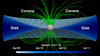 |
Fig. 1. Initial conditions for the reference case. In blue we present in logarithmic scale the density map of the disk, the green lines show the sampled magnetic field lines, and the white sphere represents the stellar surface that marks a boundary. |
2.1. Equations
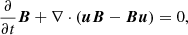
The system is described by solving the time dependent MHD equations in a 3D spherical coordinate system (R, θ, ϕ), including effects of gravitational force from the star, disk viscosity, thermal conduction that also includes the effects of heat flux saturation, coronal heating (using a phenomenological term composed of a steady-state component and a transient component; see Sect. 2.3), and the radiative losses from optically thin plasma. The time-dependent MHD equations are
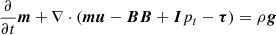
![$$ \begin{aligned}&\frac{\partial }{\partial t}\rho E+\nabla \cdot [(\rho E+p_t){\boldsymbol{u}}-{\boldsymbol{B}}({\boldsymbol{u}}\cdot {\boldsymbol{B}})-{\boldsymbol{u}}\cdot {\boldsymbol{\tau }}] = \nonumber \\&\qquad {\boldsymbol{m}}\cdot {\boldsymbol{g}} - \nabla \cdot F_c - n_e n_H {\Lambda }(T) + Q(R, \theta , \phi , t) \end{aligned} $$](/articles/aa/full_html/2019/04/aa34342-18/aa34342-18-eq3.gif)
where
are the total pressure (thermal and magnetic) and the total gas energy per unit mass (thermal, bulk kinetic, and magnetic), ρ is the density, m = ρu is the momentum density, u is the fluid bulk velocity, B is the magnetic field, I the identity matrix, τ is the viscous stress tensor that we treat below in more detail, g = −∇Φg is the gravity acceleration vector, Φg = GM⋆/R is the gravitational potential of a central star of mass M⋆ at a distance R, G is the gravitational constant, Fc is the heat conductive flux, ne and nH are the electron and hydrogen number density, Λ(T) is the optically thin radiative losses per unit emission measure, T is the fluid temperature, and Q(R, θ, ϕ, t) is a function of space and time describing the phenomenological heating rate (see Sect. 2.3). We used the ideal gas law P = (γ − 1)ρϵ, where γ is the adiabatic index and ϵ is the thermal energy density. The radiative losses were defined for T > 104 K and were derived with the PINTofALE (Kashyap & Drake 2000) spectral code and with the APED v1.3 atomic line database assuming metal abundances equal to 0.5 of the solar value (Anders & Grevesse 1989).
We assumed the viscosity to be effective only in the circumstellar disk and negligible in the extended stellar corona. The transition between corona and disk was outlined through a passive tracer (Cdisk) that is passively advected in the same manner as density (see Paper I for more details). The tracer was initialized with Cdisk = 1 in the disk region and Cdisk = 0 elsewhere. During the system evolution, the disk material and the corona mixed, leading to regions with 0 < Cdisk < 1. The viscosity works only in regions with Cdisk > 0.99, that is, in zones consisting of more than 99% of disk material. The viscous tensor is defined as
![$$ \begin{aligned} \tau = \eta _v \left[(\nabla {\boldsymbol{u}} ) + (\nabla {\boldsymbol{u}})^T -\frac{2}{3}(\nabla \cdot {\boldsymbol{u}}){\boldsymbol{I}} \right], \end{aligned} $$](/articles/aa/full_html/2019/04/aa34342-18/aa34342-18-eq6.gif)
where ηv = νvρ is the dynamic viscosity, and νv is the kinematic viscosity. The accepted scenario considers the turbulence in the disk as the main responsible factor for the losses of angular momentum (Shakura & Sunyaev 1973), possibly triggered by MRI (Balbus & Hawley 1991, 1998). Because it is difficult to describe the phenomenon and we know little about its details, the efficiency of angular momentum transport within the disk is in general described through a phenomenological viscous term that is modulated through the Shakura–Sunyaev α-parameter (e.g., Romanova et al. 2002, Paper I). As in Paper I, the kinematic viscosity was expressed as  is the isothermal sound speed, ΩK is the Keplerian angular velocity, and α < 1 is a dimensionless parameter regulating the efficiency of angular momentum transport within the disk. Simulations of Keplerian disks indicate that the turbulence-enhanced stress tensor, which is responsible for the outward transport of energy and angular momentum, has a typical dimensionless value ranging between 10−3 and 0.6 (Balbus 2003). In our simulations, we assumed α = 0.02 (according to Romanova et al. 2002).
The thermal conduction is anisotropic because of the stellar magnetic field, and it is highly reduced in the direction transverse to the magnetic field. We split the thermal conduction into two components, one along and the other across the magnetic field lines, Fc = F∥i + F⊥j. To allow for a smooth transition between the classical and saturated conduction regimes, we followed Dalton & Balbus (1993) and described the two components of thermal flux as (see also Orlando et al. 2008)
![$$ \begin{aligned}&F_{\parallel } = \left(\frac{1}{\left[q_{\rm spi}\right]_{\parallel }} +\frac{1}{\left[q_{\rm sat}\right]_{\parallel }} \right)^{-1} \end{aligned} $$](/articles/aa/full_html/2019/04/aa34342-18/aa34342-18-eq8.gif)
![$$ \begin{aligned}&F_{\perp } = \left(\frac{1}{\left[q_{\rm spi}\right]_{\perp }} +\frac{1}{\left[q_{\rm sat}\right]_{\perp }} \right)^{-1,} \end{aligned} $$](/articles/aa/full_html/2019/04/aa34342-18/aa34342-18-eq9.gif)
where [qspi]∥ and [qspi]⊥ are the classical conductive flux along and across the magnetic field lines, respectively, according to Spitzer (1962), that is,
![$$ \begin{aligned}&\left[q_{\rm spi}\right]_{\parallel } = -k_{\parallel }\left[\nabla T\right]_{\parallel } = -9.2\times 10^{-7} T^{5/2} \left[\nabla T\right]_{\parallel } \end{aligned} $$](/articles/aa/full_html/2019/04/aa34342-18/aa34342-18-eq10.gif)
![$$ \begin{aligned}&\left[q_{\rm spi}\right]_{\perp } = -k_{\perp }\left[\nabla T\right]_{\perp } = -3.3\times 10^{-16}n_H^2/(T^{1/2}B^2)\left[\nabla T\right]_{\perp ,} \end{aligned} $$](/articles/aa/full_html/2019/04/aa34342-18/aa34342-18-eq11.gif)
where k∥ and k⊥ are both in units of erg K−1 s−1 cm−1 and [∇T]∥ and [∇T]⊥ are the thermal gradients along and across the magnetic field lines. If the spatial scale of the characteristic change in temperature becomes too short compared to the electron mean-free path, the heat flux saturates and the conductive flux along and across the magnetic field lines can be described as (Cowie & McKee 1977)
![$$ \begin{aligned}&\left[q_{\rm sat}\right]_{\parallel } = -\mathrm {sign}(\left[\nabla T\right]_{\parallel }) 5 \phi \rho c_s^3 \end{aligned} $$](/articles/aa/full_html/2019/04/aa34342-18/aa34342-18-eq12.gif)
![$$ \begin{aligned}&\left[q_{\rm sat}\right]_{\perp } = -\mathrm {sign}(\left[\nabla T\right]_{\perp }) 5 \phi \rho c_{\rm s}^3, \end{aligned} $$](/articles/aa/full_html/2019/04/aa34342-18/aa34342-18-eq13.gif)
where cs is the isothermal sound speed, and ϕ, called flux limit factor, is a free parameter between 0 and 1 (Giuliani 1984). For this work, ϕ = 1 as suggested for stellar coronae (Borkowski et al. 1989; Fadeyev et al. 2002).
The calculations were performed using PLUTO, a modular Godunov-type code for astrophysical plasmas (Mignone et al. 2007). The code is designed to use parallel computers using Message Passage Interface (MPI) libraries. The MHD equations were solved using the MHD module available in PLUTO with the Harten-Lax-van Leer Riemann solver. The time evolution was solved using a second-order Runge-Kutta method. The evolution of the magnetic field was calculated using the constrained transport method (Balsara & Spicer 1999), which maintains the solenoidal condition at machine accuracy. We adopted the “magnetic field-splitting” technique (Tanaka 1994; Powell et al. 1999; Zanni & Ferreira 2009) by splitting the total magnetic field into a contribution from the background stellar magnetic field and a deviation from this initial field; then, only the latter component was computed numerically. Radiative losses Λ were calculated at the temperature of interest using a lookup table and interpolation method. Thermal conduction was treated with a super-time-stepping technique, the superstep consists of a certain number of substeps that are properly chosen for optimization and stability, depending on the diffusion coefficient, grid size, and free parameter ν < 1 (Alexiades et al. 1996). The viscosity was solved with an explicit scheme, using a second-order finite difference approximation for the dissipative fluxes.
2.2. Initial and boundary conditions
As in Paper I, we adopted the initial conditions introduced by Romanova et al. (2002), describing the star–disk system in quiescent configuration. In particular, the initial corona and disk were set in order to satisfy mechanical equilibrium among centrifugal, gravitational, and pressure gradient forces (see Paper I and Romanova et al. 2002 for more details); all the plasma is barotropic and the disk and the corona are both isothermal with temperatures Td and Tc, respectively. The stellar rotation axis was set normal to the disk mid-plane, and the protostar was characterized by a rotational period of 9.2 d (see Paper I). The isothermal disk was at Td = 104 K and dense (see Table 1); the disk rotated with Keplerian velocity about a rotational axis aligned with the magnetic dipole. In the initial condition the disk was truncated at the radius Rd, where the ram pressure of the disk plasma is equal to the magnetic pressure. In our setup the corotation radius (where the disk rotates with the same angular velocity of the protostar) was Rco = 8.6 R⋆ (see Paper I). The corona was initially isothermal with temperature Tc = 4 MK (see Paper I).
Model parameters defining the initial conditions of the 3D simulations.
We simulated one half of the whole spatial domain in spherical geometry. Thus, the computational domain extends between Rmin = R⋆ and Rmax = 14 R⋆ in the radial coordinates, between θmin = 5° and θmax = 174° in the angular coordinate θ and between ϕmin = 0 and ϕmax = 180° in the angular coordinate ϕ. The inner and outer θ boundaries do not correspond to the rotational axis to avoid very small δϕ that increase the computational cost and add no significant insight (see Paper I for more details). The radial coordinate was discretized using a logarithmic grid with 128 points with the mesh size increasing with R, to achieve a high resolution close to the stellar surface ΔRmin ≈ 3 × 109 cm and a low resolution in the outer part ΔRmax ≈ 4 × 1010 cm. The θ and ϕ coordinates grids were uniformly sampled and composed of 128 points each, corresponding to the resolution of Δθ ≈ 1.3° and Δϕ ≈ 1.4°, respectively
Our choice to consider only one half of the whole spatial domain was aimed at reducing the computational cost due to the complex dynamics of flares, which requires including radiative cooling and thermal conduction. The main consequence of this choice is that it introduces a long-wavelength cutoff on the perturbation spectrum of the disk. For instance, long-wavelength modes participating in the development of instability at the disk truncation radius are not represented in our model. Nevertheless, we expect that these particular perturbations are not likely to dominate the system evolution; morerover, the study of these perturbations is beyond the scope of this study.
The radial internal boundary condition was defined assuming that the infalling material passes through the surface of the star as in Romanova et al. (2002), thus ignoring the dynamic of the plasma after it impacts onto the stellar surface. A zero-gradient boundary condition was set at Rmax and at the boundaries of θmin and θmax. Periodic boundary conditions were set at ϕmin and ϕmax.
2.3. Coronal heating and flaring activity
The term Q(R, θ, ϕ, t) in Eq. (3) is a phenomenological heating function. It is prescribed as a stationary component, plus a transient component in analogy with the function proposed by Barbera et al. (2017). The former was chosen to exactly balance the radiative losses below 1 MK in the corona, and maintained an initial quasi-stationary extended tenuous corona.
The transient component describes a storm of low to intermediate flares that occur in proximity of the disk. This component is expected to mimic the flaring activity that may be driven by a stressed field configuration resulting from the twisting of magnetic field lines induced by the differential rotation of the inner rim of the disk and the stellar photosphere (Shu et al. 1997).
Each flare was triggered by injecting a localized release of energy that produces a heat pulse. All the pulses had a 3D Gaussian spatial distribution with a width of σ = 2 × 1010 cm. The pulses were randomly distributed in space close to the disk surface at radial distances between the truncation radius and the corotation radius. The flares had a randomly generated timing in order to achieve an average frequency of flare per hour of either one or four flares. The total energy released in a single pulse was also randomized, and it ranged in particular between 1032 and 1034 erg. The total time duration of each pulse was 300 s, then the pulse was switched off. The short duration of the pulses was chosen to describe an impulsive release of energy. Tests performed in Paper I proved that a duration of 300 s represents the minimum pulse duration that can be managed by the code. The time evolution of pulse intensity consists of three equally spaced phases of 100 s each: a linearly increasing ramp, a steady part, and a linearly decreasing ramp.
3. Results
Our model solutions depend on a number of physical parameters, among which the most notable are the density of the disk and the frequency of flares. In the light of this, we considered as a reference case (run FL-REF in Table 1) the disk configuration investigated in Paper I, which is characterized by a maximum density in the equatorial plane of 2.34 × 1010 cm−3 and a frequency of flares of four per hour. Then we explored the case of a disk that was five times denser than in the reference case (run FL-HD), and the case of a frequency of flares four times lower than in the reference case (run FL-LF). We also considered an additional simulation identical to the run FL-HD, but without flares (run NF), to highlight the role played by the flares in the formation of accretion columns in the timescales we covered. We considered the case with the densest disk because we expect a more efficient interaction between disk and stellar magnetosphere, which helps the formation of accretion columns. The simulation FL-HD generates the highest accretion rates (≈10−9 M⊙ yr−1; see Fig. 8). Table 1 summarizes the various simulations and the main parameters that are characteristic of each run: ρd is the maximum density of the disk in the equatorial plane, ρc is the density of the corona close to the disk, and Ffl is the flare frequency.
Our main focus here is on exploring the role played by the flares in perturbing the accretion disk and possibly in triggering accretion on timescales shorter than those if flares were not present. For this reason, we stopped the simulations when the accretion rates reached a quasi-stationary regime after the initial sudden and steep rise (see Sect. 3.3); our simulations cover about three days of evolution (≈1/3 of the rotational period of the inner disk).
We followed the evolution of the system without flares (i.e., run NF) for about four days (i.e., on a timescale larger than that covered by the other simulations). We note that the initial conditions adopted provide quasi-equilibrium. The disk was initially truncated at 2.86 R⋆. When the simulation started, the magnetic field lines of the slowly rotating magnetosphere threading the disk exerted a torque on the faster-rotating disk. As a result, the inner part of the disk moved inward on a timescale that was shorter than the viscous timescale, and matter gradually accumulated in proximity of the truncation radius located at Rd ≈ 2.1 R⋆ at the end of the simulation. As shown by long-term 3D simulations (e.g., Romanova et al. 2002, 2011a; Kulkarni & Romanova 2008), this process of inward motion of matter at some point leads to accretion onto the star without any need of flares. However, run NF shows that this initial torque helps to bring matter toward the magnetosphere of the star, but no accretion stream develops in the timescale we considered. By the end of the simulation, there is a hint of mass accretion that leads to rates on the order of 10−10 M⊙ yr−1 (about an order of magnitude lower than in the corresponding simulation with flares; see Fig. 8). We conclude that higher levels of accretion driven by the magnetic torque in our star-disk system start on timescales longer than about four days. In the following, we discuss in detail the simulations, including the effect of flares. In the light of the results of run NF, we are confident that disk perturbations and the accretion rates found in the timescale we considered are entirely due to the flaring activity.
3.1. Reference case
For the reference case FL-REF, we followed the evolution of the flaring activity on the star-disk system for approximately three days (i.e., when a stationary regime was reached). Figure 2 shows representative frames to describe this evolution. A movie showing the entire evolution is provided as online material (Movie 1). The movie shows the evolution of FL-REF. Each frame is composed of three panels: at the top, an edge-on view of the system, at the bottom left and right, the two pole-on views. The movie shows the mass density (blue) and sampled magnetic field lines (green). A 3D volume rendering of the plasma temperature is overplotted in log scale and shows the flaring loops (red-yellow).
 |
Fig. 2. Evolution of the reference case FL-REF. Each of the six panels shows a snapshot at a given time after the initial condition (defined in Sect. 2 in Fig. 1) at 1.17 h (panel A), 3.51 h (panel B), 15.08 h (panel C), 23.4 h (panel D), 30.55 h (panel E), and 48.88 h (panel F). Each panel is composed of three images: at the top, an edge-on view of the 3D system, at bottom left and right, the two pole on views. The cutaway views of the star-disk system show the mass density (blue) and sampled magnetic field lines (green) at different times. A 3D volume rendering of the plasma temperature is overplotted in log scale on each image and shows the flaring loops (red-yellow) that link the inner part of the disk with the central protostar. The color-coded density logarithmic scale is shown on the left of each panel, and the analogously coded temperature scale is on the right. The white arrows indicate the rotational direction of the system. The physical time since the start of the evolution is shown at the top center of each panel. |
As discussed in Sect. 2.3, the heat pulses triggering the flares are injected into the system at randomly chosen locations above and below the disk through the phenomenological term Q(R, θ, ϕ, t) in Eq. (3). We found that the evolution of each flare is analogous to the evolution of the single bright flare analyzed in Paper I. For example, this is evident for the first flare in run FL-REF, which occurs after about one hour since the initial condition (see the lower right panel in Fig. 2 A-B and Movie 1) and is not perturbed by other flares during its entire lifetime.
The initial heat pulse determines a local increase in plasma pressure and temperature close to the disk surface. As a result, the disk material is heated up and rapidly expands through the overlying hot and tenuous corona, resulting in a strong evaporation front. The disk evaporation is sustained by thermal conduction from the outer layers of hot plasma even after the heat pulse ends. The fraction of this hot expanding material closer to the protostar is confined by the magnetic field due to β < 1 and forms a hot (temperature of about 107 − 109 K) magnetic loop with a length on the order of 1011 cm that links the disk to the stellar surface. The magnetic-field-oriented thermal conduction furthers the development of this hot loop through the formation of a fast thermal front propagating from the disk along the magnetic field lines toward the star. The remaining part of the evaporating plasma that is not channeled in the loop is poorly confined by the magnetic field (due to β > 1). Thus it moves away from the system toward regions with higher β, carrying away mass and angular momentum from the system (see below). In any case, the plasma (either magnetically confined or non-confined) starts to cool down as soon as the heat deposition ends because of the combined action of radiative losses, thermal conduction, and plasma expansion. After about 10 h, the hot loop disappears.
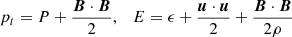
Figure 3 shows the evolution of the maximum temperature and emission measure (EM) of the second flaring loop (see Fig. 2 B and Movie 1). This evolution can be considered to be representative of all the flares simulated here and is analogous to that observed on Sun and stars. We distinguished two different phases in the evolution: a heating and a cooling phase. The first starts with the injection of the heat pulse and lasts for a few hundred seconds. During this phase the temperature increases very rapidly and reaches maximum at ≈109 K. The disk material evaporates under the effect of the thermal conduction and the heated plasma expands, filling a magnetic flux tube that links the disk with the star. As a result, the EM rapidly increases and peaks at later times, about 6 min after the maximum temperature. At later times, the radiative losses and the thermal conduction very efficiently cool the plasma down and the cooling phase starts. Both the temperature and the EM decrease slowly. After about four hours since the heating, the temperature of the flaring plasma is still on the order of 107 K. The EM develops a second bump about one hour after the peak, which is at odds with the expected evolution on the base of 1D models of flares (e.g., Reale et al. 1988). As discussed in Paper I, each flare of our simulations is only partially confined by the magnetic field at the loop footpoint anchored at the disk surface, which is at variance with 1D models where the flares are assumed to be fully confined by the magnetic field. The second bump of EM in Fig. 3 originates from the fast expansion of the non-confined hot plasma in the surrounding environment. From this point of view, our simulated flares can be considered to be intermediate between those of models of fully confined flares (e.g., Reale et al. 1988) and those of models of non-confined flares (e.g., Reale et al. 2002). We also note that the magnetic field in the domain is idealized. In a more realistic case the evolved magnetic field may have a more complex configuration, and may be more intense than in the case studied because of magnetic field twisting. For this reason we expect to observe a greater confinement in a real case than in the simulations.
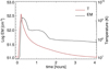 |
Fig. 3. Evolution of the maximum temperature (red line) and integrated EM (black line) of the plasma with log(T) > 6.3 for the second flare in run FL-REF. The initial time is at the release of the corresponding heat pulse. |
In addition to the formation of the hot loop, the initial heat pulse produces an overpressure wave at the loop footpoint that is anchored to the disk, which propagates through the disk. In the case of the energetic flare investigated in Paper I, when the overpressure reaches the opposite side of the disk, it pushes the material out of the equilibrium position and drives it into a funnel flow (see Paper I for more details). Then the gravitational force accelerates the plasma toward the central star where the accretion stream impacts. In run FL-REF, however, the flares are less energetic than the flare in Paper I. The overpressure wave generated by the first flare is not strong enough to significantly perturb the disk and to eventually trigger an accretion event.
After the first flare, other flares occur close to the disk surface. Each of them produces a significant amount of hot plasma (with temperatures up to ≈109 K) that is thrown out in the magnetosphere (Fig. 2 C–F and Movie 1). As for the first flare, part of this hot material is channeled by the magnetic field in flux tubes that form hot magnetic loops that link the disk to the central protostar. Nevertheless, most of the evaporated disk material is poorly confined by the magnetic field (especially in flares that occur at larger distances from the star) and it escapes from the system, contributing to the plasma outflow from the star with a mass loss rate Mloss ≈ 10−10 M⊙ yr−1 and angular momentum loss rate Lloss ≈ 106 − 107 g cm yr−1. As a result, the magnetic field lines are gradually distorted by the escaping plasma. All this hot plasma, either confined to loops or escaping from the star, forms an extended hot corona that once formed, persists until the end of the simulation.
Figure 4 shows the evolution of the integrated EM of the whole system. After the first heat pulse, the emission measure increases rapidly. In this transient phase, the extended corona is not developed yet and the effect of each heat pulse is clearly visible in the curve with the sudden increase and slower decay of EM. After the first flares, the amount of plasma at temperatures greater than 2 MK continues to increase, reaching a quasi-stationary regime after ≈10 h. At this time the hot extended corona is well developed. The resulting values of EM for plasma above 2 MK indicate that the flaring activity is expected to produce a significant X-ray emission. During this phase, the pronounced peaks of EM are produced by the most energetic flares.
 |
Fig. 4. Evolution of the integrated EM for plasma with log(T) > 6.3 for the run FL-REF. The red square is zoomed-in in Fig. 3. |
We synthesized the X-ray luminosity (LX) in the band [1,10] keV from the reference case. We applied a procedure analogous to the one described in Paper I (see also Barbera et al. 2017). We found that during the stationary phase, LX ≈ 1030erg s−1. This value is in the range of luminosities typically inferred from observations (Preibisch et al. 2005). A detailed study of the evolution and origin of the X-ray emission will be the subject of a future paper.
As for the first flare, each subsequent abrupt release of energy produced a local increase in plasma pressure in regions of the disk that correspond to the loop footpoints. These local increases in pressure produce overpressure waves that propagate through the disk. In general, given the low energy of most of the flares, the single overpressure wave is not sufficient to significantly perturb the disk and trigger an accretion column. However, the combination of a series of these overpressures can strongly perturb and distort the disk, especially in proximity of the truncation radius (see Fig. 2 F and Movie 1). Eventually, the overpressures can produce mass accretion episodes. After ≈15 h, several accretion columns start to develop (Fig. 2 C and Movie 1). The first column impacts onto the stellar surface after ≈23 h (Fig. 2 D and Movie 1). Then, the accretion process continues until the end of the simulation.
The dynamics of the accretion columns is complex, as expected because the corotation radius of our system (Rco = 8.6R⋆) is much larger than the magnetospheric radius (≈2 − 3 R⋆). In these conditions, the material accretes in a strongly unstable regime (Blinova et al. 2016), where one or two unstable filaments (“tongues”) form and rotate approximately with the angular velocity of the inner disk. In our simulation, the system evolution is analogous and accretion columns develop from the disk surface in regions close to the truncation radius. There, the disk material is channelled by the magnetic field in accretion streams that accelerate toward the central star under the effect of gravity. Then the accretion streams impact onto the stellar surface at high latitudes (> 40°; see Sect. 3.4). The accretion pattern suggests accretion driven by Rayleigh–Taylor (RT) instability (e.g., Blinova et al. 2016). As expected for RT unstable accretion, the formation of small-scale filaments along the edge of the disk and the formation of several funnels is indeed visible. Their occurrence and shape are typical of unstable tongues: they form frequently and disappear rapidly, and they are initially tall and narrow (e.g., Kulkarni & Romanova 2008, 2009; Romanova et al. 2008; Blinova et al. 2016). In 3D simulations of accretion onto stars with a tilted dipole, the instability is triggered and supported by the non-axisymmetry introduced by the dipole and by the pressure gradient force that develops close to the truncation radius through accumulation of matter by disk viscosity (Romanova et al. 2012). In our case of a non-tilted dipole-octupole simulated on short timescales, the X-ray flares provide the necessary amount of non-axisymmetry and determines the pressure gradient force to start and support accretion through instability. In the simulation without flares (run NF), no sign of instability is present in the timescale covered (about four days). Therefore, even if matter were to accrete onto the protostar through MHD processes of the disk-magnetosphere interaction, this phenomenon would occur on timescales longer than those covered here in our simulations. The flares therefore provide the conditions to speed up the process on timescales significantly shorter (only a few hours) than those present in the case without flares.
The streams can be heavily perturbed during their lifetime by the flaring activity and by other streams. For instance, a flare occurring on the opposite side of the disk may trigger an overpressure wave that may enhance the accretion rate of the stream. A flare occurring close to the accretion column may inject more mass into the stream increasing its lifetime (see Fig. 5) or it may produce a perturbation that is strong enough to disrupt the base of the stream and, as a consequence, the whole accretion column. The streams may interact with each other, merging into larger streams (see Movie 1). As a result of this complex dynamic, the streams are highly unstable and time variable, and the accretion columns are highly inhomogeneous, structured in density, and clumped (e.g., Matsakos et al. 2013; Colombo et al. 2016). This may support the idea that the persistent low-level hour-timescale variability observed in CTTSs may reflect the internal clumpiness of the streams (Gullbring et al. 1996; Safier 1998; Bouvier et al. 2007b; Giardino et al. 2007; Cranmer 2009).
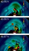 |
Fig. 5. Example of the perturbation of an accretion column by nearby flaring activity. The figure shows snapshots displaying isosurfaces where the particle number density equals 5 × 109 cm−3 in run FL-REF. We show the southern pole-on view of the star. The isosurfaces, which coincide with the cold and dense disk material, are shown at the labeled times (upper left corner of each panel). The colors give the pressure (in units of dyn cm−2) on the isosurface, and the color-coding is defined on the right of each panel. Upper panel: red arrow points at flare that perturbs the accretion column (see high-pressure region in the disk). Middle and lower panel: red arrow points at the portion of the disk material that perturbs the accretion column. |
3.2. Comparison with other models
We explored the effects of either the disk density or the flare frequency on the dynamics of the star-disk system. To this end, we considered the case of a disk that was five times denser than in the reference case (run FL-HD in Table 1) and had the same sequence of flares. We found that the evolution in run FL-HD is analogous to that of the reference case. In particular, the random heat pulses produce hot plasma in proximity of the disk surface; then part of this plasma is channeled in hot loops, and the other part escapes from the system. All this hot material forms an extended and structured hot corona. As for the reference case, the heat pulses also generate overpressure waves that propagate through the disk, eventually pushing the disk material out of equilibrium to form accretion columns. In the case of a denser disk, however, the effects of these waves moving through the disk are mild in comparison with run FL-REF. The perturbation of the disk is limited to the surface of the disk and the latter is less distorted than in FL-REF (see Figs. 6–7). Nevertheless, the disk material channeled in accretion streams is on average denser than in FL-REF so that the accretion columns are in general denser than in the reference case (see Fig. 6).
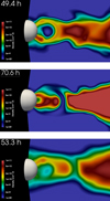 |
Fig. 6. Close-up view of the structure of the accretion columns for runs FL-REF (top panel), FL-HD (middle panel), and FL-LF (bottom panel). Each panel shows a slice in the (R, z) plane passing through the middle of one of the streams. The white hemisphere represents the stellar surface. |
For the dependence of the system evolution on the flare frequency, we found that the dynamics can be significantly different if the flare frequency is four times lower than in FL-REF. In this case, the system needs more time for a significant perturbation of the disk that is able to produce mass accretion onto the central protostar. The dynamics of the accretion columns, once formed, is similar to that in runs FL-REF and FL-HD. The main difference is the number of streams, which is lower in run FL-LF than in the other two cases. This is a direct consequence of the lower number of flares in run FL-LF, which can contribute to the disk perturbation with their overpressure waves. After about 60 h, only one prominent accretion column is present, whereas in runs FL-REF and FL-HD, two or more accretion columns are clearly visible (see Fig. 7). Nevertheless, a significant mass accretion is present in the system at the end of the simulation, even though the flare frequency is lower than in FL-REF.
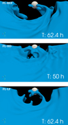 |
Fig. 7. Representative close up views of the inner region of the star-disk system for runs FL-REF (top panel), FL-HD (middle panel), and FL-LF (bottom panel). In blue we show the isosurfaces where the disk material has a particle number density n = 1010 cm−3. The white sphere in each panel represents the stellar surface. |
3.3. Accretion rates
From the modeling results, we derived the mass accretion rates due to the various streams triggered by the flares. We considered as accreting material the amount of mass that crosses the internal boundary representing the stellar surface, namely the material that falls onto the central star. Figure 8 shows the evolution of the accretion rates for the four simulations in Table 1. The three cases with flares show qualitatively the same trend. After the first stream hits the stellar surface (during the first 20 h of evolution; in run FL-LF this occurs after about 50 h), the accretion rate rapidly increases due to the rapid development of new accretion columns. This phase is transient and lasts for about 10 h (see Fig. 2 D and Movie 1). After this, the accretion rate increases more slowly and enters a phase in which the number of active accretion columns is roughly constant.
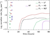 |
Fig. 8. Evolution of accretion rates synthesized from runs FL-RF (black line), FL-HD (red line), FL-LF (green line), and NF (purple line). The crosses represent the values of mass accretion rates inferred from optical-near UV observations for a sample of low-mass stars and brown dwarfs (green, Herczeg & Hillenbrand 2008), for a sample of solar-mass young accretors (red, Herczeg & Hillenbrand 2008), and for an X-ray-selected sample of CTTSs (blue, Curran et al. 2011); their position on the time axis is chosen to facilitate comparison with the model results. |
After the transient phase, the three cases show accretion rates ranging between ≈10−10 M⊙ yr−1 and ≈10−9 M⊙ yr−1, with the highest values shown by run FL-HD because the streams are denser than in the other two cases, and FL-LF and FL-REF show the lowest values because the disk is less dense (see Sect. 3.2). After about 70 h of evolution, run FL-LF shows accretion rates that are comparable to those of run FL-REF. These two cases differ only for the frequency of flares, and they consider the same density structure of the disk; thus run FL-LF needs more time to reach the accretion rate values shown in run FL-REF. We conclude that the accretion rates depend more strongly on the disk density than on the flare frequency.
The simulation without flares (run NF) does not show accretion during the first approximately 65 h of evolution. In this time the magnetic torque brings matter toward the magnetosphere of the star, and after 65 h leads to inflow of matter that generates a sudden increase in the accretion rate up to ≈10−10 M⊙ yr−1. The rate then slowly increases until the end of the simulation, when it reaches values that do not exceed ≈3 × 10⁻¹⁰ M⊙ yr−1. In the corresponding simulation with flares (run FL-HD), the accretion starts much earlier, about 20 hours after the start of the simulation, with rates more than an order of magnitude higher than in run NF on the timescale we covered. The disk perturbation and the mass accretion we observed in simulations with flares are therefore due to the flaring activity in proximity of the disk.
We compared the accretion rates derived from our 3D simulations with those available in the literature derived from optical–UV observations. In particular, we considered two samples of low-mass young accreting stars analyzed by Herczeg & Hillenbrand (2008) that were observed with the Low Resolution Imaging Spectrometer (LRIS) on Keck I and with the Space Telescope Imaging Spectrograph (STIS) on board the Hubble Space Telescope, and an X-ray selected sample of CTTSs analyzed by Curran et al. (2011) that was observed with various optical telescopes. We found that the three simulations reproduce most of the accretion rates measured in low-mass stars quite well and are lower than those of fast-accreting objects such as BP Tau, RU Lup, or T Tau. On the other hand, it is worth noting that the timescale we explored here is rather short (about 80 h) so that the disk viscosity, for instance, has a negligible effect on the dynamics.
3.4. Hotspots
The disk material flowing through the accretion columns is expected to impact onto the stellar surface and to produce shock-heated spots. We do not have enough spatial resolution in our simulations to model these impacts (see, e.g., Orlando et al. 2010, 2013). The model does not include a description of the chromosphere of the CTTS either, which would be necessary to produce shocks at the base of accretion columns after the impacts. Nevertheless, we can infer the expected size and evolution of the hotspots and the latitudes where the spots are located from the simulations.
Figure 9 shows maps of particle number density close to the stellar surface after about 60 h of evolution (when the accretion columns are well developed). A movie showing the time evolution of particle number density on the stellar surface is available as online material (Movie 2). The movie shows the evolution for FL-REF of the particle number density in log scale close to the stellar surface. During the initial transient phase, only a few (one or two) small and faint hotspots are present on the stellar surface, each corresponding to an accretion column (Fig. 2 D–E and Movie 1). At later times, the number of accretion columns in general increase following the disk perturbation that is due to the flares (Fig. 2 F and Movie 1). The number of hotspots, however, does not increase with the number of accretion columns, and no more than four spots are visible on the stellar surface during the whole evolution (see Fig. 9). The accretion streams interact with each other and often merge to form larger accretion columns before impact (Fig. 2 F and Movie 1). This complex dynamics is typical of accretion in the strongly unstable regime, where smaller tongues merge and form one or two larger tongues (e.g., Blinova et al. 2016). As a result, the spots are larger at later times.
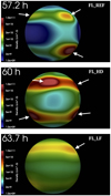 |
Fig. 9. Maps of particle number density in log scale close to the stellar surface after about 60 h of evolution for runs FL-REF (upper panel), FL-HD (middle panel), and FL-LP (lower panel). The high-density regions (pointed at by white arrows) correspond to accretion columns impacting onto the stellar surface. Runs FL-REF and FL-HD exhibit clear hotspots, whereas in run FL-LF, the matter is more diffused and the contrast in density is weaker. |
In the reference case (FL-REF), two prominent hotspots are evident in the visible hemisphere of the star (top panel of Fig. 9) both with a density of around 3 × 1010 cm−3 (the shock-heated plasma after impact is expected to be four times denser in strong-shock conditions; e.g., Sacco et al. 2010). A slightly fainter (density of about 1010 cm−3) spot is also present in the northern hemisphere. The spots cover a significant portion of the stellar surface (≈20%). Simulation FL-HD (middle panel of Fig. 9) shows a similar density structure on the stellar surface. In this case, three large hotspots with a density of between 1010 and 5 × 1010 cm−3 are present in the visible hemisphere of the star. In this case, the filling factor of the spots is ≈30%. Run FL-LF presents a density structure on the stellar surface that is significantly different than in the other two cases. The density contrast of the spots is much weaker than in runs FL-REF and FL-HD. A main hotspot with density ρ ≈ 2 × 1010 cm−3 and two less dense (ρ ≈ 1010 cm−3) and smaller spots are present in the visible hemisphere. In this case, the filling factor of the spots is lower than 10%.
Figure 9 also shows that the hotspots are characterized by a dense inner core that is surrounded by lower density material as found by Romanova et al. (2004; see also Bonito et al. 2014). The spots are clearly visible in runs FL-REF and FL-HD (in general, yielding higher accretion rates); in run FL-LF, the accreted matter is more diffuse throughout the entire stellar surface and the spots have a lower contrast in density. In all the explored cases, the accretion occurs preferentially at high latitudes and the hotspots are located above (below) 40° (−40°); this is an effect of the magnetic field configuration chosen for the model (see Sect. 2 and, e.g., Romanova et al. 2011b). More specifically, high-latitude hotspots are favored when dipole and octupole components are parallel (e.g., Romanova et al. 2011b); conversely, if dipole and octupole components are antiparallel, low-latitude spots are favored (e.g., Donati et al. 2011). Earlier 3D simulations of accretion onto stars with dipole-plus-octupole aligned components (as in our case) have shown that the octupole component dominates in driving matter closer to the star, guiding the flows toward the high-latitude poles, and part of the matter into octupolar belts or rings (e.g., Long et al. 2008, 2011; Romanova et al. 2011a,b). As a result, the shape and position of the hotspots differ from those expected in a pure dipolar case, where the spots are typically observed at intermediate latitudes. In our simulations, we observe that initially, the matter flows into accretion streams guided by the dipole magnetic field. Then, the trajectory of the flows is sligthly redirected in proximity of the star, at distances below ≈1.7 R⋆, by the dominant octupole component.
3.5. Limits of the model
Our setup is analogous to others that have often been used in the literature (e.g., Romanova et al. 2002; Orlando et al. 2011) and is appropriate to describing the stellar-disk system in the context of young accreting stars. Nevertheless, a number of simplifications and assumptions have been made that we discuss in the following.
First, many works (e.g., Gregory et al. 2010; Gregory & Donati 2011) suggested that a stellar magnetic field can have a more complex configuration than we adopted here, namely an aligned octupole-dipole. In addition, in our setup, the initial magnetic field configuration does not account for the twisting and expansion of the field lines driven by the differential rotation of the disk and the different rotation period of the disk with respect to the star. A more complex magnetic field configuration is expected to change the dynamics of accretion streams described here, leading to a possibly more complex pattern of accretion. Moreover, we expect that the flares are generated by phenomena such as magnetic reconnection (see Sect. 1). For this reason, in the region where the magnetic field may generate a heat release, we expect an even more complex configuration than that assumed in our simulations. Then, the magnetic confinement of the hot plasma might be more efficient than in our simulations; this should enhance the effects of flare energy deposition in the system.
The description of the viscosity of the disk is simplified. Simulations of MRI suggests that the disk viscosity can be highly inhomogeneous and depending on time (Balbus 2003). However, the timescale considered here (80 h) is negligible compared to the viscosity timescale (several stellar periods, e.g., Romanova et al. 2002; Zanni & Ferreira 2009), we therefore do not expect to observe any effects considering a more realistic viscosity. Last, the description in terms of geometry and duration of the heat release that generates the single flare is idealized (see Sect. 2.3). We expect that the geometry of the heat release strongly depends on the specific magnetic field configuration at the site where the energy release occurs. Moreover, in realistic conditions we do not expect that each heat release would have the same duration as we have assumed. Nevertheless, we are not interested in a detailed study of the flare evolution here, but only in its consequences in terms of dynamical perturbation of the disk. From this point of view, the flares we simulated produce realistic perturbations.
4. Summary and conclusions
We investigated the effects of an intense flaring activity localized in proximity of the accretion disk of a CTTS. To this end, we adopted the 3D MHD model, presented in Paper I, a magnetized protostar surrounded by a Keplerian accretion disk. The model has been adapted to include a storm of flares with low to intermediate intensity that occurs in proximity of the disk. The model takes into account all the relevant physical processes: stellar gravity, viscosity of the disk, thermal conduction, radiative losses from optically thin plasma, and a parameterized heating function to trigger the flares. We explored cases with different disk densities and different levels of flaring activity. Our results lead to the following conclusions.
-
The coronal activity due to a series of low to intermediate flares that occur in proximity of the disk surface heats the disk material to temperatures of several million degrees. Part of this hot plasma is channeled and flows in magnetic loops that link the inner part of the disk to the central protostar; the remaining part of the heated plasma is poorly confined by the magnetic field (especially in flares that occur at larger distances from the star) and escapes from the system, carrying away mass and angular momentum. The coronal loops generated by the flares have typical lengths on the order of 1011 cm, maximum temperatures ranging between 108 K and 109 K, and a lifetime of about 10 h. These characteristics are similar to those derived from the analysis of luminous X-ray flares observed in young low-mass stars (e.g., Favata et al. 2005). The escaping disk material contributes to increase the plasma outflow from the system with mass-loss rates Mloss = 10−10 and angular momentum loss rate Lloss = 106 − 107 g cm
 yr−1. The disk material, either confined in loops or escaping from the star, forms a tenuous hot corona extending from the central protostar to the inner portion of the disk.
 -
The circumstellar disk is heavily perturbed by the flaring activity. In the aftermath of the flares, disk material evaporates in the outer stellar atmosphere under the effect of the thermal conduction. As previously stated in Paper I, overpressure waves are generated by the heat pulses in the disk at the footpoints of the hot loops that form the corona. The overpressure waves travel through the disk and distort its structure. Eventually, the overpressure waves can reach the side of the disk opposite to where heat pulses were injected. There, the overpressure waves can push the disk material out of equilibrium to form funnel flows that accrete disk material onto the protostar. We found that the effects of the overpressure waves are larger in disks that are less dense and for a higher frequency of flares. This type of accretion process starts about 20 hours after the first heat pulse, which is a timescale much shorter than that required by the disk viscosity to trigger the accretion. The accretion rates derived by the simulations range between 10−10 and 10−9 M⊙ yr−1. We found that the higher the disk density, the higher the accretion rate. The accretion rates are comparable with those inferred from observations of low-mass stars and brown dwarfs and in some solar mass accretors (Herczeg & Hillenbrand 2008; Curran et al. 2011).
-
The accretion columns generated by the flaring activity on the disk have a complex dynamics and a lifetime ranging between a few hours and tens of hours. They can be perturbed by the flaring activity itself; for instance, a flare that occurs close to an accretion column can disrupt it or otherwise increase the amount of downfalling plasma. The streams can also interact with each other if they are sufficiently close, possibly merging into larger streams. As a result of this complex dynamics, the streams are highly inhomogeneous, with a complex density structure, and clumped, with clumps of typical size comparable to the section of the accretion column. In general, they have a dense inner core surrounded by lower density material, as has also been found by Romanova et al. (2004). These findings support the idea that the persistent low-level hour-timescale variability observed in CTTSs reflects the internal clumpiness of the streams (Gullbring et al. 1996; Safier 1998; Bouvier et al. 2007b; Giardino et al. 2007; Cranmer 2009).
Our simulations open a number of interesting questions. The hot plasma generated by the flares produces a hot extended corona that irradiates strong X-rays with a different spatial distribution than in the standard scenario of a corona confined to the stellar surface. A corona above the disk irradiates the disk from above with near normal incidence; the radiation reaches outer regions of the disk that may be shielded from the stellar-emitted X-rays. This may influence the chemical and physical evolution of the disk in a different way, with important consequences, for instance, on the formation of planets. This effect can be even more relevant than that due to X-ray emission from the base of protostellar jets located at larger distances from the disks (hundreds of astronomical units; Bonito et al. 2007). In addition, the irradiation produced by the flares can also increase the ionization level of the disk. As a result, a better coupling between magnetic field and plasma can be realized, which might increase the MRI efficiency.
Movies
Movie 1 (Fig. 2) Access here
Movie 2 (Fig. 9) Access here
Acknowledgments
We thank the referee for their comments that helped us to improve the manuscript. PLUTO is developed at the Turin Astronomical Observatory in collaboration with the Department of Physics of Turin University. We acknowledge the “Accordo Quadro INAF-CINECA (2017)” the CINECA Award HP10B1GLGV and the HPC facility (SCAN) of the INAF – Osservatorio Astronomico di Palermo, for the availability of high performance computing resources and support. This work was supported by the Programme National de Physique Stellaire (PNPS) of CNRS/INSU, co-funded by CEA and CNES. This work has been done within the LABEX Plas@par project, and received financial state aid managed by the Agence Nationale de la Recherche (ANR), as part of the programme “Investissements d’avenir” under the reference ANR-11-IDEX-0004-02. The authors (R. B. and C. A.) acknowledge modest financial contribution from the agreement ASI-INAF n.2017-14.H.O.
References
- Aarnio, A. N., Stassun, K. G., & Matt, S. P. 2010, ApJ, 717, 93 [NASA ADS] [CrossRef] [Google Scholar]
- Alexiades, V., Amiez, G., & Gremaud, P. A. 1996, Commun. Numer. Methods Eng., 12, 31 [CrossRef] [Google Scholar]
- Anders, E., & Grevesse, N. 1989, Geochim. Cosmochim. Acta, 53, 197 [Google Scholar]
- Argiroffi, C., Drake, J. J., Bonito, R., et al. 2017, A&A, 607, A14 [NASA ADS] [CrossRef] [EDP Sciences] [Google Scholar]
- Audard, M., Briggs, K. R., Grosso, N., et al. 2007, A&A, 468, 379 [NASA ADS] [CrossRef] [EDP Sciences] [Google Scholar]
- Balbus, S. A. 2003, ARA&A, 41, 555 [NASA ADS] [CrossRef] [Google Scholar]
- Balbus, S. A., & Hawley, J. F. 1991, ApJ, 376, 214 [NASA ADS] [CrossRef] [Google Scholar]
- Balbus, S. A., & Hawley, J. F. 1998, Rev. Mod. Phys., 70, 1 [Google Scholar]
- Balsara, D. S., & Spicer, D. S. 1999, J. Comput. Phys., 149, 270 [Google Scholar]
- Barbera, E., Orlando, S., & Peres, G. 2017, A&A, 600, A105 [NASA ADS] [CrossRef] [EDP Sciences] [Google Scholar]
- Bertout, C., Basri, G., & Bouvier, J. 1988, ApJ, 330, 350 [NASA ADS] [CrossRef] [Google Scholar]
- Bessolaz, N., Zanni, C., Ferreira, J., Keppens, R., & Bouvier, J. 2008, A&A, 478, 155 [NASA ADS] [CrossRef] [EDP Sciences] [Google Scholar]
- Blinova, A. A., Romanova, M. M., & Lovelace, R. V. E. 2016, MNRAS, 459, 2354 [NASA ADS] [CrossRef] [Google Scholar]
- Bonito, R., Orlando, S., Peres, G., Favata, F., & Rosner, R. 2007, A&A, 462, 645 [NASA ADS] [CrossRef] [EDP Sciences] [Google Scholar]
- Bonito, R., Orlando, S., Argiroffi, C., et al. 2014, ApJ, 795, L34 [Google Scholar]
- Borkowski, K. J., Shull, J. M., & McKee, C. F. 1989, ApJ, 336, 979 [NASA ADS] [CrossRef] [Google Scholar]
- Bouvier, J., Alencar, S. H. P., Harries, T. J., Johns-Krull, C. M., & Romanova, M. M. 2007a, Protostars and Planets V, 479 [Google Scholar]
- Bouvier, J., Alencar, S. H. P., Boutelier, T., et al. 2007b, A&A, 463, 1017 [NASA ADS] [CrossRef] [EDP Sciences] [Google Scholar]
- Brickhouse, N. S., Cranmer, S. R., Dupree, A. K., Luna, G. J. M., & Wolk, S. 2010, ApJ, 710, 1835 [NASA ADS] [CrossRef] [Google Scholar]
- Colombo, S., Orlando, S., Peres, G., Argiroffi, C., & Reale, F. 2016, A&A, 594, A93 [NASA ADS] [CrossRef] [EDP Sciences] [Google Scholar]
- Cowie, L. L., & McKee, C. F. 1977, ApJ, 211, 135 [NASA ADS] [CrossRef] [Google Scholar]
- Cranmer, S. R. 2009, ApJ, 706, 824 [NASA ADS] [CrossRef] [Google Scholar]
- Curran, R. L., Argiroffi, C., Sacco, G. G., et al. 2011, A&A, 526, A104 [NASA ADS] [CrossRef] [EDP Sciences] [Google Scholar]
- Dalton, W. W., & Balbus, S. A. 1993, ApJ, 404, 625 [NASA ADS] [CrossRef] [Google Scholar]
- Donati, J.-F., Jardine, M. M., Gregory, S. G., et al. 2007, MNRAS, 380, 1297 [NASA ADS] [CrossRef] [Google Scholar]
- Donati, J.-F., Gregory, S. G., Montmerle, T., et al. 2011, MNRAS, 417, 1747 [NASA ADS] [CrossRef] [Google Scholar]
- Drake, J. J., Ercolano, B., Flaccomio, E., & Micela, G. 2009, ApJ, 699, L35 [NASA ADS] [CrossRef] [Google Scholar]
- Fadeyev, Y. A., Le Coroller, H., & Gillet, D. 2002, A&A, 392, 735 [NASA ADS] [CrossRef] [EDP Sciences] [Google Scholar]
- Favata, F., Flaccomio, E., Reale, F., et al. 2005, ApJS, 160, 469 [NASA ADS] [CrossRef] [Google Scholar]
- Feigelson, E. D., & Montmerle, T. 1999, ARA&A, 37, 363 [NASA ADS] [CrossRef] [Google Scholar]
- Flaccomio, E., Micela, G., & Sciortino, S. 2003a, A&A, 397, 611 [NASA ADS] [CrossRef] [EDP Sciences] [Google Scholar]
- Flaccomio, E., Micela, G., & Sciortino, S. 2003b, A&A, 402, 277 [NASA ADS] [CrossRef] [EDP Sciences] [Google Scholar]
- Getman, K. V., Feigelson, E. D., Grosso, N., et al. 2005, ApJS, 160, 353 [NASA ADS] [CrossRef] [Google Scholar]
- Getman, K. V., Feigelson, E. D., Broos, P. S., Micela, G., & Garmire, G. P. 2008a, ApJ, 688, 418 [NASA ADS] [CrossRef] [Google Scholar]
- Getman, K. V., Feigelson, E. D., Micela, G., et al. 2008b, ApJ, 688, 437 [NASA ADS] [CrossRef] [Google Scholar]
- Giardino, G., Favata, F., Pillitteri, I., et al. 2007, A&A, 475, 891 [NASA ADS] [CrossRef] [EDP Sciences] [Google Scholar]
- Giuliani, Jr., J. L. 1984, ApJ, 277, 605 [NASA ADS] [CrossRef] [Google Scholar]
- Goodson, A. P., & Winglee, R. M. 1999, ApJ, 524, 159 [NASA ADS] [CrossRef] [Google Scholar]
- Goodson, A. P., Winglee, R. M., & Böhm, K.-H. 1997, ApJ, 489, 199 [NASA ADS] [CrossRef] [Google Scholar]
- Gregory, S. G., & Donati, J.-F. 2011, Astron. Nachr., 332, 1027 [NASA ADS] [CrossRef] [Google Scholar]
- Gregory, S. G., Wood, K., & Jardine, M. 2007, MNRAS, 379, L35 [NASA ADS] [CrossRef] [Google Scholar]
- Gregory, S. G., Jardine, M., Gray, C. G., & Donati, J.-F. 2010, Rep. Prog. Phys., 73, 126901 [Google Scholar]
- Gullbring, E., Barwig, H., Chen, P. S., Gahm, G. F., & Bao, M. X. 1996, A&A, 307, 791 [NASA ADS] [Google Scholar]
- Herczeg, G. J., & Hillenbrand, L. A. 2008, ApJ, 681, 594 [NASA ADS] [CrossRef] [Google Scholar]
- Jardine, M., Collier Cameron, A., Donati, J.-F., Gregory, S. G., & Wood, K. 2006, MNRAS, 367, 917 [NASA ADS] [CrossRef] [Google Scholar]
- Kashyap, V. L., & Drake, J. J. 2000, in AAS/High Energy Astrophysics Division #5, BAAS, 32, 1227 [Google Scholar]
- Koenigl, A. 1991, ApJ, 370, L39 [NASA ADS] [CrossRef] [Google Scholar]
- Kulkarni, A. K., & Romanova, M. M. 2008, MNRAS, 386, 673 [NASA ADS] [CrossRef] [Google Scholar]
- Kulkarni, A. K., & Romanova, M. M. 2009, MNRAS, 398, 701 [NASA ADS] [CrossRef] [Google Scholar]
- Long, M., Romanova, M. M., & Lovelace, R. V. E. 2008, MNRAS, 386, 1274 [NASA ADS] [CrossRef] [Google Scholar]
- Long, M., Romanova, M. M., Kulkarni, A. K., & Donati, J.-F. 2011, MNRAS, 413, 1061 [NASA ADS] [CrossRef] [Google Scholar]
- López-Santiago, J., Crespo-Chacón, I., Flaccomio, E., et al. 2016, A&A, 590, A7 [NASA ADS] [CrossRef] [EDP Sciences] [Google Scholar]
- Matsakos, T., Chièze, J.-P., Stehlé, C., et al. 2013, A&A, 557, A69 [NASA ADS] [CrossRef] [EDP Sciences] [Google Scholar]
- Mignone, A., Bodo, G., Massaglia, S., et al. 2007, ApJS, 170, 228 [Google Scholar]
- Miller, K. A., & Stone, J. M. 2000, ApJ, 534, 398 [NASA ADS] [CrossRef] [Google Scholar]
- Neuhaeuser, R., Sterzik, M. F., Schmitt, J. H. M. M., Wichmann, R., & Krautter, J. 1995, A&A, 297, 391 [NASA ADS] [Google Scholar]
- Orlando, S., Bocchino, F., Reale, F., Peres, G., & Pagano, P. 2008, ApJ, 678, 274 [NASA ADS] [CrossRef] [Google Scholar]
- Orlando, S., Sacco, G. G., Argiroffi, C., et al. 2010, A&A, 510, A71 [NASA ADS] [CrossRef] [EDP Sciences] [Google Scholar]
- Orlando, S., Reale, F., Peres, G., & Mignone, A. 2011, MNRAS, 415, 3380 [NASA ADS] [CrossRef] [Google Scholar]
- Orlando, S., Bonito, R., Argiroffi, C., et al. 2013, A&A, 559, A127 [NASA ADS] [CrossRef] [EDP Sciences] [Google Scholar]
- Powell, K. G., Roe, P. L., Linde, T. J., Gombosi, T. I., & de Zeeuw, D. L. 1999, J. Comput. Phys., 154, 284 [NASA ADS] [CrossRef] [Google Scholar]
- Preibisch, T., Kim, Y.-C., Favata, F., et al. 2005, ApJS, 160, 401 [NASA ADS] [CrossRef] [Google Scholar]
- Reale, F., Bocchino, F., & Peres, G. 2002, A&A, 383, 952 [NASA ADS] [CrossRef] [EDP Sciences] [Google Scholar]
- Reale, F., Peres, G., Serio, S., Rosner, R., & Schmitt, J. H. M. M. 1988, ApJ, 328, 256 [NASA ADS] [CrossRef] [Google Scholar]
- Reale, F., Lopez-Santiago, J., Flaccomio, E., Petralia, A., & Sciortino, S. 2018, ApJ, 856, 51 [NASA ADS] [CrossRef] [Google Scholar]
- Romanova, M. M., Ustyugova, G. V., Koldoba, A. V., & Lovelace, R. V. E. 2002, ApJ, 578, 420 [NASA ADS] [CrossRef] [Google Scholar]
- Romanova, M. M., Ustyugova, G. V., Koldoba, A. V., & Lovelace, R. V. E. 2004, ApJ, 610, 920 [NASA ADS] [CrossRef] [Google Scholar]
- Romanova, M. M., Kulkarni, A. K., & Lovelace, R. V. E. 2008, ApJ, 673, L171 [NASA ADS] [CrossRef] [Google Scholar]
- Romanova, M. M., Ustyugova, G. V., Koldoba, A. V., & Lovelace, R. V. E. 2011a, MNRAS, 416, 416 [NASA ADS] [Google Scholar]
- Romanova, M. M., Long, M., Lamb, F. K., Kulkarni, A. K., & Donati, J.-F. 2011b, MNRAS, 411, 915 [NASA ADS] [CrossRef] [Google Scholar]
- Romanova, M. M., Ustyugova, G. V., Koldoba, A. V., & Lovelace, R. V. E. 2012, MNRAS, 421, 63 [NASA ADS] [Google Scholar]
- Sacco, G. G., Orlando, S., Argiroffi, C., et al. 2010, A&A, 522, A55 [NASA ADS] [CrossRef] [EDP Sciences] [Google Scholar]
- Safier, P. N. 1998, ApJ, 494, 336 [NASA ADS] [CrossRef] [Google Scholar]
- Shakura, N. I., & Sunyaev, R. A. 1973, A&A, 24, 337 [NASA ADS] [Google Scholar]
- Shu, F. H., Shang, H., Glassgold, A. E., & Lee, T. 1997, Science, 277, 1475 [NASA ADS] [CrossRef] [Google Scholar]
- Spitzer, L. 1962, Physics of Fully Ionized Gases (New York: Wiley) [Google Scholar]
- Stassun, K. G., Ardila, D. R., Barsony, M., Basri, G., & Mathieu, R. D. 2004, AJ, 127, 3537 [NASA ADS] [CrossRef] [Google Scholar]
- Tanaka, T. 1994, J. Comput. Phys., 111, 381 [NASA ADS] [CrossRef] [Google Scholar]
- Zanni, C., & Ferreira, J. 2009, A&A, 508, 1117 [NASA ADS] [CrossRef] [EDP Sciences] [Google Scholar]
All Tables
All Figures
|
Fig. 1. Initial conditions for the reference case. In blue we present in logarithmic scale the density map of the disk, the green lines show the sampled magnetic field lines, and the white sphere represents the stellar surface that marks a boundary. |
| In the text | |
|
Fig. 2. Evolution of the reference case FL-REF. Each of the six panels shows a snapshot at a given time after the initial condition (defined in Sect. 2 in Fig. 1) at 1.17 h (panel A), 3.51 h (panel B), 15.08 h (panel C), 23.4 h (panel D), 30.55 h (panel E), and 48.88 h (panel F). Each panel is composed of three images: at the top, an edge-on view of the 3D system, at bottom left and right, the two pole on views. The cutaway views of the star-disk system show the mass density (blue) and sampled magnetic field lines (green) at different times. A 3D volume rendering of the plasma temperature is overplotted in log scale on each image and shows the flaring loops (red-yellow) that link the inner part of the disk with the central protostar. The color-coded density logarithmic scale is shown on the left of each panel, and the analogously coded temperature scale is on the right. The white arrows indicate the rotational direction of the system. The physical time since the start of the evolution is shown at the top center of each panel. |
| In the text | |
|
Fig. 3. Evolution of the maximum temperature (red line) and integrated EM (black line) of the plasma with log(T) > 6.3 for the second flare in run FL-REF. The initial time is at the release of the corresponding heat pulse. |
| In the text | |
|
Fig. 4. Evolution of the integrated EM for plasma with log(T) > 6.3 for the run FL-REF. The red square is zoomed-in in Fig. 3. |
| In the text | |
|
Fig. 5. Example of the perturbation of an accretion column by nearby flaring activity. The figure shows snapshots displaying isosurfaces where the particle number density equals 5 × 109 cm−3 in run FL-REF. We show the southern pole-on view of the star. The isosurfaces, which coincide with the cold and dense disk material, are shown at the labeled times (upper left corner of each panel). The colors give the pressure (in units of dyn cm−2) on the isosurface, and the color-coding is defined on the right of each panel. Upper panel: red arrow points at flare that perturbs the accretion column (see high-pressure region in the disk). Middle and lower panel: red arrow points at the portion of the disk material that perturbs the accretion column. |
| In the text | |
|
Fig. 6. Close-up view of the structure of the accretion columns for runs FL-REF (top panel), FL-HD (middle panel), and FL-LF (bottom panel). Each panel shows a slice in the (R, z) plane passing through the middle of one of the streams. The white hemisphere represents the stellar surface. |
| In the text | |
|
Fig. 7. Representative close up views of the inner region of the star-disk system for runs FL-REF (top panel), FL-HD (middle panel), and FL-LF (bottom panel). In blue we show the isosurfaces where the disk material has a particle number density n = 1010 cm−3. The white sphere in each panel represents the stellar surface. |
| In the text | |
|
Fig. 8. Evolution of accretion rates synthesized from runs FL-RF (black line), FL-HD (red line), FL-LF (green line), and NF (purple line). The crosses represent the values of mass accretion rates inferred from optical-near UV observations for a sample of low-mass stars and brown dwarfs (green, Herczeg & Hillenbrand 2008), for a sample of solar-mass young accretors (red, Herczeg & Hillenbrand 2008), and for an X-ray-selected sample of CTTSs (blue, Curran et al. 2011); their position on the time axis is chosen to facilitate comparison with the model results. |
| In the text | |
|
Fig. 9. Maps of particle number density in log scale close to the stellar surface after about 60 h of evolution for runs FL-REF (upper panel), FL-HD (middle panel), and FL-LP (lower panel). The high-density regions (pointed at by white arrows) correspond to accretion columns impacting onto the stellar surface. Runs FL-REF and FL-HD exhibit clear hotspots, whereas in run FL-LF, the matter is more diffused and the contrast in density is weaker. |
| In the text | |
Current usage metrics show cumulative count of Article Views (full-text article views including HTML views, PDF and ePub downloads, according to the available data) and Abstracts Views on Vision4Press platform.
Data correspond to usage on the plateform after 2015. The current usage metrics is available 48-96 hours after online publication and is updated daily on week days.
Initial download of the metrics may take a while.