| Issue |
A&A
Volume 687, July 2024
|
|
|---|---|---|
| Article Number | A271 | |
| Number of page(s) | 9 | |
| Section | Stellar structure and evolution | |
| DOI | https://doi.org/10.1051/0004-6361/202449880 | |
| Published online | 18 July 2024 | |
Source of the Fe Kα emission in T Tauri stars
Radiation induced by relativistic electrons during flares. An application to RY Tau
1
AEGORA Research Group – Joint Center for Ultraviolet Astronomy, Universidad Complutense de Madrid, Plaza de Ciencias 3, 28040 Madrid, Spain
e-mail: This email address is being protected from spambots. You need JavaScript enabled to view it.
2
Departamento de Fisica de la Tierra y Astrofisica, Fac. de CC. Matematicas, Plaza de Ciencias 3, 28040 Madrid, Spain
3
I.I.S. Enrico Fermi, Via Monte Nero, 15/A, 28041 Arona, Italy
Received:
6
March
2024
Accepted:
15
May
2024
Abstract
Context. T Tauri stars (TTSs) are magnetically active stars that accrete matter from the inner border of the surrounding accretion disk; plasma becomes trapped into the large-scale magnetic structures and falls onto the star, heating the surface through the so-called accretion shocks. The X-ray spectra of the TTSs show prominent Fe Kα fluorescence emission at 6.4 keV (hereafter, Fe Kα emission) that cannot be explained in a pure accretion scenario because its excitation requires significantly more energy than the maximum available through the well-constrained free-fall velocity. Neither can it be produced by the hot coronal plasma.
Aims. TTSs display all signs of magnetic activity, and magnetic reconnection events are expected to occur frequently. In these events, electrons may become accelerated to relativistic speeds, and their interaction with the environmental matter may result in Fe Kα emission. It is the aim of this work to evaluate the expected Fe Kα emission in the context of the TTS research and compare it with the actual Fe Kα measurements obtained during the flare detected while monitoring RY Tau with the XMM-Newton satellite.
Methods. The propagation of high-energy electrons in dense gas generates a cascade of secondary particles that results in an electron shower of random nature, whose evolution and radiative throughput was simulated in this work using the Monte Carlo code PENELOPE. A set of conditions representing the environment of the TTSs where these showers may impinge was taken into account to generate a grid of models that can aid the interpretation of the data.
Results. The simulations show that the electron beams produce a hot spot at the point of impact; strong Fe Kα emission and X-ray continuum radiation are produced by the spot. This emission is compatible with RY Tau observations.
Conclusions. The Fe Kα emission observed in TTSs could be produced by beams of relativistic electrons accelerated in magnetic reconnection events during flares.
Key words: stars: magnetic field / stars: pre-main sequence / stars: variables: T Tauri / Herbig Ae/Be
© The Authors 2024
 Open Access article, published by EDP Sciences, under the terms of the Creative Commons Attribution License (https://creativecommons.org/licenses/by/4.0), which permits unrestricted use, distribution, and reproduction in any medium, provided the original work is properly cited.
This article is published in open access under the Subscribe to Open model. This email address is being protected from spambots. You need JavaScript enabled to view it. to support open access publication.
1. Introduction
Low-mass pre-main-sequence stars (PMS) are strongly magnetized sources with fields shaped in complex topologies (Villebrun et al. 2019; Yang & Johns-Krull 2011; Phan-Bao et al. 2009) that interact with the magnetized outflows launched from the accretion disk (Dyda et al. 2015; Kulkarni & Romanova 2013; Romanova et al. 2012). In the process, matter from the inner border of the disk becomes trapped into large-scale magnetic structures and falls onto the star, heating the surface through so-called accretion shocks. X-ray emission is expected to be produced at the shock fronts and contributes to the overall X-ray radiation, especially in heavily accreting TTSs (Lamzin 1998; Kastner et al. 2002; Schmitt et al. 2005). TTSs also display an intense flaring activity that is detected in the X-ray spectrum (Preibisch et al. 2005; Wolk et al. 2005; Favata et al. 2005; Tsujimoto et al. 2005).
The X-ray spectrum of the TTSs displays some prominent spectral features that include a prominent Fe II Kα1, α2 unresolved doublet at 6.4 keV (hereafter, the Fe Kα line), which is observed during the flares and whose origin remains uncertain (Skinner et al. 2016; Tsujimoto et al. 2005; Czesla & Schmitt 2010). The Fe Kα emission cannot be explained by accretion because the excitation of the line requires significantly more energy than the maximum available through the well-constrained free-fall velocity (Skinner et al. 2016; Günther & Schmitt 2008). Nor can it be produced by the hot coronal plasma in the stellar atmosphere. This plasma causes the broad blend of Fe XXV lines (6.5 keV–6.7 keV) (see, Phillips 2004, for details) that are often observed during flares in the Sun and other magnetic stars (including TTSs).
The excitation of the Fe Kα transition requires cold material, such as that present in the stellar photosphere or at the inner border of the accretion disk, that is excited by X-ray irradiation or by collisions with fast particles, resulting in the subsequent fluorescence emission at Fe Kα. In the flares observed on the Sun and on main-sequence stars, the 6.4 keV line is usually much weaker than the 6.7 keV line. As a result, it is expected that the Fe Kα excess of the TTSs is caused by the excitation of disk material. Previous work has addressed the relevance of X-ray irradiation from the stellar corona in this process, but it requires the irradiation of a large fraction of the disk surface to account for the observed flux, that is, it requires that the disk is flared (Drake et al. 2008). However, no evaluation has addressed the relevance of fast-particle collisions in the line excitation. This work addresses this issue.
We calculate the X-ray radiation produced by the interaction between the beams of relativistic electron (hereafter, e-beams) produced in the flares with the surrounding matter. Electrons are accelerated to relativistic speeds during magnetic reconnection. In the Sun, electrons may reach energies in the MeV range during the impulsive phase due to the onset of plasma micro-instabilities in the reconnection process (see, for instance, Heyvaerts et al. 1977). The impact of these relativistic e-beams on circumstellar structures, such as the inner border of the disk, or on the stellar surface generates a cascade of secondary particles that represents an effective degradation of the energy, or a shower that heats the environment and produces X-ray radiation. When the medium is dense enough, the propagation of the e-beams generates a hot spot at the impact point where most of the energy is released into heating. Otherwise, in low-density media, the e-beam propagates and only releases a tiny fraction of its kinetic energy into the environment. As a result, the output X-ray spectra from the interaction of e-beams with a given medium strongly depends on the e-beam energy, but also on the properties of the medium (and the view point, see Antonicci & Gómez de Castro 2005; Gómez de Castro & Antonicci 2006). It is the purpose of this work to compute a network of models that represent the expected X-ray signature of this interaction in the context of TTSs research.
This work is presented as follows. In Sect. 2, we describe the code and the general assumptions behind it. The impact of the e-beam on the surrounding medium results in a random shower of secondary electrons whose interaction with the environment is evaluated using a Monte Carlo code due to its random nature. For this purpose, we used the code PENELOPE, which is described in this section. In Sect. 3, a first set of simulations to evaluate the output X-ray from the impact in uniform cloudlets is analyzed. In Sect. 4, the output radiation expected from the impact of the e-beam on the inner border of the accretion disk is described, and in Sect. 5, these results are applied to interpret the X-spectrum of RY Tau during the 2013 superflare (Skinner et al. 2016). The article concludes with a short summary of the main results (Sect. 6).
2. Numerical simulations and setup
The simulations were carried using the Monte Carlo code PENELOPE, which requires the specification of the characteristics of an e-beam and the environment through which it propagates. In this section, we describe the PENELOPE code and its tuning to address the propagation of e-beam in the TTSs environment. We also describe the characteristics of the e-beams we considered. We describe the two specific simulation grids we ran for this investigation in the following two sections.
2.1. MonteCarlo code PENELOPE
The propagation of a high-energy electrons in dense gas generates a cascade of secondary particles. After each interaction, the energy of the primary (or secondary) particle is reduced, and as a result, the evolution represents an effective degradation of the energy or shower. The energy is progressively deposited in the medium and is shared by an increasingly larger number of particles.
The evolution of an electron shower is of a random nature. The process is therefore amenable to a Monte Carlo simulation. The simulation of photon transport is straightforward since the mean number of events in each history is small. In practice, high-energy photons are absorbed after a single photoelectric or pair-production interaction or after a few Compton interactions. The simulation of the electron transport is much more difficult because the average energy loss by an electron in a single interaction is very small (around a few dozen eV). As a consequence, high-energy electrons interact many times before they are effectively absorbed into the medium. Hence, a detailed simulation is only feasible when the average number of collisions in the path is not too large.
For high-energy electrons, most Monte Carlo codes rely on multiple scattering theories, which allow the simulation of the global effect of a large number of events in a track segment of a given length (or step). This procedure is referred to as a condensed Monte Carlo method because the global effect of a large number of events is condensed into a single step.
We used the program developed by Antonicci (2004) to simulate the propagation of fast electrons in plasmas. This program runs a subroutine package called PENELOPE, which is a Monte Carlo code1 initially designed to study the propagation of electron-photon showers, with energies from 100 keV to several hundred MeV, in arbitrary materials (see Baró et al. 1994 and references therein). The cross sections for hard elastic scattering, hard inelastic collisions, hard bremsstrahlung emission, soft artificial events, and positron annihilation are taken into account for calculating the interactions of the electrons with matter.
The following cross sections were taken into account for the interaction of the secondary photons with the cloud: coherent (Rayleigh) scattering, incoherent (Compton) scattering, photoelectric absorption of photons, and electron-positron pair production.
We set a minimum energy threshold of 1 keV for the electrons because electrons with lower energy are not able to induce significant radiative effects in the X-ray range in the gas. The program is described in full detail in Antonicci (2004). It has also been adapted to simulate fast electron propagation in solid matter in the context of laser-matter interaction. This has allowed validating the collisional part of the code by comparing the computational results with the experimental results from the Laboratoire pour l’utilisation de lasers intenses (LULI) and from the Livermore laboratory2.
2.2. Properties of the e-beam
In the context of the TTS research, the most luminous e-beams are accelerated in reconnection events associated with strong flares. The X-ray light curves display a rich phenomenology of events, from compact flares similar to those observed in magnetically active stars to extended flares that were proposed to be associated with large-scale loops that may approximately reach a few stellar radii in length (see i.e. Favata et al. 2005) and would require average field strengths at the base of the corona of ∼100 − 150 kG (Jardine et al. 2006). The density of the plasma within these loops is 1010 − 1011 cm−3.
A basic estimate of the expected mechanical luminosity of these strong e-beams can be obtained from the power needed to accelerate the particles (L), which is roughly given by
 (1)
(1)
where B is the magnetic field, δA is the section of the reconnecting current, and VA is the Alfvén velocity of the plasma, given by
 (2)
(2)
mH is the mass of the Hydrogen atom, and n is the particle density. The most uncertain parameter in this calculation is the surface of the reconnecting layer. For instance, for the superflares described above, it seems reasonable to assume that magnetic reconnection occurs when the giant magnetic loop meets the inner border of the disk. Given the typical radius and the expected scale height of the inner border of the disk (see Sect. 4), the surface of the reconnecting layer could be as large as ∼1019 cm2 and the luminosity of the flare as high as 2 × 10⁻⁴ L⊙ (see Eq. (1)). In practice, only a fraction of the magnetic energy released in the flare goes into particles acceleration. According to recent observations of solar flares, this fraction is about 50% of the total energy (Battaglia et al. 2019).
However, this bulk luminosity is significantly lower than the rise of the X-ray flux observed during flares in TTSs. For instance, the X-ray luminosities reach ⟨LX⟩ = 1032 erg s−1 on average during strong flares, but some events become as strong as LX = 0.25 L⊙ (see, e.g., the event detected in AN Ori during the Chandra Orion Ultradeep Project (COUP) survey; Favata et al. 2005 or the flare detected with the ASCA satellite during the observation of V773 Tau; Tsuboi et al. 1998). Thus, given the uncertainties involved, we opted to compute the expected X-ray spectrum for a set of e-beams with mechanical luminosities ranging from 2 × 10⁻⁴ L⊙ up to 2 × 10⁻¹ L⊙.
The energy distribution of the electrons in the beam can be modeled by a power law (see Oka et al. 2008, for an in-depth discussion). In particular, the distribution function of the number of electrons (ne) per kinetic energy (ϵ) is often described as a single power law with index −4. For our application, the distribution could be truncated to energies between 30 keV and 2 MeV,
 (3)
(3)
The low-energy cutoff was set to disregard the contribution of low-energy electrons since they produce optically thin Bremsstrahlung radiation and no Fe Kα emission. The upper threshold was set to optimize the computation time of the simulations. This limit guarantees an accuracy of 10−4 in the total energy, which is more than enough for the accuracy of the X-ray observations of the TTSs (and the purpose of this work).
A power-law distribution presents some drawbacks for the diagnoses intended in this work, however. In particular, the mean kinetic energy of the electrons (⟨K⟩) cannot be tuned to evaluate to which extent the output Fe Kα emission is significant. For this reason, we opted for a Maxwell relativistic (MR) distribution and worked with e-beams of different mean kinetic energies. The mathematical form of the distribution function of the number of electrons (ne) with the kinetic energy (K) is given by
 (4)
(4)
with γ = (1 − (v/c)2)−1/2 and K = 0.511 MeV(γ − 1). kB is the Boltzmann constant, and Te is the electron temperature. The mean kinetic temperature of the e-beam is ∼3kBTe because the distribution has a broad tail toward high energies.
Finally, the e-beam was assumed to have cylindrical symmetry, and the electrons were distributed within any given section following a radial distribution, such that
 (5)
(5)
with r0 = 105 cm. The value of ne, 0 was set to satisfy the injection of the total mechanical luminosity in 100 s.
3. Basic simulations: Propagation through a homogeneous medium
This grid of simulations was run to characterize the radiative output produced at X-ray wavelengths (2–30 keV) by the propagation of an e-beam through a uniform density medium. The medium included the most abundant elements up to iron in solar abundance (Anders & Ebihara 1982). In this setup, the e-beam impinges perpendicularly to the surface of the medium, which is a spherical cloudlet of uniform density with a diameter of 1010 cm. The simulations were run for cloudlet densities ranging from 109 cm−3 to 1017 cm−3 in powers of ten. The lower limit was set by the density of the accreting matter trapped in the funnel flows that channel the gas from the disk onto the stellar surface. Ultraviolet observations of the semi-forbidden C II] emission at 2323 Å indicate that the density ranges from 109 cm−3 to 1012 cm−3 in these structures (López-Martínez & Gómez de Castro 2014). The upper limit was set for the expected midplane density at the innermost border of an accretion disk around a solar mass TTS with an accretion rate of 10−6 M⊙ yr−1 (see Sect. 2.5).
The mechanical luminosity of the e-beam is 0.002 L⊙, and ⟨K⟩ values of 200 keV, 400 keV, 800 keV, and 1.6 MeV were tested. In all cases, an MR energy distribution was assumed for the electrons in the e-beam.
The e-beam propagation results in the production of X-ray radiation. We measured the backscattered and forward-scattered radiation from the cloudlet along the direction of propagation of the e-beam. A hot spot is always produced at the entry point, but to observe X-ray radiation from the back, the density of the medium needs to be ≤1014 cm−3. The X-ray radiation is fully absorbed for column densities above 1024 cm−2 (Morrison & McCammon 1983) . The characteristics of the output X-ray spectra are summarized in Fig. 1, and some sample spectra are shown in Figs. 2 and 3 for the rear of the cloudlet and the backscattered radiation from the hot spot, respectively. In general, the spectra are harder, that is, the centroid of the X-ray energy distribution is observed at higher energies, as the density of the cloud increases. Increasing the mean kinetic energy of the e-beam has the same effect.
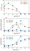 |
Fig. 1. General properties of the X-ray spectrum for beam K = 400 keV (red) and K = 800 keV (blue). Top: ratio of the luminosity radiated from the rear of the cloud and the hot spot at the front as a function of the density of the cloud. Middle: luminosity of the spectra as a function of the density. Bottom: dependence of the centroid of the X-ray energy distribution on the cloud density. The continuous and dashed lines refer to data from the transmitted and backscattered spectra. The kinetic energy of the e-beam is fully absorbed within the cloud for particle densities above 1014 cm−3. |
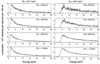 |
Fig. 2. Output X-ray spectrum from the rear of the cloud. |
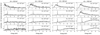 |
Fig. 3. Output X-ray spectrum from the hot spot obtained for kinetic energies of the e-beam: 200 keV, 400 keV, 800 keV, and 1.6 MeV (see top), and a media density of 1014 cm−3, 1015 cm−3, 1016 cm−3, and 1017 cm−3. No hot spot is produced for the lowest simulated density N = 1013 cm−3, nor is there any Fe Kα emission. |
The spectrum of the hot spot contains some additional interesting features, including some prominent emission lines. The Fe Kα line (6.4 keV) is observed for N > 1013 cm−3, as a strong feature in the spectrum; this line is an unresolved doublet produced in the transitions [1s2S1/2]−[2p2P1/2, 3/2] of Fe II. For e-beams with a kinetic energy of K ≥ 800 MeV and N ≥ 1016 cm−3, the Fe Kβ line at 7.1 keV is also observed. As shown in Fig. 4, the strength of the Fe Kα line decreases as the density of the cloud increases, while the strength of the Fe II Kβ line depends on the energy of the e-beam. The ratio Fe Kα/Fe Kβ also decreases with the energy of the beam. The broad iron feature at ∼6.7 keV, which is usually observed in TTSs, is only detected in a few spectra (see Fig. 5). This feature arises from very hot plasma in the hot spot at the point of impact of the e-beam. This Fe XXV feature is probably a blend of the x, y, and z lines of Fe XXV (see Phillips 2004, for a detailed description of the main transitions).
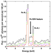 |
Fig. 4. Fe feature in the spectrum of the hot spot (see Fig. 3). Only some relevant simulations are shown. (ρ = 1016 cm s−3, K = 800 keV) is marked in black, (ρ = 1017 cm s−3, K = 800 keV) is marked in purple, (ρ = 1016 cm s−3, K = 1, 600 keV) is marked in green, and (ρ = 1017 cm s−3, K = 1600 keV) is marked in brown. |
The main features derived from this grid of simulations are listed below.
-
Fe Kα (and Kβ) emission is only observed in the spectra of the hot spot and for densities above 1014 cm−3.
-
⟨K⟩ = 400 keV maximizes the Fe Kα emission (see Fig. 5).
-
Increasing ⟨K⟩ or increasing the density of the cloudlet shifts the centroid, that is, it causes the output X-ray spectrum to become harder.
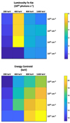 |
Fig. 5. Variation in the Fe Kα flux (top) and the energy centroid (bottom) of the X-ray spectrum with the cloud density and the mean kinetic energy of the beam < K. |
In general, this process is inefficient in terms of the X-ray radiation production compared with the input of the mechanical energy of the e-beam. As an example, in the simulation with ⟨K⟩ = 400 keV and N = 1014 cm−3, the hot spot only radiates (in the 2–30 keV range) ∼0.07% of the input mechanical luminosity of the e-beam, and the radiation from the rear of the cloudlet is ten times lower. Most of the energy of the cloudlet is diffused away by the scattered electrons, and thus, only large dense structures are efficient in the transference of the e-beam energy into X-ray radiation.
4. X-ray output from the impact of e-beams on the accretion disk
In this setup, the e-beam was assumed to impinge perpendicularly to the surface of the disk, which was stratified. The disk was modeled as a set of plane-parallel layers of increasing density to the midplane, following the vertical structure of a standard α disk (Shakura & Sunyaev 1973). The scalings were adopted from Gómez de Castro (2013). The e-ebeam impacted on the disk from the z-axis, as shown in Fig. 6, and the disk density depends on z as
 (6)
(6)
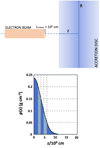 |
Fig. 6. Top: Simulation scheme. The e-beam impinges normally on the accretion disk surface. Bottom: Normalized density profile (see Eq. (6)) represented for the inner border of a sample disk with an accretion rate of 10−8 M⊙ yr−1. The structure is symmetric around the disk midplane, and only the upper part is represented. The density profile from Eq. (6) is plotted with a blue line, and the limits of the five layers implemented in the simulation are marked with dashed lines. |
with
 (7)
(7)
and
 (8)
(8)
The disk temperature is given by
 (9)
(9)
The numerical code PENELOPE was not designed to work with a density profile along the z-axis of the irradiated sample. To overcome this problem, the disk was implemented as set of plane-parallel layers of uniform density. The exponential profile described in Eq. (5) was reproduced by ten layers, as shown in Fig. 6, and the mean density changed by ∼25% between the layers.
The simulation grid is summarized in Table 1. As in Sect. 3, the radius of the e-beam was assumed to be 105 cm, and the disk composition was set to solar abundances. The output spectra obtained for an e-beam with ⟨K⟩ = 800 keV are represented in Figs. 7 (transmitted) and 8 (hot spot). For the range of mechanical luminosities of the e-beam studied in this work (∼10−1 − ∼10−4 L⊙), the X-ray luminosity increases linearly with the e-beam mechanical luminosity. Only spectra corresponding to a sample luminosity (2 × 10⁻³ L⊙) are therefore represented in the figures.
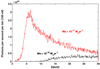 |
Fig. 7. Transmitted X-ray spectrum. Simulation with an e-beam luminosity of 2 × 10⁻³ L⊙. |
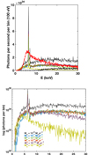 |
Fig. 8. Output X-ray spectrum of the hot spot. Top panel: comparison between the X-ray spectra of the hot spot (thin lines) with the transmitted spectra (thick dashed lines; see Fig. 7). All the spectra are plotted on the same scale. The Fe feature in the backscattered spectrum at high accretion rates is strong. Bottom panel: X-ray spectra of the hot spot on a logarithmic scale. The e-beam properties are K = 800 keV and 2 × 10⁻³ L⊙. |
Network of simulations of the interaction of the e-beams with the inner disk*.
As expected, the e-beam is absorbed in high-density environments. This translates into accretion rates Ma > 10−10 M⊙ yr−1 in the accretion disk scenario. The transmitted spectrum is only observed for the most rarified accretion disks, and the cutoff energy shifts to higher energies as the accretion rate increases (see Fig. 7). Again, no spectral features are observed in the transmitted spectrum.
The spectrum of the hot spot displays a prominent Fe Kα feature and X-ray continuum emission whose properties depend on the accretion rate, that is, on the density and stratification of the disk (see Fig. 8).
To study the dependence of the spectrum on the e-beam energy, an additional set of simulations was run for an accretion rate of 10−7 M⊙ yr−1 and ⟨K⟩ = 40, 100, 200, 400, 800, and 1600 Kev. As expected, as the e-beam mean kinetic energy rises, the Fe feature becomes stronger, and the centroid of the backscattered spectrum moves to higher energies (see Fig. 9).
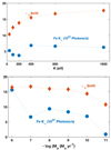 |
Fig. 9. Variation in the centroid of the X-ray spectrum and the Fe Kα flux with top the average energy of the e-beam (for Ma = 10−7 M⊙ yr−1) and bottom the accretion rate (for K = 800 keV). |
The trends described in this section can be summarized as follows:
-
The Fe Kα (and Kβ) emission is very weak or absent in the transmitted spectra.
-
Increasing the mean kinetic energy (⟨K⟩) of the e-beam or increasing the density of the medium shifts the centroid of the spectrum to higher energies.
The e-beam is also highly directive. The size of the hot spot at the point of impact is comparable to the beam radius, and the radiative output scales linearly with the surface of spot.
5. Interpretation of RY Tau flares
RY Tau is one of the best-studied accreting TTSs at X-rays. Its X-ray spectrum is known to vary from quiescence to a flare state from the observations carried out with the Chandra and the XMM-Newton satellites (see Skinner et al. 2016). We used the XMM-Newton observations to evaluate whether the reported Fe Kα emission during flares can be produced from the hot spots generated during the flares.
RY Tau was observed in September 2000 and in August 2013 (see Table 2), but no significant flaring activity was detected in 2000 (Güdel et al. 2007). We retrieved the data obtained with the European Photon Imaging Camera (EPIC) pn instrument in 2013 from the archive, id. 0722320101, and processed them using the XMM-Newton Science Analysis System (SAS 19.0.0). The spectrum was analyzed using XSPEC 12.11.1.
XMM-Newton EPIC observations of RY Tau.
Following an approach similar to that of Skinner et al. (2016), the spectra were extracted using PN cleaned and filtered for background event files. First, the event files were created by removing high-energy proton intervals at the end of the exposure and by time-filtering to cover the quiescent and flare periods. The quiescent spectrum was produced using events from 0.0 to 20.0 ks and from 45.0 to 90.0 ks, and the flare spectrum was produced using events from 20.0 to 45.0 ks. Then, source and background spectra were extracted using the evselect task. After this, the source spectra were obtained using a computed redistribution matrix and the proper ancillary file. Finally, the spectra were rebinned using the specgroup task. The quiescent spectrum was rebinned in order to have at least 40 counts for each background-subtracted spectral channel. The flare spectrum was then rebinned to group it in exactly the same way as the source spectrum. They are plotted in Fig. 10 and are similar to those in Fig. 3 of Skinner et al. (2016).
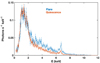 |
Fig. 10. X-ray spectrum of RY Tau obtained with the instrument EPIC on board the XMM-Newton satellite in August 2013 (observation ID: 0722320101). The X-ray light curve has been analyzed to discriminate the flare spectrum from the quiescence spectrum. |
During the flare, the X-ray flux increases at energies above 2 keV. The prominent Fe Kα emission is also clearly apparent, as is the Fe XXV feature. The spectral energy distribution of the X-ray emission during the flare is represented in Fig. 11. To obtain it, the quiescence spectrum was subtracted from the flare spectrum, but only energy bins with signal-to-noise ratio (S/N), S/N ≥ 3 were considered. The error bars were computed using the standard expression for the linear propagation of errors,
 (10)
(10)
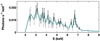 |
Fig. 11. Spectral distribution of the X-ray radiation produced by the flare. Data points with S/N ≥ 3 are marked in black, and those with S/N ≥ 2 are shown in gray. The green line is plotted to guide the eye to the overall energy distribution, where the prominent Fe Kα and Fe XXV features are readily recognized. |
with σflare and σquiescence the variances of the flare, and quiescence spectra provided by XSPEC (for obvious reasons, some data points have σexcess < 3).
The Fe Kα flux during the flare was computed using the XPEC routines and was found to be 0.87 × 10⁻¹³ erg s−1 cm−2, which accounts for a total luminosity of the line of 2.01 × 1029 erg s−1, using the Gaia parallax of RY Tau (7.2349 mas) for the calculation. This luminosity is equivalent to a grand total of 1.96 × 1037 Fe Kα photons per second during the flare. This value should be divided by 4π to compare it with the results from the simulations described in the previous sections.
This luminosity cannot be accounted for by the impact of relativistic electrons on the diffuse environment around the loops (either the funnel flows or the dense stellar corona) because as shown in Sect. 3, Fe Kα radiation is only produced when the density is very high (> 1014 cm−3). However, the observed Fe Kα emission could arise from hot spots on the accretion disk generated at the impact point of the e-beams from the flares.
The environment around an active TTS such as RY Tau is strongly magnetized and has a complex topology that easily produces magnetic reconnection in many different regions. A simplified approach to the overall topology is displayed in Fig. 12 (after Gómez de Castro et al. 2016). In the classical TTS evolutionary state, the stellar field is connected with the disk field to the point that stellar rotation is locked to the Keplerian velocity of the inner border of the disk. The dashed lines mark the limit between the disk-dominated and the star-dominated regions. Overplotted on this magnetic sketch, the results of numerical simulations of this interaction (Gómez de Castro & von Rekowski 2011) are shown in the figure. The green-brown shadowed regions are locations in which magnetic reconnection heats the gas and produces ultraviolet radiation. In this environment, the most obvious region to have frequent and strong reconnection events is the inner border of the disk. However, the geometry is not clear; reconnection may occur above the disk and produce e-beams that impact on the disk surface (as simulated in Sect. 4). E-beams may be generated just at the inner border and interact with specific layers of the disk vertical structure, however. These two simple possibilities are marked in Fig. 12 as options A and B, respectively. Although the geometry is much more complex in general, we kept it simple for this prospective work and evaluated whether the Fe Kα emission detected during the flare is compatible with the radiation produced in the propagation of the high-energy e-beams produced during large flares within the disk.
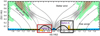 |
Fig. 12. Map of the C III] (191 nm) emissivity caused by the star-disk interaction from MHD simulations of the disk-star interaction (Gómez de Castro & von Rekowski 2011). At the top, we plot the main components of the TTSs environment and the magnetic structure. The magnetic field is represented by solid lines, and the very thick line marks the connection between the star and the inner border of the disk. The stellar interaction with the infalling magnetized plasma drives the outflow and generates reconnection layers (dashed lines). |
According to the simulations in Sect. 4, the Fe Kα luminosity produced by an e-beam impacting perpendicularly to the accretion disk depends on the accretion rate, which has been measured to range between 0.91 × 10⁻⁷ M⊙ yr−1 and 0.50 × 10⁻⁷ M⊙ yr−1 for RY Tau (Alcalá et al. 2021). For these rates, the predicted line luminosity ranges between 3.4 × 1037 photons s−1 and 4.7 × 1037 photons s−1 for a mechanical luminosity of the e-beam of 0.1 L⊙, which is within a factor of two of the detected values. This factor could easily be accommodated when the luminosity of the flare or the surface of the hot spot were reduced.
In the case of a lateral impact (option B in Fig. 12), the particle density of the midplane is expected to range between 0.77 × 1016 cm−3 and 1.13 × 1016 cm−3 (see Eq. (8)), and thus, according to Fig. 5, the Fe Kα emission is predicted to range between 3 × 1036 photons s−1 and 6 × 1036 photons s−1, depending on the mean kinetic energy of the electrons, for an e-beam of mechanical luminosity of 0.02 L⊙. The Fe Kα luminosity scales linearly with the mechanical luminosity, and therefore, a strong flare with a luminosity 0.1 L⊙ could produce an emission similar to the observed emission.
In summary, the Fe Kα emission detected in RY Tau during the large flare in 2013 can easily be accounted for by the propagation of the e-beams generated during the flare within the inner border of the disk.
6. Conclusions
The X-ray observations of the TTSs have shown that some classical TTSs experience very strong flares that are associated with the release of magnetic energy during the reconnection of very long magnetic loops that extend up to a few stellar radii. These strong reconnection events might be produced when stellar loops meet the inner border of the disk. A characteristic of these flares is the detection of Fe Kα emission, which, in the case of RY Tau, reaches a line luminosity of 1.96 × 1037 Fe Kα photons s−1 during the flare. We showed that this emission can naturally be explained by the X-ray radiation produced at the impact point of the high-energy electrons that are released during the reconnection event on the accretion disk.
We also included a broad network of numerical simulations of the expected X-ray radiative output in this context to aid the interpretation of X-ray observations of TTSs during flares.
We concentrated on modeling the radiative output from large flares that meet the inner border of the disk, but similar phenomena (and Fe Kα emission) might be produced by the impact of the e-beams on the stellar surface. In all cases, very strong flare luminosities are required to reproduce the observed Fe Kα flux, however.
The Monte Carlo algorithm implemented in PENELOPE incorporates a “mixed” scattering model for the simulation of electron and positron transport. Hard interactions, with scattering angle and/or energy loss greater than preselected cutoff values are simulated in detail, by using simple analytical differential cross sections for the different interaction mechanisms and exact sampling methods. Soft interactions, with scattering angle or energy loss less than the corresponding cutoffs, are described by means of a multiple scattering approach. The code is user-friendly and incorporates photon cross-section data from the EPDL97 which includes new libraries for the low-energy photon cross-sections, such as XCOM and EPDL97. The code is available at the web site of the International Atomic Energy Agency (http://www.nea.fr/lists/penelope.html).
The code is also widely used in the medical community, and, for instance, Sung-Joon et al. (2004) recently verified it for clinical dosimetry of high-energy (10 keV–150 keV) electron and photon beams.
Acknowledgments
This work has been partially funded by the Ministry of Science, Innovation and Universities of Spain through the grant with reference: PID2020-116726RB-I00.
References
- Alcalá, J. M., Gangi, M., Biazzo, K., et al. 2021, A&A, 652, A72 [NASA ADS] [CrossRef] [EDP Sciences] [Google Scholar]
- Anders, E., & Ebihara, M. 1982, Geochim. Cosmochim. Acta, 46, 2363 [NASA ADS] [CrossRef] [Google Scholar]
- Antonicci, A. 2004, PhD Thesis, Universidad Complutense de Madrid, Spain [Google Scholar]
- Antonicci, A., & Gómez de Castro, A. I. 2005, A&A, 432, 443 [NASA ADS] [CrossRef] [EDP Sciences] [Google Scholar]
- Baró, J., Sempau, J., Fernandez-Varea, J., & Salvat, F. 1994, Nucl. Instrum. Method, B84, 465 [CrossRef] [Google Scholar]
- Battaglia, M., Kontar, E. P., & Motorina, G. 2019, ApJ, 872, 204 [CrossRef] [Google Scholar]
- Czesla, S., & Schmitt, J. H. M. M. 2010, A&A, 520, A38 [NASA ADS] [CrossRef] [EDP Sciences] [Google Scholar]
- Drake, J. J., Ercolano, B., & Swartz, D. A. 2008, ApJ, 678, 385 [NASA ADS] [CrossRef] [Google Scholar]
- Dyda, S., Lovelace, R. V. E., Ustyugova, G. V., et al. 2015, MNRAS, 450, 481 [Google Scholar]
- Favata, F., Flaccomio, E., Reale, F., et al. 2005, ApJS, 160, 469 [CrossRef] [Google Scholar]
- Gómez de Castro, A. I. 2013, in Planets, Stars and Stellar Systems. Volume 4: Stellar Structure and Evolution, eds. T. D. Oswalt, & M. A. Barstow, 4, 279 [CrossRef] [Google Scholar]
- Gómez de Castro, A. I., & Antonicci, A. 2006, Astron. Nachr., 327, 989 [CrossRef] [Google Scholar]
- Gómez de Castro, A. I., & von Rekowski, B. 2011, MNRAS, 411, 849 [CrossRef] [Google Scholar]
- Gómez de Castro, A. I., Gaensicke, B., Neiner, C., & Barstow, M. A. 2016, J. Astron. Telesc. Instrum. Syst., 2, 041215 [CrossRef] [Google Scholar]
- Güdel, M., Briggs, K. R., Arzner, K., et al. 2007, A&A, 468, 353 [Google Scholar]
- Günther, H. M., & Schmitt, J. H. M. M. 2008, A&A, 481, 735 [NASA ADS] [CrossRef] [EDP Sciences] [Google Scholar]
- Heyvaerts, J., Priest, E. R., & Rust, D. M. 1977, ApJ, 216, 123 [Google Scholar]
- Jardine, M., Collier Cameron, A., Donati, J. F., Gregory, S. G., & Wood, K. 2006, MNRAS, 367, 917 [NASA ADS] [CrossRef] [Google Scholar]
- Kastner, J. H., Huenemoerder, D. P., Schulz, N. S., Canizares, C. R., & Weintraub, D. A. 2002, ApJ, 567, 434 [Google Scholar]
- Kulkarni, A. K., & Romanova, M. M. 2013, MNRAS, 433, 3048 [NASA ADS] [CrossRef] [Google Scholar]
- Lamzin, S. A. 1998, Astron. Rep., 42, 322 [NASA ADS] [Google Scholar]
- López-Martínez, F., & Gómez de Castro, A. I. 2014, MNRAS, 442, 2951 [CrossRef] [Google Scholar]
- Morrison, R., & McCammon, D. 1983, ApJ, 270, 119 [Google Scholar]
- Oka, M., Fujimoto, M., Nakamura, T. K. M., Shinohara, I., & Nishikawa, K. I. 2008, Phys. Rev. Lett., 101, 205004 [NASA ADS] [CrossRef] [Google Scholar]
- Phan-Bao, N., Lim, J., Donati, J.-F., Johns-Krull, C. M., & Martín, E. L. 2009, ApJ, 704, 1721 [NASA ADS] [CrossRef] [Google Scholar]
- Phillips, K. J. H. 2004, ApJ, 605, 921 [NASA ADS] [CrossRef] [Google Scholar]
- Preibisch, T., Kim, Y.-C., Favata, F., et al. 2005, ApJS, 160, 401 [NASA ADS] [CrossRef] [Google Scholar]
- Romanova, M. M., Ustyugova, G. V., Koldoba, A. V., & Lovelace, R. V. E. 2012, MNRAS, 421, 63 [NASA ADS] [Google Scholar]
- Schmitt, J. H. M. M., Robrade, J., Ness, J. U., Favata, F., & Stelzer, B. 2005, A&A, 432, L35 [NASA ADS] [CrossRef] [EDP Sciences] [Google Scholar]
- Shakura, N. I., & Sunyaev, R. A. 1973, A&A, 24, 337 [NASA ADS] [Google Scholar]
- Skinner, S. L., Audard, M., & Güdel, M. 2016, ApJ, 826, 84 [Google Scholar]
- Sung-Joon, Y., Brezovich, I., Pareek, P., & Naqvi, S. 2004, Phys. Med. Biol., 49, 387 [NASA ADS] [CrossRef] [Google Scholar]
- Tsuboi, Y., Koyama, K., Murakami, H., et al. 1998, ApJ, 503, 894 [NASA ADS] [CrossRef] [Google Scholar]
- Tsujimoto, M., Feigelson, E. D., Grosso, N., et al. 2005, ApJS, 160, 503 [CrossRef] [Google Scholar]
- Villebrun, F., Alecian, E., Hussain, G., et al. 2019, A&A, 622, A72 [NASA ADS] [CrossRef] [EDP Sciences] [Google Scholar]
- Wolk, S. J., Harnden, F. R. J., Flaccomio, E., et al. 2005, ApJS, 160, 423 [NASA ADS] [CrossRef] [Google Scholar]
- Yang, H., & Johns-Krull, C. M. 2011, ApJ, 729, 83 [Google Scholar]
All Tables
All Figures
|
Fig. 1. General properties of the X-ray spectrum for beam K = 400 keV (red) and K = 800 keV (blue). Top: ratio of the luminosity radiated from the rear of the cloud and the hot spot at the front as a function of the density of the cloud. Middle: luminosity of the spectra as a function of the density. Bottom: dependence of the centroid of the X-ray energy distribution on the cloud density. The continuous and dashed lines refer to data from the transmitted and backscattered spectra. The kinetic energy of the e-beam is fully absorbed within the cloud for particle densities above 1014 cm−3. |
| In the text | |
|
Fig. 2. Output X-ray spectrum from the rear of the cloud. |
| In the text | |
|
Fig. 3. Output X-ray spectrum from the hot spot obtained for kinetic energies of the e-beam: 200 keV, 400 keV, 800 keV, and 1.6 MeV (see top), and a media density of 1014 cm−3, 1015 cm−3, 1016 cm−3, and 1017 cm−3. No hot spot is produced for the lowest simulated density N = 1013 cm−3, nor is there any Fe Kα emission. |
| In the text | |
|
Fig. 4. Fe feature in the spectrum of the hot spot (see Fig. 3). Only some relevant simulations are shown. (ρ = 1016 cm s−3, K = 800 keV) is marked in black, (ρ = 1017 cm s−3, K = 800 keV) is marked in purple, (ρ = 1016 cm s−3, K = 1, 600 keV) is marked in green, and (ρ = 1017 cm s−3, K = 1600 keV) is marked in brown. |
| In the text | |
|
Fig. 5. Variation in the Fe Kα flux (top) and the energy centroid (bottom) of the X-ray spectrum with the cloud density and the mean kinetic energy of the beam < K. |
| In the text | |
|
Fig. 6. Top: Simulation scheme. The e-beam impinges normally on the accretion disk surface. Bottom: Normalized density profile (see Eq. (6)) represented for the inner border of a sample disk with an accretion rate of 10−8 M⊙ yr−1. The structure is symmetric around the disk midplane, and only the upper part is represented. The density profile from Eq. (6) is plotted with a blue line, and the limits of the five layers implemented in the simulation are marked with dashed lines. |
| In the text | |
|
Fig. 7. Transmitted X-ray spectrum. Simulation with an e-beam luminosity of 2 × 10⁻³ L⊙. |
| In the text | |
|
Fig. 8. Output X-ray spectrum of the hot spot. Top panel: comparison between the X-ray spectra of the hot spot (thin lines) with the transmitted spectra (thick dashed lines; see Fig. 7). All the spectra are plotted on the same scale. The Fe feature in the backscattered spectrum at high accretion rates is strong. Bottom panel: X-ray spectra of the hot spot on a logarithmic scale. The e-beam properties are K = 800 keV and 2 × 10⁻³ L⊙. |
| In the text | |
|
Fig. 9. Variation in the centroid of the X-ray spectrum and the Fe Kα flux with top the average energy of the e-beam (for Ma = 10−7 M⊙ yr−1) and bottom the accretion rate (for K = 800 keV). |
| In the text | |
|
Fig. 10. X-ray spectrum of RY Tau obtained with the instrument EPIC on board the XMM-Newton satellite in August 2013 (observation ID: 0722320101). The X-ray light curve has been analyzed to discriminate the flare spectrum from the quiescence spectrum. |
| In the text | |
|
Fig. 11. Spectral distribution of the X-ray radiation produced by the flare. Data points with S/N ≥ 3 are marked in black, and those with S/N ≥ 2 are shown in gray. The green line is plotted to guide the eye to the overall energy distribution, where the prominent Fe Kα and Fe XXV features are readily recognized. |
| In the text | |
|
Fig. 12. Map of the C III] (191 nm) emissivity caused by the star-disk interaction from MHD simulations of the disk-star interaction (Gómez de Castro & von Rekowski 2011). At the top, we plot the main components of the TTSs environment and the magnetic structure. The magnetic field is represented by solid lines, and the very thick line marks the connection between the star and the inner border of the disk. The stellar interaction with the infalling magnetized plasma drives the outflow and generates reconnection layers (dashed lines). |
| In the text | |
Current usage metrics show cumulative count of Article Views (full-text article views including HTML views, PDF and ePub downloads, according to the available data) and Abstracts Views on Vision4Press platform.
Data correspond to usage on the plateform after 2015. The current usage metrics is available 48-96 hours after online publication and is updated daily on week days.
Initial download of the metrics may take a while.