| Issue |
A&A
Volume 622, February 2019
|
|
|---|---|---|
| Article Number | L11 | |
| Number of page(s) | 7 | |
| Section | Letters to the Editor | |
| DOI | https://doi.org/10.1051/0004-6361/201834663 | |
| Published online | 11 February 2019 | |
Letter to the Editor
Carbon 12C/13C isotope ratio of α Aurigae revised
Leibniz-Institute for Astrophysics Potsdam (AIP), An der Sternwarte 16, 14482 Potsdam, Germany
e-mail: dsablowski@aip.de
Received:
11
January
2019
Accepted:
30
January
2019
Context. Capella (α Aur) is one of the few binaries in the sky with two cool giant stars. With spectral types of G8III and G0III, the two components appear at different but distinct stages in their evolution. The G0 secondary star is a Hertzsprung-gap giant, and the G8 primary star is thought to be a clump giant.
Aims. We present a new measure of the carbon 12C/13C isotope ratio of the primary component of Capella using high-resolution R ≈ 250 000 spectra obtained with the Potsdam Echelle Polarimetric and Spectroscopic Instrument (PEPSI) with both the Vatican Advanced Technology Telescope (VATT) and the Large Binocular Telescope (LBT).
Methods. Signal-to-noise ratios of up to 2 700 were obtained by averaging nightly spectra. These average spectra were used to disentangle the two binary components. The isotope ratio was derived with the use of spectrum synthesis from the CN lines at 8004 Å.
Results. We found that the 12C/13C ratio of the primary component of Capella is 17.8 ± 1.9. Our measurement precision is now primarily limited by the spectral-line data and by the grid-step size of the model atmospheres rather than the data. The separated spectrum of the secondary component does not show distinguishable 12CN and 13CN lines because of its vsini and higher temperature.
Conclusions. Our new 12C/13C value is significantly lower than the previous value of 27 ± 4 but now agrees better with the recent model prediction of 18.8–20.7.
Key words: stars: evolution / binaries: spectroscopic / methods: observational / techniques: spectroscopic
© ESO 2019
1. Introduction
Stellar evolution is traced by the carbon, nitrogen, and oxygen (CNO) abundances and in particular by the 12C/13C isotope ratio (e.g., Shetrone 2003; Szigeti et al. 2018) because carbon will be converted into nitrogen and the 12C/13C ratio will be lowered over time by molecular CN processing (also CH and CO). The surface CNO abundances also depend on the mixing process (e.g., Mikolaitis et al. 2012; Drazdauskas et al. 2016; Tautvaisiene et al. 2016). Moreover, the abundances are not only scaled to stellar nucleosynthesis and mixing, but also to galactic chemical evolution (e.g., Allende Prieto et al. 2004). Previous isotopic measurements (see Lambert & Ries 1981) indicate that the observed ratios for G–K giants are of about 10–30, which is significantly lower than the presumed initial (solar) ratio of about 90 (e.g. Anders & Grevesse 1989; Jewitt et al. 1997). Iben (1964) made the first theoretical prediction of evolution-caused changes of isotopic abundances from the reaction 12CN(p, γ)13N(β+, ν)13C(p, γ)14N (see also Henry et al. 2000; Yang et al. 2017). This reaction suggested that 13C may be used as an observational tracer once it has been brought up to the surface. It is therefore expected that the 12C/13C ratio decreases and the 14N/15N ratio increases with stellar evolution.
The main mechanism of mixing in stars is convection. However, stars that gain their energy primarily by the CNO cycle have radiative envelopes during their main-sequence lifetime. After hydrogen is exhausted in the core, the core contracts and heats the outer layers. A convection layer at the surface of the star is established and penetrates the interior of the star. As a consequence, processed material is transported to the surface. This is referred to as the first dredge-up, and it occurs when the star enters the Hertzsprung gap in the Hertzsprung-Russel (HR) diagram. To explain stars with very low carbon isotope ratios, additional mixing processes were suggested. The rotation-induced meridional mixing can provide mixing even during the main-sequence phase (e.g., Drazdauskas et al. 2016; Charbonnel & Lagarde 2010). The nature of further mixing processes after the first dredge-up is still debated (e.g., Pinsonneault 1997; Charbonnel & Lagarde 2010; Hedrosa et al. 2013).
In this respect, binaries are of special interest because they consist of stars of the same age and same initial chemical composition that are at different stages of evolution, if of different mass. Capella (G8III is the primary and G0III is the secondary) is such a system. The combination of the many pieces known for this system, in particular stellar masses at the sub-percent precision (Weber & Strassmeier 2011), resulted in rather detailed and precise models of stellar evolution for both components (Torres et al. 2015). In spite of the small mass difference of only about 3.5 ± 0.4% between the two Capella components, they are at very different stages of evolution. The rapidly rotating secondary has just left the main sequence and is on its short path through the Hertzsprung gap, while the primary may be already near the end of the He-core burning phase. Hence, we expect to see significant differences in the CNO elements and their isotopes at the surface. The 12C/13C ratio of Capella was measured for the more evolved primary component by Tomkin et al. (1976) to be 27 ± 4. This value is now over 40 years old, and its discrepancy compared to the model values presented by Torres et al. (2015) led to the present study.
We use the CN molecular lines around 8004 Å for the isotope measurement. This region is the least blended and best accessible wavelength region in the optical for this type of analysis. It displays one line that is purely due to 12CN and one line that is purely due to 13CN. New observations are presented in Sect. 2, the data reduction and spectrum disentangling is described in Sect. 3, and our spectrum-synthesis analysis is given in Sect. 4. Our conclusions are summarized in Sect. 5.
2. Observations
The observations were carried out with the Potsdam Echelle Polarimetric and Spectroscopic Instrument (PEPSI; Strassmeier et al. 2015) installed on the pier of the 2 × 8.4 m Large Binocular Telescope (LBT) on Mt. Graham, Arizona. Most of the spectra were obtained with the 1.83 m Vatican Advanced Technology Telescope (VATT), which has a 450 m fibre link to the PEPSI spectrograph at the LBT. A Cassegrain adapter on the VATT was used for target acquisition and guiding, and it also provides the feed for the entrance fibre (Sablowski et al. 2016).
PEPSI has three resolution modes related to the three fibre core diameters that feed it; see Strassmeier et al. (2018a) for a status and most recent mode description of the instrument. We used the ultra-high resolution mode with R = λ/Δλ = 250 000 (2-pixel sampling and 0.74″ sky aperture at LBT) with two pairs of 100 μm fibres and seven-slice image slicers. When fed from the VATT and used before mid-2016, PEPSI provided the same spectral resolution as when fed from the LBT, but with higher losses. After mid-2016, two new pairs of image slicers were implemented for the VATT feed. These provide an expected 2.6-pixel resolution of 200 000 with a single 3″ sky aperture with a 200 μm fibre and a 9-slice image slicer for a 2-pixel resolution of 250 000 with the same aperture and a 9-slice image slicer, but smaller slice width. The respective wavelength coverage at LBT and VATT are always identical. PEPSI has blue and red arms with three cross-dispersers (CD) in each arm. One CD in each arm can be used simultaneously.
With the double-eyed LBT the light from the fibre pair of target and sky (optionally, it can be light from a Fabry-Pérot etalon) is rendered to four image slicers via respective octagonal fibres before it enters the spectrograph. Two 10k × 10k STA1600LN CCDs with 9 μm pixel size and 16 amplifiers optimized for the blue and red arms are employed. When used with the VATT, only a single-eyed light path is available and no sky (but Fabry-Pérot light). The spectrograph is located in a pressure-controlled chamber at a constant temperature and humidity to keep the refractive index of the air inside constant. This provides a long-term radial velocity stability of about 5 m s−1.
We acquired 70 spectra in total of Capella with the red-arm CD VI (λ7355–9137 Å) between November 28, 2015 and March 15, 2017. The wavelength solution used about 3000 ThAr lines and showed an error of the fit at the image center of 5 m s−1. Consecutive single exposures obtained during the same night were averaged to obtain 12 spectra with high signal-to-noise ratio (S/N) that were then used to separate the two stellar components. These averaged spectra are listed in Table 1. The resolving power of the spectra varies according to the setup that was used, between 200k and 250k. The SN/ was measured to be about 8000 Å and is on average about 2000:1. Figure 1 plots the 12 averaged spectra in the 8004 Å region.
Overview of observations.
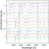 |
Fig. 1. Twelve Capella spectra that were used for the disentanglement. The bottom spectrum is the first spectrum listed in Table 1. The others are shifted in intensity by +0.2 for better visibility. The spectra are shown in laboratory wavelength scale (prior to heliocentric correction), and some telluric features are marked with vertical red lines. |
3. Data reduction and spectral disentangling
The data were reduced on a generic software platform written in C++ under Linux, called the Spectroscopic Data System (SDS). The current image processing pipeline is specifically designed to handle the PEPSI data calibration flow and image specific content and is called SDS4PEPSI. The same SDS tools can be used for spectra that are obtained with different échelle spectrographs. It provides an automated pipeline without human interaction and relies on statistical inferences and robust statistics. The software numerical toolkit and graphical interface are designed based upon Ilyin (2000). Its application to PEPSI has initially been described in Strassmeier et al. (2018b), and its complete description will be presented in Ilyin (in prep.).
The standard steps of image processing include the following: bias subtraction and variance estimation of the source images, super-master flat-field correction for the CCD spatial noise, échelle order definition from the tracing flats, scattered light subtraction, wavelength solution for the ThAr images, optimal extraction of image slicers and cosmic spike elimination of the target image, wavelength calibration and merging slices in each order, normalization to the master flat-field spectrum to remove CCD fringes and blaze function, a global 2D fit to the continuum of the normalized image, and rectification of all spectral orders in the image to a 1D spectrum for a given cross-disperser. The continuum of the final spectra in the time series was corrected for with the use of the mean spectrum. The weighted average of all spectra was normalized to the continuum to eliminate any residual effects in the continuum. The ratio of each individual spectrum and the mean is then used to fit a smoothing spline that constitutes the improved continuum for the individual spectra.
The disentangling code Spectangular was presented by Sablowski & Weber (2017) and is based on singular-value decomposition (SVD) in the wavelength domain. It does not require correct input radial velocities (RVs) because it optimizes them during a full disentangling run. To apply this approach, it is necessary to use observations that are significantly spread over an orbital period. Because SVD requires an overdetermined set of equations, the minimum input is at least three spectra for two components. The Capella spectra used for the disentangling are shown in Fig. 1. Only a small wavelength fraction is plotted. These spectra are not well distributed throughout the orbit (Porb = 104 d, see Table 1 for covered phases ϕ), but the small RV shifts between the spectra were sufficient for the algorithm to extract the individual components (see also Appendix B). The disentangling by the use of poorly sampled orbit was studied in Sablowski & Weber (2017). Furthermore, the disentangling code requires a priori knowledge of the light ratio of the two components in the wavelength range under consideration. We adopted the ratio of 1.118 (G8/G0) from Huby et al. (2013; see also Appendix A).
An additional bonus from this disentangling process is that the telluric spectrum is removed. Water vapor lines, which we call tellurics, further complicate the analysis as well as the disentangling process because they can vary dramatically in strength (and they even slightly vary in RV). This is shown in Fig. 1 for a pair of telluric lines at wavelengths of about 8007.6 Å and for a line at 8000.3 Å. In order to preserve the flux in the wavelength pixels that are affected by tellurics, we did not apply the heliocentric correction before disentangling. This leads to a fixed position of tellurics in wavelength space. The high variability in the strength of these lines leads to a strong suppression in the separated spectra, which is due to the least-squares nature of the SVD solution. We then used the residuals from the separated spectra to identify the contribution of tellurics in each spectrum. These residuals were then approximated by a proper spline and corrected in the individual observed spectra. A second run of the entire disentangling process resulted in component spectra with negligible telluric contamination. For more details on this procedure, we refer to a forthcoming paper by Sablowski et al. (2019) and to the appendix. The final result of the separated spectra for the primary of Capella is shown in Fig. 2.
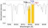 |
Fig. 2. Separated spectra of the G8III primary for the 8004 Å wavelength region of Capella. Light gray vertical lines define three continuum points, and the orange regions indicate the two fit regions for the spectrum synthesis. |
4. Analysis
For the carbon isotope ratio (CIR) we employed Spectroscopy Made Easy (SME; Valenti & Piskunov 1996; Piskunov & Valenti 2017) for a spectrum synthesis under local thermodynamical equilibrium (LTE) together with a grid of spherical model atmospheres from MARCS (Gustafsson et al. 2008) for giant stars as provided with the SME code. Because SME is not designed for individual isotope synthesis, we applied the following procedure. First, we fixed the stellar parameters to the values given in Table 2 (as derived by Takeda et al. 2018; Torres et al. 2015), but let the carbon abundance remain a free parameter. As a result of the high resolution of the spectra, the broadening values had to be reduced slightly compared to those determined by Takeda et al. (2018) and Torres et al. (2015). However, they are within the errors of the given values. These values were obtained by a synthesis of a few isolated lines, see Fig. 3. The orbital sampling in other wavelength regions is not sufficient for disentangling. We were therefore unable to determine the atmospheric parameters. Second, we fit the one line region that is solely due to 12CN while masking out all the other nearby lines. Third, we fit the other line region that is solely due to 13CN in the adjacent wavelength bin, again ignoring all the other lines (the fit regions are indicated as shaded areas in Fig. 2a). Based on these fits, we found a pseudo- 12CN and 13CN abundance from which we obtained the carbon isotope ratio. The resulting best fits for both isotopes are shown in Fig. 4 along with their 3σ deviations.
Stellar parameters for the Capella primary.
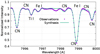 |
Fig. 3. Synthesis for refining the values of the broadening mechanisms by a few isolated lines within the separated region. The final values are ξt = 1.39 km s−1, ζ = 6.0 km s−1, and v sin i = 3.8 km s−1. |
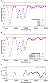 |
Fig. 4. Panel a: result from the spectrum synthesis fitting with SME. The observations are shown as dots, and we plot the best fits as blue and green lines for the 12CN and 13CN line region, respectively. This suggests an isotope ratio of 17.8 ± 1.9. The synthetic spectra for ±3σ deviations are shown as orange and red lines, respectively. Panel b: spectrum synthesis with MOOG for consistency of the spectral fitting by SME. See text for the parameters of the underlying MARCS model. Panel c: observations minus synthesis (O-S) for the MOOG synthesis. Error bars corresponds to an S/N of 1000. |
We initially implemented the line list from Carlberg et al. (2012) for the SME synthesis. However, another small blend became obvious from our spectra. It is identified with a red thick mark in Fig. 2. This line is identified in VALD-3 as Fe I 8005.0490 Å (Kurucz 2005) with an excitation potential χ = 5.58 eV and a transition probability log gf = −5.52. We added it to the Carlberg et al. (2012) list and give the full line list and its parameters in Table 3.
Line data for the synthesis.
We note that the precision of our isotope ratio is no longer limited by the data because of its high resolution, high S/N, and a continuum setting that is probably better than 0.1%. It turned out that the achievable precision is limited more by the atomic and molecular line data, and probably even more significantly, by the assumptions and grid resolutions of the model atmosphere. Tests were made by measuring the isotope ratio for synthetic spectra from multiple stellar parameters altered by the various grid resolutions and the measurement uncertainties given by Takeda et al. (2018) and Torres et al. (2015). SME provides the logarithmic abundances together with their errors, which for the best fit (stellar parameters from Table 2) correspond to log AC12 = −3.18 ± 0.000658 and log AC13 = −4.43 ± 0.04598.
For a consistency check of the applied method in SME, we generated synthetic spectra with MOOG (Sneden 1973), which can distinguish between the isotopes. These spectra were created with the same parameters as used in SME. Parameters of the MARCS model selected for the synthesis are Teff = 5000 K, log g = 2.5, [Fe/H] = 0.00, and ξt = 2.0 km s−1. A good agreement is shown by the comparison with the observations in Fig. 4b. The slightly broader lines originate from the higher ξt of 2.0 km s−1 of this model. Therefore, we also used the model with ξt = 1.0 km s−1 and computed synthetic spectra with different carbon isotope ratios (CIR). The root mean square (rms) between these spectra and the observations are shown in Fig. 5. The solid line represents a fit of an asymmetric parabola. The minima are in a very good agreement with the CIR value obtained by the fit with SME.
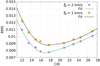 |
Fig. 5. rms between synthesized spectra from MOOG vs. CIR with the use of MARCS models (see text) with ξt = 1.0 km s−1and ξt = 2.0 km s−1, respectively. |
As described above, our analysis is limited to the models and line data. This is shown in Fig. 4c, where we plot the differences between the observations and the synthesis by MOOG with the obtained CIR.
Because the spectra from both codes agree well, we were confident to use the errors provided by the synthesis fitting in SME. The error of the isotope ratio was calculated according to the error propagation of the exponential function (e.g., Bevington & Robinson 1992) r = 10u and σr = ln10 ⋅ rσu, where r is the isotopic ratio, u = log AC12 − log AC13 and  . The resulting value is AC12/AC13 = 17.8 ± 1.9.
The separated spectrum of the secondary (see Fig. B.1c) does not show separable signatures of the 12CN and 13CN 8004 Å lines. This is probably due to its higher temperature and much larger vsini (see also Appendix B).
5. Summary and conclusion
We provided new measurement of the carbon 12C/13C isotope ratio of the Capella primary and found it to be 17.8 ± 1.9. The assigned error is mostly due to uncertainties of the molecular line data and the grid-step-size of the underlying atmospheric models rather than the data. This new ratio is significantly lower than the value of 27 ± 4 originally measured by Tomkin et al. (1976) using a curve-of-growth analysis. Torres et al. (2009) have pointed out that Tomkin’s value was derived with an incorrect light ratio between the two stellar components. They estimated that the equivalent width measurements of the CN lines reported by Tomkin et al. (1976) were underestimated by about 6–11% as a result of this effect. Because the equivalent widths were used strictly differentially, we second the statement of Torres et al. (2009) that it introduced only a small error that is likely within the error bars already given. The difference to our new ratio therefore likely originates from the improvement of the data, the synthesis analysis, and better spectral-line data.
Although our new isotope ratio is now in a better agreement with theoretical expectations of 20.7 by Torres et al. (2015) based on MESA stellar evolution models, it is now (marginally) below the predictions if at an age of 588.5 Myr (see Paxton et al. 2013). The earlier prediction by Torres et al. (2009) was based on models from Claret (2004) and Young & Arnett (2005), which were all in the range of 18.88–19.60.
Acknowledgments
We thank the anonymous referee for the constructive comments that helped to improve the content of this study. We also thank our colleagues Gohar Harutyunyan, Arto Järvinen, and the developer of MOOG, Christopher A. Sneden, as well as the developers of SME, Nikolai Piskunov and Jeff Valenti, for their kind support to get the synthesis codes MOOG and SME running. This work is based on data acquired with PEPSI at the Large Binocular Telescope (LBT) and with the Vatican Advanced Technology Telescope (VATT). The LBT is an international collaboration among institutions in the United States, Italy, and Germany. LBT Corporation partners are the University of Arizona on behalf of the Arizona university system; Istituto Nazionale di Astrofisica, Italy; LBT Beteiligungsgesellschaft, Germany, representing the Max-Planck Society, the Leibniz-Institute for Astrophysics Potsdam (AIP), and Heidelberg University; the Ohio State University; and the Research Corporation, on behalf of the University of Notre Dame, University of Minnesota, and University of Virginia. This work has made use of the VALD database, operated at Uppsala University, the Institute of Astronomy RAS in Moscow, and the University of Vienna.
References
- Allende Prieto, C., Barklem, P. S., Lambert, D. L., & Cunha, K. 2004, A&A, 420, 183 [NASA ADS] [CrossRef] [EDP Sciences] [Google Scholar]
- Anders, E., & Grevesse, N. 1989, Geochim. Cosmochim. Acta, 53, 197 [Google Scholar]
- Bagnuolo, Jr., W. G., & Sowell, J. R. 1988, AJ, 96, 1056 [NASA ADS] [CrossRef] [Google Scholar]
- Bevington, P., & Robinson, D. 1992, Data Reduction and Error Analysis for the Physical Sciences, 2nd edn. (New York: McGraw-Hill), 50 [Google Scholar]
- Carlberg, J. K., Cunha, K., Smith, V. V., & Majewski, S. R. 2012, ApJ, 757, 109 [NASA ADS] [CrossRef] [Google Scholar]
- Charbonnel, C., & Lagarde, N. 2010, A&A, 522, A10 [NASA ADS] [CrossRef] [EDP Sciences] [MathSciNet] [PubMed] [Google Scholar]
- Claret, A. 2004, A&A, 424, 919 [NASA ADS] [CrossRef] [EDP Sciences] [Google Scholar]
- Drazdauskas, A., Tautvaisiene, G., Randich, S., et al. 2016, A&A, 589, A50 [NASA ADS] [CrossRef] [EDP Sciences] [Google Scholar]
- Griffin, R., & Griffin, R. 1986, A&A, 7, 45 [Google Scholar]
- Gustafsson, B., Edvardsson, B., Eriksson, K., et al. 2008, A&A, 486, 951 [NASA ADS] [CrossRef] [EDP Sciences] [Google Scholar]
- Hedrosa, R. P., Abia, C., Busso, M., et al. 2013, ApJ, 768, L11 [NASA ADS] [CrossRef] [Google Scholar]
- Hege, E. K., Hubbard, E. N., Cocke, W. J., et al. 1983, Lowell Obs. Bull., 9, 185 [NASA ADS] [Google Scholar]
- Henry, R. B. C., Edmunds, M. G., & Köppen, J. 2000, ApJ, 541, 660 [NASA ADS] [CrossRef] [Google Scholar]
- Huby, E., Duchêne, G., Marchis, F., et al. 2013, A&A, 560, A113 [NASA ADS] [CrossRef] [EDP Sciences] [Google Scholar]
- Hummel, C. A., Armstrong, J. T., Quirrenbach, A., et al. 1994, AJ, 107, 1859 [NASA ADS] [CrossRef] [Google Scholar]
- Iben, Jr., I. 1964, ApJ, 140, 1631 [NASA ADS] [CrossRef] [Google Scholar]
- Ilyin, I. 2000, Ph.D. Dissertation, University of Oulu, Finland [Google Scholar]
- Jewitt, D. C., Matthews, H. E., Owen, T., & Meier, R. 1997, Science, 278, 90 [NASA ADS] [CrossRef] [PubMed] [Google Scholar]
- Kramida, A., Ralchenko, Y., Reader, J., & NIST ASD Team 2018, NIST Atomic Spectra Database (ver. 5.6.1), https://physics.nist.gov/asd. National Institute of Standards and Technology, Gaithersburg, MD [Google Scholar]
- Kurucz, R. L. 2005, Mem. Soc. Astron. It. Suppl., 8, 14 [Google Scholar]
- Lambert, D. L., & Ries, L. M. 1981, ApJ, 248, 228 [NASA ADS] [CrossRef] [Google Scholar]
- Mikolaitis, S., Tautvaisiene, G., Gratton, R., Bragaglia, A., & Carretta, E. 2012, A&A, 541, A137 [NASA ADS] [CrossRef] [EDP Sciences] [Google Scholar]
- Paxton, B., Cantiello, M., Arras, P., et al. 2013, ApJS, 208, 4 [NASA ADS] [CrossRef] [Google Scholar]
- Pinsonneault, M. 1997, ARA&A, 35, 557 [NASA ADS] [CrossRef] [Google Scholar]
- Piskunov, N., & Valenti, J. A. 2017, A&A, 597, A16 [NASA ADS] [CrossRef] [EDP Sciences] [Google Scholar]
- Sablowski, D. P., & Weber, M. 2017, A&A, 597, A125 [NASA ADS] [CrossRef] [EDP Sciences] [Google Scholar]
- Sablowski, D. P., Weber, M., Woche, M., et al. 2016, Proc. SPIE, 9912, 99125H [Google Scholar]
- Sablowski, D., Järvinen, S., & Weber, M. 2019, A&A, in press, DOI: 10.1051/0004-6361/201834836 [Google Scholar]
- Shetrone, M. D. 2003, ApJ, 585, L45 [NASA ADS] [CrossRef] [Google Scholar]
- Sneden, C. A. 1973, Ph.D. Dissertation, The University of Texas at Austin, USA [Google Scholar]
- Strassmeier, K., Ilyin, I., Järvinen, A., et al. 2015, Astron. Nachr., 336, 324 [NASA ADS] [CrossRef] [Google Scholar]
- Strassmeier, K. G., Ilyin, I., Weber, M., et al. 2018a, Proc. SPIE, 10702, 1070212 [Google Scholar]
- Strassmeier, K. G., Ilyin, I., & Weber, M. 2018b, A&A, 612, A45 [NASA ADS] [CrossRef] [EDP Sciences] [Google Scholar]
- Szigeti, L., Mészáros, S., Smith, V. V., et al. 2018, MNRAS, 474, 4810 [NASA ADS] [CrossRef] [Google Scholar]
- Takeda, Y., Hashimoto, O., & Honda, S. 2018, ApJ, 862, 57 [NASA ADS] [CrossRef] [Google Scholar]
- Tautvaisiene, G., Drazdauskas, A., Bragaglia, A., Randich, S., & Zenoviene, R. 2016, A&A, 595, A16 [NASA ADS] [CrossRef] [EDP Sciences] [Google Scholar]
- Tomkin, J., Luck, R. E., & Lambert, D. L. 1976, ApJ, 210, 694 [NASA ADS] [CrossRef] [Google Scholar]
- Torres, G., Claret, A., & Young, P. A. 2009, ApJ, 700, 1349 [NASA ADS] [CrossRef] [Google Scholar]
- Torres, G., Claret, A., Pavlovski, K., & Dotter, A. 2015, ApJ, 807, 26 [NASA ADS] [CrossRef] [Google Scholar]
- Valenti, J. A., & Piskunov, N. 1996, A&AS, 118, 595 [NASA ADS] [CrossRef] [EDP Sciences] [Google Scholar]
- Weber, M., & Strassmeier, K. G. 2011, A&A, 531, A89 [NASA ADS] [CrossRef] [EDP Sciences] [Google Scholar]
- Yang, C., Wang, T., Ferland, G. J., et al. 2017, ApJ, 846, 150 [NASA ADS] [CrossRef] [Google Scholar]
- Young, P. A., & Arnett, D. 2005, ApJ, 618, 908 [NASA ADS] [CrossRef] [Google Scholar]
Appendix A: Correction of tellurics and flux ratio
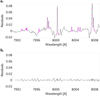 |
Fig. A.1. Residual spectrum between separated spectra of the two components and an observation with strong telluric lines. Panel a: residuals before correction. The dots represent the spline used to approximate the telluric lines. Panel b: residuals to the final corrected spectrum. |
Because the correction of the telluric lines in the wavelength range under consideration is crucial for the analysis, some details of this procedure are described here. A forthcoming paper by Sablowski et al. (2019) will discuss these disentangling problems in more detail.
The residual spectrum between the separated spectra and an observation is shown in Fig. A.1a. The identified tellurics are approximated by spline fits shown by dots. These splines were used to correct for the telluric lines in the observations. Special care was taken to identify the telluric lines such that no stellar signatures were affected. This was ensured by an iterative process: Only one line (we took the strongest) at a time was removed. The disentangling was performed again, and the next line with the highest contribution to the residuals was corrected. In this way, we corrected for all the telluric lines indicated by the dots in Fig. A.1a in all 12 observed spectra. The same residuals for the fully corrected observations after the final disentangling run is shown in Fig. A.1b.
Relative light ratio measurements for Capella.
Measurements of the light ratio for Capella are summarized in Table A.1 and plotted in Fig. A.2. The black solid line is the ratio r given by dividing two Planck relations r = aP(Teff,p)/P(Teff,s) with temperatures as given in Table 2. A multiplication factor a = 1.04 is needed to adapt to the data.
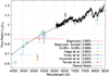 |
Fig. A.2. Visual presentation of the measurements of the light ratio for Capella (see also Table A.1). |
Appendix B: Spectrum of the secondary
To ensure that the disentangling is not affected by the tellurics or by the limited sampling of the orbit, further tests were performed. First, three spectra that show the smallest signal from tellurics were selected from the 12 spectra listed in Tabel 1. As pointed out by Sablowski & Weber (2017), at least 3 spectra are required because SVD has to be performed on an overdetermined system of equations, that is, for two components present in the spectra, at least three observations are required. Furthermore, these spectra should correspond to distinctive orbital phases. The separated spectra obtained from that data set are in excellent agreement with the spectra used for the synthesis (see Fig. B.1a). Second, to show that the orbital sampling by the observations is sufficient for the disentangling, 12 spectra were created by the use of synthesized spectra covering the same orbital phases as the observed spectra listed in Table 1. The excellent agreement between the templates (the synthesized spectra) and the separated spectra is shown in Fig. B.1b.
Line data for the synthesis of the secondary.
The weak feature around the 8004 Å lines can almost entirely be reproduced by the blend lines (Fe I 8002.6 Å, 8003.2 Å, Al I 8003.2 Å, and Ti I 8003.5 Å) and with a carbon abundance as derived for the primary. However, we show the separated spectrum together with a theoretical spectrum in Fig. B.1c. We used the parameters given in Table 2 and a macroturbulent velocity of 7.0 km s−1. The used line list is a combination of the list provided by Carlberg et al. (2012) and selected lines (with significant strengths) from VALD-3. The blue-side line to the strong Fe I 7998.944 Å could not be identified. It is too strong for a 12CN line (it would disagree with lines at 8004 Å). VALD-3 lists a central depth of the fitted Fe I 7998.944 of 0.534. There are only two lines listed in VALD-3 with significant depth: Fe I 7996.8156 Å with a depth of 0.026 and Ti I 7996.4350 Å with a depth of 0.072, but they are too weak to fit the observation. The NIST atomic line data base (Kramida et al. 2018) lists only one further and rather exotic posibility of an Th I line with unknown log gf value. A synthesis would lead to unrealistic abundance and high log gf value for that line. Furthermore, we plot the synthetic spectrum of the 13CN lines (blue line, abundance as derived for the primary).
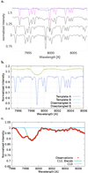 |
Fig. B.1. Panel a: three selected observations (each shifted on y by 0.2 for better visibility) with the weakest telluric feature (black) and the separated spectra (purple and blue) from these observations. The separated spectra are shifted in wavelength to match the topmost observation. The separated spectra are scaled such that the line strength matches the strengths in the observations. Panel b: synthetic spectra (used as templates to create an artifical binary data set) in comparison with the separated spectra (see text). Panel c: separated spectrum (red) of the G0III secondary of Capella with a synthetic spectrum (green). This was derived with the stellar parameters as listed in Table 2 and the line list given in Table B.1. It shows predominantly only the strong Fe I 7999 Å line. The blue line is a synthetic spectrum based on the 13CN lines as with an abundance as derived for the primary. |
All Tables
All Figures
|
Fig. 1. Twelve Capella spectra that were used for the disentanglement. The bottom spectrum is the first spectrum listed in Table 1. The others are shifted in intensity by +0.2 for better visibility. The spectra are shown in laboratory wavelength scale (prior to heliocentric correction), and some telluric features are marked with vertical red lines. |
| In the text | |
|
Fig. 2. Separated spectra of the G8III primary for the 8004 Å wavelength region of Capella. Light gray vertical lines define three continuum points, and the orange regions indicate the two fit regions for the spectrum synthesis. |
| In the text | |
|
Fig. 3. Synthesis for refining the values of the broadening mechanisms by a few isolated lines within the separated region. The final values are ξt = 1.39 km s−1, ζ = 6.0 km s−1, and v sin i = 3.8 km s−1. |
| In the text | |
|
Fig. 4. Panel a: result from the spectrum synthesis fitting with SME. The observations are shown as dots, and we plot the best fits as blue and green lines for the 12CN and 13CN line region, respectively. This suggests an isotope ratio of 17.8 ± 1.9. The synthetic spectra for ±3σ deviations are shown as orange and red lines, respectively. Panel b: spectrum synthesis with MOOG for consistency of the spectral fitting by SME. See text for the parameters of the underlying MARCS model. Panel c: observations minus synthesis (O-S) for the MOOG synthesis. Error bars corresponds to an S/N of 1000. |
| In the text | |
|
Fig. 5. rms between synthesized spectra from MOOG vs. CIR with the use of MARCS models (see text) with ξt = 1.0 km s−1and ξt = 2.0 km s−1, respectively. |
| In the text | |
|
Fig. A.1. Residual spectrum between separated spectra of the two components and an observation with strong telluric lines. Panel a: residuals before correction. The dots represent the spline used to approximate the telluric lines. Panel b: residuals to the final corrected spectrum. |
| In the text | |
|
Fig. A.2. Visual presentation of the measurements of the light ratio for Capella (see also Table A.1). |
| In the text | |
|
Fig. B.1. Panel a: three selected observations (each shifted on y by 0.2 for better visibility) with the weakest telluric feature (black) and the separated spectra (purple and blue) from these observations. The separated spectra are shifted in wavelength to match the topmost observation. The separated spectra are scaled such that the line strength matches the strengths in the observations. Panel b: synthetic spectra (used as templates to create an artifical binary data set) in comparison with the separated spectra (see text). Panel c: separated spectrum (red) of the G0III secondary of Capella with a synthetic spectrum (green). This was derived with the stellar parameters as listed in Table 2 and the line list given in Table B.1. It shows predominantly only the strong Fe I 7999 Å line. The blue line is a synthetic spectrum based on the 13CN lines as with an abundance as derived for the primary. |
| In the text | |
Current usage metrics show cumulative count of Article Views (full-text article views including HTML views, PDF and ePub downloads, according to the available data) and Abstracts Views on Vision4Press platform.
Data correspond to usage on the plateform after 2015. The current usage metrics is available 48-96 hours after online publication and is updated daily on week days.
Initial download of the metrics may take a while.