| Issue |
A&A
Volume 620, December 2018
|
|
|---|---|---|
| Article Number | A195 | |
| Number of page(s) | 15 | |
| Section | Stellar structure and evolution | |
| DOI | https://doi.org/10.1051/0004-6361/201834263 | |
| Published online | 18 December 2018 | |
Inner disk structure of the classical T Tauri star LkCa 15⋆
1
Departamento de Fisica – ICEx – UFMG, Av. Antônio Carlos 6627, 30270-901 Belo Horizonte, MG, Brazil
e-mail: This email address is being protected from spambots. You need JavaScript enabled to view it.
2
Université Grenoble Alpes, CNRS, IPAG, 38000 Grenoble, France
e-mail: This email address is being protected from spambots. You need JavaScript enabled to view it.
3
IRAP, Université de Toulouse, CNRS, UPS, CNES, 14 Avenue Edouard Belin, 31400 Toulouse, France
e-mail: This email address is being protected from spambots. You need JavaScript enabled to view it.
4
Crimean Astrophysical Observatory, Scientific Research Institute, 298409 Nauchny, Russia
5
ESO, Karl-Schwarzschild-Str. 2, 85748 Garching, Germany
6
NASA Ames Research Center, Moffett Field, CA 94035, USA
7
SUPA, School of Physics and Astronomy, Univ. of St Andrews, St Andrews, KY16 9SS, UK
8
Kavli Institute for Astronomy and Astrophysics, Peking University, Yi He Yuan Lu 5, Haidian Qu, Beijing 100871, PR China
9
CFHT Corporation, 65–1238, Mamalahoa Hwy, Kamuela, HI 96743, USA
10
Institute of Astronomy and Astrophysics, Academia Sinica, PO Box 23-141, 106 Taipei, Taiwan
Received:
17
September
2018
Accepted:
25
October
2018
Abstract
Context. Magnetospheric accretion has been thoroughly studied in young stellar systems with full non-evolved accretion disks, but it is poorly documented for transition disk objects with large inner cavities.
Aims. We aim at characterizing the star-disk interaction and the accretion process onto the central star of LkCa 15, a prototypical transition disk system with an inner dust cavity that is 50 au wide.
Methods. We obtained quasi-simultaneous photometric and spectropolarimetric observations of the system over several rotational periods. We analyzed the system light curve and associated color variations, as well as changes in spectral continuum and line profile to derive the properties of the accretion flow from the edge of the inner disk to the central star. We also derived magnetic field measurements at the stellar surface.
Results. We find that the system exhibits magnetic, photometric, and spectroscopic variability with a period of about 5.70 days. The light curve reveals a periodic dip, which suggests the presence of an inner disk warp that is located at the corotation radius at about 0.06 au from the star. Line profile variations and veiling variability are consistent with a magnetospheric accretion model where the funnel flows reach the star at high latitudes. This leads to the development of an accretion shock close to the magnetic poles. All diagnostics point to a highly inclined inner disk that interacts with the stellar magnetosphere.
Conclusions. The spectroscopic and photometric variability on a timescale of days to weeks of LkCa 15 is remarkably similar to that of AA Tau, the prototype of periodic dippers. We therefore suggest that the origin of the variability is a rotating disk warp that is located at the inner edge of a highly inclined disk close to the star. This contrasts with the moderate inclination of the outer transition disk seen on the large scale and thus provides evidence for a significant misalignment between the inner and outer disks of this planet-forming transition disk system.
Key words: accretion, accretion disks / stars: pre-main sequence / stars: individual: LkCa 15
Based on observations obtained at the Canada-France-Hawaii Telescope (CFHT) which is operated by the National Research Council of Canada, the Institut National des Sciences de l’Univers of the Centre National de la Recherche Scientifique of France, and the University of Hawaii.
© ESO 2018
1. Introduction
Classical T Tauri stars (CTTSs) are young (∼1−10 Myr), low-mass (M < 2 M⊙) stars surrounded by a circumstellar disk from which they accrete. Their magnetic fields are strong enough to truncate the inner disks and channel the accreting gas. These systems also produce outflows in the form of stellar and disk winds that may collimate in a jet (Bouvier et al. 2007b; Hartmann et al. 2016). At about the same ages, T Tauri stars that are no longer accreting are called weak-line T Tauri stars (WTTSs).
LkCa 15 is a K5, ∼1 M⊙ classical T Tauri star with an age of about 3–5 Myr (Simon et al. 2000), located at a distance of 159 ± 1 pc (Gaia Collaboration 2018) in the Taurus-Auriga star-forming region. It presents a transition disk, as defined by Strom et al. (1989). Its gas disk component, extending out to 900 au, was directly imaged through 12CO 2-1 emission with the IRAM Plateau de Bure interferometer (PdBI) by Piétu et al. (2007). The 50 au dust cavity in the disk was first spatially resolved by 1.4 mm and 2.8 mm PdBI observations (Piétu et al. 2006) and was later confirmed by dust continuum emission at 850 μm with Small Millimeter Array (SMA) observations (Andrews et al. 2011) and at 7 mm with the Very Large Array (VLA; Isella et al. 2014). Scattered light from small dust components was observed in the optical and infrared through imaging polarimetry with the Zurich Imaging Polarimeter of the Spectro-Polarimetric High-contrast Exoplanet REsearch (SPHERE/ZIMPOL) and the Infra-Red Dual Imaging and Spectrograph (IRDIS; Thalmann et al. 2015, 2016). The system is composed of a possibly warped inner disk, according to polarimetric differential imaging results obtained with the High-Contrast Coronographic Imager for Adaptive Optics (HiCIAO) of the Subaru telescope (Oh et al. 2016), a ∼50 au dust gap, and an outer disk (Thalmann et al. 2015). Modelling for the outer disk suggests inclinations of 44°–50° (Oh et al. 2016; Thalmann et al. 2014) with respect to our line of sight. Inside the dust cavity, gas was detected through CO 4.7 μm emission by Najita et al. (2003), revealing the presence of warm gas down to 0.083 ± 0.030 au (assuming i = 52°). At even smaller scales, the photometric and spectroscopic variability of LkCa 15 provides some insight into the interaction between the central star and the inner disk. Grankin et al. (2007) reported a six-year-long light curve for the system that exhibits a nearly constant brightness level interrupted by recurrent dimmings of up to one magnitude, with a periodicity of about six days (Artemenko et al. 2012). Such a light curve is typical of the so-called dippers (Cody et al. 2014) and is thought to result from the obscuration of the central star by rotating circumstellar dusty clumps in highly inclined systems (e.g., McGinnis et al. 2015). Whelan et al. (2015) further reported line profile variability in the optical and near-infrared spectra of the system, with the transient occurrence of inverse P Cygni profiles, that is, the appearance of redshifted absorption components up to velocities of 400 km s−1. These features are usually interpreted as the signature of accretion funnel flows along an inclined magnetosphere in young stellar systems (e.g., Hartmann et al. 1994, 2016). The photometric behavior and the spectral line profiles suggest that the system has an inner disk that interacts with the central star, seen at high inclination. LkCa 15 was previously classified by Espaillat et al. (2007) as a pre-transition disk, implying the presence of an inner disk, and Thalmann et al. (2016) reported shadows in the outer disk that would indicate some structure located close to the star. The high inclination of the inner disk suggested by the photometric and spectrocopic observations, however, is somewhat unexpected compared to the moderate inclination suggested by the modeling of high angular resolution imaging observations of the outer disk of LkCa 15.
These preliminary results provided the motivation for an in-depth study of the spectrophotometric variability of this prototypical transition disk system in Taurus. We therefore designed a campaign to obtain spectropolarimetric observations together with multi-color photometric observations on a timescale of weeks with the hope of clarifying how accretion proceeds onto the central star in a transition disk system with a large inner hole, thus attempting to relate the immediate circumstellar environment of the star to the large-scale properties of its circumstellar disk. In the following sections we detail the observations (Sect. 2), analyze the ground-based and K2 photometric data (Sect. 3), and discuss the spectroscopic results (Sect. 4). In Sect. 5 we give a global interpretation for the observed variability of LkCa 15, and we present our conclusions in Sect. 6.
2. Observations
BVRI photometric observations of the LkCa 15 system were obtained at the Crimean Astrophysical Observatory (CrAO) from November 13, 2015, to March 31, 2017, on the AZT-11 1.25 m telescope with a five-channel photometer or a CCD camera with the ProLine PL23042 detector. A nearby control star of similar brightness (TYC 1278-166-1) was used to estimate the photometric rms error in each filter, which amounts to 0.02, 0.014, 0.013, and 0.012 in the BVRI bands, respectively. A comparison star, HD 284589, was also observed in the BVRI filters with a five-channel photometer, thus providing the required calibration for the differential light curves derived from CCD photometry. Averaged extinction coefficients were assumed for the site. The brightness and colors of the comparison star in the Johnson system are 10.78 (V), 1.57 (B − V), 1.21 (V − RJ), and 2.03 (V − IJ). Unfortunately, only five measurements were obtained in the B band, and they are not considered further here. CCD images were obtained in VRI filters and were bias subtracted and flat-field calibrated following a standard procedure.
High-resolution spectroscopy was performed on the LkCa 15 system at the 3.6 m Canada-France-Hawaii Telescope (CFHT), using the Echelle SpectroPolarimetric Device for the Observation of Stars (ESPaDOnS; Donati 2003; Silvester et al. 2012). A first series of 14 optical spectra, ranging from 370 to 1050 nm, were obtained between November 18 and December 3, 2015 (the 2015B dataset), at a resolving power of about 68 000 and with a signal-to-noise ratio (S/N) of about 150 at 666 nm. A second series of 11 observations were obtained from December 13, 2016, to January 17, 2017 (the 2016B dataset) with the same setting. Observations were made using the spectropolarimetric mode, which provides simultaneous Stokes V (circularly polarized) and I (total intensity) spectra. Observations were reduced using the Libre-ESpRIT package (Donati et al. 1997). In this paper we mostly investigate the 2015B spectral variability of the LkCa 15 system based on the intensity spectra, while a detailed discussion of the polarized spectra is deferred to a companion paper (Donati et al. 2019).
3. Photometry
A V-band light curve of LkCa 15, shown in Fig. 1, was obtained at CrAO over two seasons. The system exhibits large V-band variability of up to 0.4 mag during the 2015/16 season and up to 1 mag during the 2016/17 season. Figure 1 suggests that the variability amplitude was smaller in 2015 than in 2016. However, the former epoch contains far fewer measurements than the second, and it is unclear whether deeper minima might have been missed. the better sampled 2015 ASAS-SN light curve shown in Fig. 2 has the same amplitude as the CrAO 2016 light curve, which suggests that the photometric behavior did not change drastically between the two epochs. Only some photometric measurements were obtained simultaneously with the 2015B spectroscopic observations, namely on November 17 and 20, 2015. Fortunately, the LkCa 15 photometric variability appears to be relatively stable over the years, as demonstrated by the V-band light curve obtained by Grankin et al. (2007) for this system over six seasons from 1992 to 1997. The average V-band magnitude and the variability amplitude we measure on the 2015–2017 light curve compare well with the values they report. Another similarity is the nearly constant maximum brightness level interrupted by deep minima that occur on a timescale of days. Even though the sampling of the CrAO light curve is not optimal, this type of light curve is strongly reminiscent of dippers (e.g., McGinnis et al. 2015; Rodriguez et al. 2017; Bodman et al. 2017).
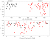 |
Fig. 1. Upper panel: V-band light curve of LkCa 15 obtained at CrAO over seasons 2015/16 (red) and 2016/17 (black). Lower panel: CrAO light curve folded in phase with a period of 5.70 days and JD0 = 2457343.8. The dates of spectroscopic observations of the 2015B dataset are indicated by black arrows. |
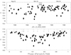 |
Fig. 2. Upper panel: V-band light curve obtained from ASAS-SN for the season 2015/16. Lower panel: ASAS-SN light curve folded in phase with a period of 5.70 days and JD0 = 2457343.8. The dates of spectroscopic observations are indicated by black arrows. |
We searched for periodicities in the light curve in the full dataset and independently for each season. A CLEAN periodogram analysis (Roberts et al. 1987) and a string-length analysis (Dworetsky 1983) both resulted in periods being detected in the full dataset as well as in each season, ranging from 5.62 to 5.70 days. This is slightly shorter than the periods of 5.86–6.03 days that were previously reported for the system by Bouvier et al. (1993) and Artemenko et al. (2012). Figure 1 shows the V-band light curve phased with a period of 5.70 days. It concentrates most of the photometric minima around phases 0.4–0.6, but with a significant photometric scatter at all phases, which is typical of dippers. Additional photometry for the 2015/2016 season is available from ASAS-SN (Shappee et al. 2014; Kochanek et al. 2017), and the corresponding light curve is shown in Fig. 2. A periodogram analysis yields a period of 5.70 ± 0.05 days, consistent with that derived from the CrAO dataset. We used this as the stellar rotation period here. The corresponding phase diagram is shown in the lower panel of Fig. 2.
Finally, the Kepler K2 satellite monitored LkCa 15 in a broad bandpass ranging from 420 to 900 nm during Campaign F13 from March 8 to May 27, 2017. While these observations occurred more than a year after the spectral series discussed in this paper (2015B dataset), the unsurpassed quality of the K2 light curve provides a much deeper insight into the photometric variability of the system. The light curve, encompassing 80 days uninterrupted, is shown in Fig. 3 and clearly confirms that LkCa 15 is a dipper: a nearly constant flux level is periodically interrupted by brightness dips lasting for a few days with an amplitude of up to one magnitude. A period analysis reveals a clear signal at 5.78 days, present over the 13 rotational cycles the K2 light curve samples. The phased light curve is shown in the lower panel of Fig. 3. The photometric minima often last for a significant fraction of the period, which suggests that an extended inner disk warp produces the dips (Romanova et al. 2013; Romanova & Owocki 2015). While periodic, the dips vary in shape, and their width, depth, and phase evolve from one cycle to the next. This is indicative of a dynamic interaction between the inner disk and the stellar magnetosphere. This behavior is quite reminiscent of that of the prototype of the dipper class, AA Tau (e.g., Bouvier et al. 2007a).
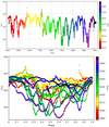 |
Fig. 3. Upper panel: Kepler K2 light curve obtained for LkCa 15 from March 7 to May 28, 2017. The light-curve morphology is clearly that of a dipper. Lower panel: K2 light curve folded in phase with a period of 5.78 days. The color code is the same in both panels and reflects the Julian Date of observations. Two flare-like events are visible in the light curve (t = 7838 and 7851). |
CrAO multi-band photometry provides information on the color changes associated with the flux variations. Over the two observing seasons, the system exhibited color variations amounting to a few tenths of a magnitude, as shown in Fig. 4. The system becomes redder when fainter, with little scatter around a mean color slope of 0.19 in the (V, V − RJ) color–magnitude diagram and 0.33 in the (V, V − IJ) diagram. These slopes are different from those expected for an interstellar medium (ISM)-like reddening vector, which would amount to 0.27 and 0.49 in the (V, V − RJ) and (V, V − IJ) diagrams, respectively. The (V − RJ) color range and color slope are similar to the values reported by Grankin et al. (2007) from the long-term photometric monitoring of the system.
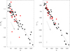 |
Fig. 4. (V − RJ) vs. V (left panel) and (V − IJ) vs. V (right panel) color–magnitude variations of the system during the 2015/16 (red) and 2016/17 (black) season from CrAO photometry. The straight line in each panel is a linear regression fit to the color slope. Arrows indicate ISM-like extinction vectors. Photometric error bars are indicated in the bottom left corner of each panel. |
4. Spectroscopy
4.1. Veiling and radial velocities
Classical T Tauri stars (CTTSs) present hot spots at the stellar surface that emit an extra continuum, which is added to the stellar continuum and veils the photospheric lines, decreasing their depths. Veiling is measured as the hot-spot continuum flux divided by the stellar continuum flux at a given wavelength. Therefore, a veiling of 1 corresponds to an equal contribution from the hot spot and the star to the observed continuum. CTTSs also have cold spots that are due to magnetic field emergence at the stellar surface. Hot and cold spots represent regions at different temperatures than the stellar photosphere and can cause significant distortions in the photospheric line profiles that mimic radial velocity variations.
Veiling and photospheric radial velocities were calculated from the continuum-normalized spectra of LkCa 15 in five spectral regions of about 100 Å wide, close to 4800 Å, 5300 Å, 5600 Å, 6000 Å, and 6300 Å. We used as a standard the weak-lined T Tauri star V819 Tau (K4, Teff = 4250 ± 50 K) that was observed with ESPaDOnS (CFHT), with the same settings as LkCa 15, as part of the MaTYSSE program (Donati et al. 2015). V819 Tau rotates slowly (ν sin i⋆ = 9.5 ± 0.5 km s−1) and matches the LkCa 15 photospheric lines well. The standard spectrum was rotationally broadened, veiled, and cross-correlated with each spectrum of LkCa 15 until a best match was found. This procedure allows the simultaneous determination of veiling and radial velocities.
We searched for periodical variations in the veiling and radial velocities using the Scargle periodogram as modified by Horne & Baliunas (1986). Errors were estimated as the standard deviation of a Gaussian fitted to the main peak of the periodogram power spectrum. The veiling and radial velocity present periodicities at 5.55 ± 0.71 days and 5.55 ± 0.77 days, respectively, which agree with the photometric period of 5.70 ± 0.05 days within the errors. The veiling and the radial velocity periods should correspond to the stellar rotation period, since hot and cold spots are located at the stellar surface. The agreement between the veiling and radial velocity period and the photometric period supports the hypothesis that the inner disk warp is located close to the disk corotation radius. In Fig. 5 we show the mean veiling and radial velocity values obtained at each phase and the corresponding standard deviations. The standard deviations were computed with the veiling and radial velocity values calculated at each observing date in the five different spectral regions we analyzed. The phases in Fig. 5 were calculated with a photometric period of 5.70 days and an arbitrary JD0 = 2457343.8, chosen to ensure that the photometric minimum of the ASAS-SN light curve was around phase 0.5. The maximum veiling is coincident with the photometric minimum, which indicates that the accretion spot is aligned with the inner disk warp.
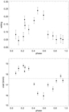 |
Fig. 5. Veiling (top panel) and radial velocities (bottom panel) of LkCa 15 in phase with the 5.7-day ASAS-SN photometric period and JD0 = 2457343.8. The dashed line corresponds to the mean νrad = 17.83 ± 0.86 km s−1. |
We fit synthetic spectra to the observations in the spectral region that extends from 6060 to 6155 Å using a version of the ZEEMAN spectrum synthesis code (Landstreet 1988; Wade et al. 2001; Folsom et al. 2016) that allows for an additional continuum flux to be fit together with the stellar spectrum. This spectral region was chosen because it presents many atomic lines with few blends. We made some initial fits, and it became clear that the surface gravity (g) was poorly determined. We therefore estimated log g using the stellar mass value determined by Simon et al. (2000) from the circumstellar disk rotation curve, and the stellar radius obtained from the stellar luminosity calculated by Herczeg & Hillenbrand (2014), after scaling the values to take into account the LkCa 15 distance of 159 ± 1 pc measured by the Gaia satellite (Gaia Collaboration 2018). With the scaled values of M⋆ = 1.10 ± 0.03 M⊙ and L⋆ = 0.80 ± 0.15 L⊙, and using Teff in the range of 4350 K–4500 K, which corresponded to our best initial fits, we obtained log g = 4.10 ± 0.10. Keeping log g fixed at 4.0, 4.1, or 4.2, we again fit the observed spectra with Teff, the projected rotational velocity (ν sin i⋆), the radial velocity, and the veiling as free parameters. We then noted that two of the spectra, from JD = 7350.8645 to 7352.8529, converged to much higher values of ν sin i⋆ than the others. At these dates, the Moon was very close to the star, and we decided to forego using these two spectra} in the determination of stellar parameters to avoid contamination. We applied our fitting procedure to the 12 remaining spectra with the fixed log g values and obtained Teff = 4492 ± 50 K and ν sin i⋆ = 13.82 ± 0.50 km s−1, where the values correspond to the average and the errors to the standard deviation of the best-fit results of our grid. With our effective temperature and the stellar luminosity of 0.80 ± 0.15 L⊙, we calculated a stellar radius of 1.49 ± 0.15 R⊙. According to the Siess et al. (2000) and Marques et al. (2013) evolutionary models, for a mass estimate in the range between 1.10 M⊙ (Simon et al. 2000) and 1.25 M⊙ (Donati et al. 2019), LkCa 15 is no longer fully convective and has already developed a radiative core.
The mean ν sin i⋆ = 13.82 ± 0.50 km s−1 obtained during the spectral fit together with the adopted photometric period of 5.70 ± 0.05 days (see Sect. 3) and the stellar radius of 1.49 ± 0.15 R⊙ yield sin i⋆ larger than 0.90, within the error bars of the measured values. This corresponds to stellar inclinations i⋆ > 65°, which are higher than the outer disk inclination of 44°–50° measured from optical and infrared polarimetric imaging (Thalmann et al. 2015, 2016; Oh et al. 2016). This suggests a misalignment between the inner and outer disks.
4.2. Photospheric LSD profiles
We calculated least-squares deconvolution (LSD) photospheric profiles (Donati et al. 1997) using a line mask computed from a Vienna Atomic Line Database (VALD; Piskunov et al. 1995) line list with Teff = 4500 K and log g = 4.0. Emission, telluric, and broad lines were excluded from the mask, since they do not represent the photospheric weak-line profile. We also removed all the lines before 5000 Å because the S/N in the blue of our spectra was weak. The photospheric LSD profiles were normalized with a mean wavelength, Doppler width, line depth, and Landé factor of 670 nm, 1.8 km s−1, 0.55, and 1.2, following Donati et al. (2014). We corrected the LSD profiles for veiling, using the mean veiling values displayed in Fig. 5. The intensity of each point of the normalized and veiled spectrum (I) is related to the mean veiling value (ν) and the non-veiled line intensity (I0) by  , which allows the recovery of I0, knowing I and ν. The Stokes I LSD profiles show a periodic variability at 5.56 ± 0.74 days, as we show in Fig. 9. Stellar radial velocities, computed from the first moment of the Stokes I LSD profiles, also presented a periodicity at 5.62 ± 0.75 days. These period values agree with the photometric and veiling periodicities.
The longitudinal component of the magnetic field can be computed from the first moment of the Stokes V LSD profiles (see Donati et al. 1997). The longitudinal magnetic field values computed with our veiling-corrected LSD profiles are shown in Fig. 6. They vary from −29 G to +87 G and show a periodicity at 5.76 ± 0.74 days, corresponding to the mean rotation period of the star, and in agreement with the veiling, radial velocities, and the photometric periods.
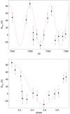 |
Fig. 6. Longitudinal component of the magnetic field of LkCa 15 from LSD profiles as a function of time (top panel) and in phase (bottom panel) with the 5.7-day ASAS-SN photometric period and JD0 = 2457343.8. A sine wave with the 5.7-day period is overplotted. |
4.3. Circumstellar line profiles
LkCa 15 displayed emission line profiles that were strongly variable during our observations. The high resolution of the ESPaDOnS spectra enabled us to identify several emission and absorption components and analyze their variability. We also calculated 2D Scargle periodograms, as modified by Horne & Baliunas (1986), on the line profile intensities. Errors were estimated as the mean standard deviation of a Gaussian fit to the main peak of the periodogram power spectrum over the velocity range of the period detection. The results are displayed in Fig. 9. Our spectroscopic data in 2015A span 15 days, therefore we only considered period detections shorter than 7.5 days.
HeI 5876 Å presents one of the simplest emission line profiles in our observations, showing only a narrow emission component (FWHM < 60 km s−1, according to Beristain et al. 2001) that periodically varies in intensity, as shown in Figs. 7–9. The strongest emissions are seen close to phase 0.5, when the veiling is maximum and we expect the accretion spot to be in our line of sight (Fig. 7, right). This is in agreement with a scenario where the HeI 5876 Å line is mostly formed in the postshock region, at the base of the accretion column (Beristain et al. 2001). The strong modulation of the HeI 5876 Å emission, which almost completely disappears at some phases, suggests a high inclination of the inner disk, given the relatively low obliquity (20−25°) of the stellar magnetic field with respect to the stellar rotation axis (see Sect. 5 and Donati et al. 2019). The HeI 5876 Å line shows a well-defined periodic signal at 5.63 ± 0.66 days in all velocity bins. The accretion spot period should correspond to the stellar rotation period, and it indeed agrees with the period calculated from the variation of the longitudinal magnetic field of the star. It also agrees within the errors with the photometric period and supports the assumption that the inner disk warp, mapped by the photometric variations, is located near the disk corotation radius.
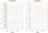 |
Fig. 7. Observed HeI 5876 Å profiles in time (left panel) and in phase (right panel) with the 5.7-day ASAS-SN photometric period and JD0 = 2457343.8. The red lines represent the continuum level. |
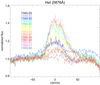 |
Fig. 8. Observed HeI 5876 Å profiles overplotted. The observation dates are shown with the same color code as the profiles. |
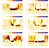 |
Fig. 9. HeI 5876 Å NaD, CaII 8542 Å Hβ, Hα and LSD line periodograms. The top color bars represent the periodogram power, varying from zero (white) to the maximum power (black). The black horizontal lines correspond to the highest power period of each line, as discussed in the text. |
The NaD doublet is mostly photospheric and in absorption, but a strong variability is present in its redshifted wing, hinting at a possible circumstellar contribution from high-velocity free-falling gas to this part of the profile, as shown in Fig. 10. To enhance the redshifted variability, we subtracted the mean observed profile from the observations, and we show in Fig. 11 that it extends up to 350 km s−1. These redshifted absorptions are periodic at 5.41 ± 0.64 days (Fig. 9), in agreement with an origin close to the stellar surface in the high-velocity gas that falls freely toward the star.
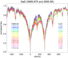 |
Fig. 10. Observed NaD doublet profiles overplotted. The observation dates (left) and the phases (right) are shown with the same color code as the profiles. |
 |
Fig. 11. Mean profile subtracted from the NaD profiles, in time (left panel) and in phase (right panel) with the 5.7-day ASAS-SN photometric period and JD0 = 2457343.8. The red lines represent the continuum level. |
The CaII 8542 Å line is part of the CaII infrared triplet. The original spectrum shows a narrow emission of chromospheric and postshock origin inside a photospheric absorption profile. To evaluate only the circumstellar contribution to the line profiles, we calculated residual spectra by subtracting the rotationally broadened and veiled spectrum of V819 Tau from the observed spectra. The residual line profile (Figs. 12 and 13) is composed of a narrow emission, a broad emission that can be either blueshifted or redshifted, and a redshifted absorption component that preferentially appears around phase 0.5, when the main accretion column is expected to be in our line of sight. The redshifted absorption component is indicative of accretion, and is thought to originate in the accretion funnel, when photons from the accretion spot are absorbed by gas in the funnel at high velocity, moving away from us. This part of the profile presents a periodicity at 5.56 ± 0.65 days (Fig. 9), in agreement with the HeI 5876 Å and the photometric period. The narrow emission, however, apparently shows a slightly longer variability at 6.7 ± 1.0 days. To investigate the different periodicity presented by the narrow emission, we decomposed the CaII 8542 Å profiles by fitting 1, 2, or 3 Gaussians, depending on the number of components present. The decomposition allows the individual analysis of each component variability. After separating the narrow emission and the broad component emission, we searched for periodicities in the component intensities, equivalent widths (EW), and radial velocities. The narrow emission intensity and EW present periods of 5.76 ± 0.80 days and 5.83 ± 0.80 days, respectively, but no significant period was found with the radial velocity variations. The broad emission component shows strong variability, both in radial velocity and intensity, but we were unable to detect a significant period. Only ten observations present this component, which can be either blueshifted or redshifted. The period at 6.7 ± 1.0 days detected in the 2D periodogram near the line center therefore probably comes from the mixed variability of the superposed narrow and broad emissions.
 |
Fig. 12. Residual CaII 8542 Å profiles in time (left panel) and in phase (right panel) with the 5.7-day ASAS-SN photometric period and JD0 = 2457343.8. The red lines represent the continuum level. |
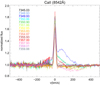 |
Fig. 13. Residual CaII 8542 Å profiles overplotted. The observation dates are shown with the same color code as the profiles. |
The CaII 8542 Å line presents a clear signal in Stokes V, which is as broad as the narrow emission component present in the Stokes I data. We subtracted from the residual CaII 8542 Å Stokes I profiles a Gaussian fit to the broad emission component present in some spectra, and we calculated the longitudinal magnetic field as the first moment of the Stokes V data. The results are shown in Fig. 14. The longitudinal magnetic field in the region of CaII 8542 Å formation varies in polarity and intensity from −118 G to +660 G, and is stronger near phase 0.5, in agreement with the maximum veiling, which indicates that this is when the accretion spot faces us. The variation is periodical at 5.41 ± 0.74 days, which agrees with the stellar rotation period within the errors. This result strongly suggests that part of the narrow CaII emission is produced in the postshock region.
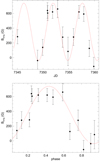 |
Fig. 14. Longitudinal component of the magnetic field of LkCa 15 from CaII 8542 Å profiles as a function of time (top panel) and in phase (bottom panel) with the 5.7-day ASAS-SN photometric period and JD0 = 2457343.8. A sine wave at the 5.7-day period is overplotted. |
The Hβ spectral region presents several photospheric absorption lines that are superposed on the Hβ emission. To remove the photospheric lines, we again calculated residual profiles by subtracting the rotationally broadened and veiled spectrum of V819 Tau. The resulting spectra are shown in Figs. 15 and 16. The residual Hβ line profile is complex and presents an emission with several absorption components of non-photospheric origin. We can identify a blueshifted absorption component near 50 km s−1, a low-velocity redshifted absorption component, and at some phases, a high-velocity redshifted absorption component. The latter is more visible near phase 0.5, but cannot be discarded at other phases. The red wing varies with a period of 5.56 ± 0.75 days and the line center at 5.85 ± 0.76 days (Fig. 9), both agreeing with the variability of the HeI 5876 Å line, the redshifted wing of CaII 8542 Å, and with the photometric period, hinting at an origin close to the stellar surface. The blue wing of the profile shows a more complex variability without a significant periodicity and may originate in various regions, such as the accretion funnel and a wind, that do not necessarily vary at the same period.
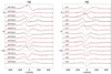 |
Fig. 15. Residual Hβ profiles in time (left panel) and in phase (right panel) with the 5.7-day ASAS-SN photometric period and JD0 = 2457343.8. The red lines represent the continuum level. |
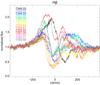 |
Fig. 16. Residual Hβ profiles overplotted. The observation dates are shown with the same color code as the profiles. |
The Hα emission line, like Hβ, presents a rather complex and variable profile, as we show in Figs. 17 and 18. A strong emission, a blueshifted absorption, and two redshifted absorption components can be clearly distinguished. One component lies close to line center and another, which is only present in a few spectra, is present at high velocity. In the Balmer series this is the line with the highest transition probability, and it is expected to form throughout the circumstellar environment of a CTTS: in the disk wind, the accretion funnel, the accretion spot, and stellar winds. Its variability can therefore be influenced by variations in all the circumstellar components, and it is not a surprise that most of the line does not present a single and highly significant period (Fig. 9). The only exception is the region near the line center, which shows a periodicity at 5.78 ± 0.68 days, like the same region of Hβ.
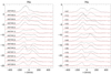 |
Fig. 17. Hα observed profiles in time (left panel) and in phase (right panel) with the 5.7-day ASAS-SN photometric period and JD0 = 2457343.8. The red lines represent the continuum level. |
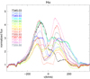 |
Fig. 18. Observed Hα profiles overplotted. The observation dates are shown with the same color code as the profiles. |
Although complex, the different components of the Hα profile are clearly distinguishable, which allowed us to decompose the profiles with Gaussians in order to measure their parameters. The decomposition is shown in Appendix A. The star-disk interaction is expected to be very dynamic, as shown by magnetohydrodynamics (MHD) simulations (Zanni & Ferreira 2013; Romanova et al. 2009; Kurosawa & Romanova 2012). The stellar magnetic field may interact with the inner disk at a range of radii, and as a result of differential rotation between the star and the disk, as the system rotates, the magnetic field lines inflate, twist, reconnect, and the cycle starts again. To probe the inflation of the magnetic field lines, we can analyze the radial velocity of the Hα absorption components, measured as the central velocity of the corresponding Gaussian components. The redshifted component is thought to come from the absorption of photons by the gas in the accretion column, and the blueshifted component is expected to trace the inner disk wind. As depicted in Fig. 19 of Bouvier et al. (2003), when the field lines inflate, the radial velocities of the redshifted and blueshifted components vary in opposite directions. This behavior was seen in two different observing campaigns of AA Tau (see Fig. 11 of Bouvier et al. 2007a), and it is clearly seen in our two observing seasons of LkCa 15 (Fig. 19).
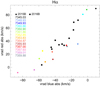 |
Fig. 19. Hα blueshifted and redshifted radial velocity variability. Filled circles represent the 2015B data and filled squares the 2016B data. The observation dates of the 2015B run we analyzed here are shown with the same color code as the corresponding points. |
4.4. Correlation matrices
Correlation matrices compare two sets of spectral lines that are observed simultaneously and show how correlated their variabilities are across the line profiles. A strong correlation among emission components, for example, indicates a common origin of the components. Correlation matrices can be calculated with datasets of the same line (autocorrelation), or different lines.
The HeI 5876 Å line consists of a single narrow component that varies at the stellar rotation period. Its autocorrelation matrix shows that the narrow component is coherent with a formation in a single region, as the entire profile is well correlated (Fig. 20, top left).
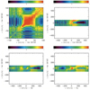 |
Fig. 20. HeI 5876 Å autocorrelation matrix (top left panel), CaII 8542 Å vs. HeI 5876 Å correlation matrix (top right panel), Hβ vs. HeI 5876 Å correlation matrix (bottom left panel), and Hα vs. HeI 5876 Å correlation matrix (bottom right panel). The top color bars represent the linear correlation coefficient, which varies from −1 (black), corresponding to anticorrelated regions, to +1 (red), corresponding to correlated regions. |
A comparison of the HeI 5876 Å line variations with the line profile variations of other emission lines can show which parts of the other lines are formed in about the same region as the HeI 5876 Å line.
The HeI 5876 Å line and the CaII 8542 Å narrow chromospheric emission present a good correlation (Fig. 20 top right), which indicates that both components are related to the accretion shock region. We also see a strong anticorrelation between the HeI 5876 Å line and the CaII 8542 Å or the Hβ high-velocity (ν > 150 km s−1) redshifted wings (Fig. 20 top right and bottom left). Since these parts of the CaII 8542 Å and Hβ profiles are dominated by the periodic appearance of a redshifted absorption component, the anticorrelation indicates that when the HeI profile is stronger, the redshifted component decreases (becomes deeper). This strongly relates the redshifted absorption component to the appearance of the accretion spot, as expected from magnetospheric accretion models.
The correlation matrix of Hα versus HeI reflects the complexity of Hα (Fig. 20 bottom right). Slightly redshifted from the Hα line center, we see a good correlation with the HeI line profile. This is a highly variable region in Hα and a substantial part of it is apparently related to the accretion flow close to the star. The Hα high-velocity blue wing, which does not present a strong variability, shows some anticorrelation with the HeI line that is difficult to interpret, since no clear component is associated with this part of the Hα line.
The CaII 8542 Å autocorrelation matrix shows that the red high-velocity wing of the profile correlates well with itself, but different parts of the line are not strongly correlated with each other (Fig. 21 top left). This indicates a formation in different regions. The Hβ autocorrelation matrix shows that the red high-velocity wing of the profile correlates well with itself, but different parts of the line are not strongly correlated with each other (Fig. 21 top right).
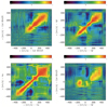 |
Fig. 21. CaII 8542 Å, Hβ and Hα autocorrelation matrices (top left, right, and bottom left panels), and Hβ vs. CaII 8542 Å correlation matrix (bottom right panel). The top color bars represent the linear correlation coefficient, which varies from −1 (black), corresponding to anticorrelated regions, to +1 (red), corresponding to correlated regions. |
The Hα autocorrelation matrix shows that the red high-velocity wing of the profile correlates well with itself, as in Hβ. We also clearly see that the line center is anticorrelated with the high-velocity blue wing, which is difficult to interpret (Fig. 21 bottom left).
The correlation matrix of Hβ versus CaII shows that the high-velocity red wings of both lines correlate well, as expected, since they are dominated by variations that are due to the redshifted absorption component (Fig. 21 bottom right). The CaII chromospheric emission and the blue wing of CaII show some correlation with the blueshifted Hβ emission. Finally, a strong anticorrelation is seen between the Hβ low-velocity and highly variable redshifted region and the CaII high-velocity component. This may indicate that this Hβ region originates preferentially close to the accretion spot.
5. Discussion
A consistent picture seems to emerge from the combined spectroscopic and photometric variability of the LkCa 15 system, as most of the observed continuum and spectral line variability can be understood in the framework of a magnetic interaction between an inclined inner disk with respect to our line of sight and the stellar magnetosphere. In the prototypical case AA Tau (e.g., Bouvier et al. 1999, 2003) and, more generally, in most periodic dippers (e.g., McGinnis et al. 2015; Rodriguez et al. 2017; Bodman et al. 2017), recurrent luminosity dimmings of up to one magnitude or more are interpreted as resulting from the occultation of the central star by a rotating inner disk warp located close to the corotation radius. The warp itself stems from the inclination of the large-scale stellar magnetosphere onto the stellar rotational axis: the magnetic obliquity forces the accreted material out of the disk midplane, thus creating a dusty, azimuthally extended inner disk warp (Romanova et al. 2013; Romanova & Owocki 2015). As the warp rotates at a Keplerian rate, it occults the central star periodically. The light curve and color variations of LkCa15 are fully consistent with this interpretation: the luminosity period dips (P = 5.70 days), their depth of up to one magnitude in the V band, the reddening of the system when fainter, and the changing shape of the eclipses from one cycle to the next are all characteristics of periodic dippers (e.g., Bouvier et al. 2007a; Alencar et al. 2010; Cody et al. 2014; McGinnis et al. 2015; Rodriguez et al. 2017; Bodman et al. 2017). For a stellar mass of 1.10 ±0.03 M⊙, and assuming Keplerian rotation for the inner disk, the occultation period of 5.70 ± 0.05 days would locate the inner disk warp at a distance of 9.3 ± 0.1 R⋆ = 0.064 ± 0.001 au from the central star.
We can compare the warp location with the magnetospheric radius that is due to a dipolar magnetic field as derived by Bessolaz et al. (2008),  , where ms ∼ 1 is the sonic Mach number measured at the disk midplane and B⋆, Ṁacc, M⋆ and R⋆ are in units of 140 G (at the stellar equator), 10−8 M⊙ yr−1, 0.8 M⊙, and 2 R⊙, respectively. We therefore need to estimate the stellar dipole component and the mass accretion rate during our observations. Our ZDI analysis of the 2015B data, which includes the LSD and CaII spectropolarimetric data, indicates that the dipole component of the magnetic field is of about 1.35 kG and tilted by ∼20° with respect to the stellar rotation axis (Donati et al. 2019). To calculate the mass accretion rate, we selected spectra outside the eclipses (rotational phases earlier than 0.2 or later than 0.8), and assumed V = 11.8 mag and (V − R)J = 1.1 at the time of the spectroscopic observations, which corresponds to the brightest state of LkCa 15 (see Figs. 1, 2 and 4). Using the expressions from Fernie (1983), we obtained (V – R)C = 0.78 and RC = 11.02. We measured the Hα equivalent widths in the five selected spectra and calculated the Hα flux (Table 1) with the out-of-eclipse value of RC. Adopting a distance to LkCa 15 of 159 ± 1 pc (Gaia Collaboration 2018), and the empirical relation obtained by Fang et al. (2009) between accretion and Hα line luminosity, we calculated the accretion luminosity. Mass accretion rates were derived from the relation
  (Hartmann et al. 1998), with the typical value of Rin = 5R⋆ that is commonly used in the literature. We obtained Ṁacc = (7.4 ± 2.8) × 10−10 M⊙ yr−1, which corresponds to the mean and standard deviation of our values presented in Table 1. Changing Rin from 5 to 10 R⋆ introduces a variation of ±1 × 10⁻¹⁰ M⊙ yr−1 in our mass accretion rate values, which is smaller than the standard deviation of the mass accretion rate from our five out-of-eclipse measurements. The dipole component of the magnetic field, together with the mass accretion rate, the stellar mass (1.10 ±0. 03 M⊙), and stellar radius (1.49 ± 0.15 R⊙), yield a magnetospheric radius of rm = 8.0 ± 1.4 R⋆ = 0.055 ± 0.015 au, which is consistent within the error bars with the corotation radius at 0.064 ± 0.001 au.
When we assume a sublimation temperature of 1500 K, the minimum dust sublimation radius is located at rsub = 4.48 ± 0.10 R⋆ = 0.031 ± 0.001 au (Eq. (1) with QR = 1 from Monnier & Millan-Gabet 2002), and consequently at rm = (8.0 ± 1.4) R⋆, there is dust left to form a warp. At the corotation radius, rcor = (9.3 ± 0.1) R⋆, dust would be present and the interaction of the stellar magnetic field and the inner disk could explain the presence of a warp there.
Accretion parameters of LkCa 15 calculated from the Hα line flux of out-of-eclipse observations.
We can also estimate the magnetospheric radius from the free-fall velocity (νff) of the accreting gas. The redshifted absorption components that are often observed at high velocities in NaD, CaII, and Hβ, extending up to 350 km s−1, correspond to the projected velocity of the accreting gas that in a simple dipolar case is νred = νff cos im, where im is the inclination of the magnetosphere with respect to our line of sight. We can then write
![Mathematical equation: $ \begin{equation} {\it \nu}_{\rm ff}=\frac{{\it \nu}_{\rm red}}{\cos(i_{\rm m})}=\left[\frac{2GM_{\star}}{R_{\star}}\left(1-\frac{R_{\star}}{r_{\rm m}}\right)\right]^{1/2} , \end{equation} $](/articles/aa/full_html/2018/12/aa34263-18/aa34263-18-eq4.gif) (1)
(1)
with im = i⋆ − β, where i⋆ is the inclination of the stellar axis onto the line of sight, and β represents the magnetic obliquity, that is, the angle between the magnetic and stellar axes. If the accretion spot is on the order of a few percent of the stellar photosphere, which is commonly the case in CTTSs, we can estimate the obliquity of the magnetic field from the radial velocity amplitude of the HeI 5876 Å line as Δνrad = 2ν sin i⋆ cos(π/2 − β) (Bouvier et al. 2007a). We fit the HeI 5876 Å emission line with a single Gaussian and measured Δ νrad = 11.6±1.0 km s−1. With ν sin i⋆ = 13.82±0.50 km s−1, we obtain β = 25°±5°, which is consistent with our value of β ∼ 20° calculated with ZDI (Donati et al. 2019). With β = 25° = i⋆ − im, i⋆ > 65°, R⋆ = 1.49 ± 0.15 R⊙, M⋆ = 1.10 ± 0.03 M⊙ and νred = 350 km s−1, we obtain from Eq. (1), rm > 0.014 au for i⋆ = 65°, and rm > 0.026 au for i⋆ = 75°, which are compatible with the warp location, given our errors.
When the dominant component of the stellar magnetosphere on a scale of a few stellar radii is a tilted dipole, the free-falling accretion funnel flow reaches the stellar surface at high latitudes, close to the magnetic poles. A strong shock forms, which yields continuum excess flux from X-ray to optical wavelengths, and produces line emission, in particular, the narrow component of the HeI 5876 Å feature, which is thought to arise in the postshock region (e.g., Beristain et al. 2001). Since the accretion spot rotates with the star, its visibility is modulated at the stellar rotation period, as should the veiling and line profile variations. This is observed in dippers, as well as in spotted, lower inclination systems, where spectroscopic observations have been conducted simultaneously with photometric observations (e.g., Bouvier et al. 2007a; Alencar et al. 2012; Fonseca et al. 2014; Sousa et al. 2016). This is precisely what we observe here in the LkCa 15 system: the veiling variations are periodic (P = 5.6 days), and reach a maximum at the rotational phase corresponding to the maximum longitudinal magnetic field measured in the CaII 8542 Å line profile, which is thought to form at least partly close to the accretion shock. The intensity of the HeI 5876 Å line profile also varies periodically (P = 5.6 days), being maximum at the phase of maximum veiling, as expected from the modulation of the accretion shock visibility. Like in AA Tau, the magnetospheric radius (0.055 ± 0.015 au) and the corotation radius (0.064 ± 0.001 au) are coincident within the errors. They are also consistent with the innermost CO emission radius (0.083 ± 0.030 au) measured by Najita et al. (2003). Moreover, the sublimation radius at (0.031 ± 0.001 au) indicates that dust can be present at the magnetospheric radius and fill an inner disk warp that is thought to be created by the dynamical interaction of an inclined stellar magnetosphere and the inner disk near corotation. All these features provide a direct measurement of the stellar rotation period, which agrees with the photometric period due to the inner disk warp, which must thus be located close to the corotation radius. Additional support for the magnetospheric accretion scenario to explain the observed variability of the LkCa 15 system comes from the appearance of high-velocity redshifted absorptions occurring in the profiles of the Balmer, NaD I, and CaII 8542 Å lines at phases ranging from 0.3 to 0.7, that is, corresponding to maximum accretion shock visibility. Redshifted absorptions occur when the colder gas in the upper part of the accretion flow absorbs the photons originating from the hotter gas located deeper down in the accretion column. The simultaneous occurrence of stellar occultations, redshifted absorption, and continuum excess confirms that the disk warp, the accreting gas, and the accretion shock are located at the same azimuth from the disk inner edge to the stellar surface, and thus are physically connected.
However, the magnetospheric accretion model does not straightforwardly account for other aspects of the spectral variability of the system reported here. For instance, neither the strong redshifted emission feature observed in the CaII 8542 Å line profile at phase 0.07 nor the anticorrelation of intensity variations between the HeI 5876 Å line and the extreme blue wing of the Hα line, possibly related to a fast wind, are easily understood. Moreover, the nearly opposite polarities measured in the longitudinal component of the magnetic field for the photospheric and CaII lines suggest a complex, multipolar field close to the stellar surface, even though the dipole may still dominate at the corotation radius. This would not be surprising for LkCa 15, whose partly radiative interior may trigger a multipolar dynamo field (e.g., Gregory et al. 2012; Donati 2013).
Another interesting feature is the opposite radial velocity variations of the blue and red absorption components seen in the Hα line, from 0 to about 80 km s−1. To the best of our knowledge, this behavior has been reported before only for AA Tau (Bouvier et al. 2003, 2007a) and was interpreted as magnetospheric inflation (see Fig. 19 of Bouvier et al. 2003): as magnetic field lines are twisted by the accretion flow, they inflate, open, and reconnect on a timescale of several rotational periods, that is, a few weeks. During this process, the projected velocities of the accretion flow and of the associated magnetospheric wind vary, as they follow the evolving curvature of the expanding field lines, thus producing the observed correlated radial velocities of the red and blue absorption components in the Hα line profile. In the LkCa 15 system, we monitored these variations over 15 days, and observed a monotonic decrease of the radial velocities during this time span, from about 0 to −80 km s−1 for the blue component, and from about +80 to 0 km s−1 for the red one, but with a large day-to-day scatter. We thus offer the same interpretation, pending additional constraints on these longer term variations.
LkCa 15 appears to be a typical dipper, like AA Tau. Not only do the two systems display the same type of spectroscopic and photometric day-to-day variability, which is stable over a timescale of week to years (Grankin et al. 2007), but they also have strong dipole fields, and both exhibit moderate mass accretion rates of about 10−9 M⊙ yr−1 (Donati et al. 2010, 2019). Their outer disk structure, although different, also shows similarities. LkCa 15 exhibits an inner 50 au dust cavity, which makes it a bona fide transition disk system, while AA Tau, despite not being classified as a transition disk, presents a multi-ringed circumstellar disk, as seen in ALMA observations (Loomis et al. 2017).
The question then arises how a transition disk object, with a large inner dust cavity and a moderately inclined outer disk (44°–50°, Oh et al. 2016; Thalmann et al. 2014), can exhibit AA Tau-like variability that is usually considered as evidence for the presence of an inner disk seen almost edge-on. In order to reconcile the small-scale and large-scale properties of the LkCa 15 system, we have to assume that the system hosts a highly inclined, compact inner disk, in agreement with our estimated value of i⋆ > 65° (Sect. 4.1), and with the value of i⋆ = 70° needed to correctly model the spectropolarimetric data of LkCa 15 (Donati et al. 2019), hence pointing to a significant misalignment with the outer disk structure. Recently, evidence for a large-scale warp in the multi-ringed circumstellar disk of AA Tau has been reported by Loomis et al. (2017). On a scale of a few 10 au, the HL Tau-like ringed structure of the AA Tau disk as seen by ALMA has an inclination of 59° (Loomis et al. 2017), while from scattered light HST imaging, Cox et al. (2013) derived an inclination of 71°, and from linear polarimetry, O’Sullivan et al. (2005) obtained ∼75° for the inner disk close to the star. However, care must be taken to compare these different inclination values, since scattered light sees the flared surface of the disk, while the ALMA continuum observation sees the flat disk midplane. Different values may be expected for ALMA and HST inclinations, the ALMA continuum being more trustworthy, because it probes the disk midplane. van der Marel et al. (2018) recently summarized the growing observational evidence for large-scale warps and inner and outer disk misalignment in the circumstellar disks of young stellar objects, particularly in the case of transition disk systems. The evidence comes either from the report of moderately inclined large-scale disks observed for dippers (e.g., Ansdell et al. 2016) or from scattered light high-angular resolution imaging of a few Herbid Ae/Be systems such as HD 100453 (Benisty et al. 2017), HD142527 (Marino et al. 2015), andHD135344B (Min et al. 2017) that were modeled with inner disks misaligned by 72°, 70°, and 22°, respectively, to explain the observed shadows in the outer disks. The misalignement proposed for LkCa 15 is of about 15°–25°, if we compare the inner (>65°–70°) and outer disk (44°–50°) inclination values, therefore similar to the case of HD 135344B. One possible explanation for an inner disk with a small misalignement, as observed in LkCa 15, is the presence of a Jupiter-mass planetary companion inside the disk gap, as proposed by Owen & Lai (2017). The results we report here for LkCa 15 thus seem to support the emerging trend for transition disk objects to have misaligned inner and outer disks.
6. Conclusions
The remarkable similarity between the spectroscopic and photometric variability of LkCa 15 with AA Tau suggests that it is driven by the same process, namely the interaction of an inner circumstellar disk with the stellar magnetosphere that leads to the development of an inner disk warp, responsible for the periodic stellar eclipses, and of accretion funnel flows down to the stellar surface, responsible for the line profile variability and the rotational modulation of the continuum excess flux. Different as they are on a scale of a few 10–100 au, with LkCa 15 having a large dust cavity extending about 50 au inward, while AA Tau appears to have an HL Tau-like multi-ringed circumstellar disk on the large scale, they appear quite similar on a scale of a few 0.1 au around the central star. In particular, our results suggest that LkCa 15 hosts a compact inner disk that is seen at high inclination, that is, significantly misaligned with the outer transition disk. Such a misalignment might have various causes, including possibly the presence of a Jupiter-mass planet inside the disk gap. Linking the small scales to the large scales in planet-forming systems is now becoming a reality thanks to high-angular resolution imaging studies and time-domain monitoring campaigns. This will certainly prove a fruitful approach to investigate the primeval architecture of nascent planetary systems in circumstellar disks.
Acknowledgments
We thank CFHT’s QSO Team and especially Nadine Manset for the efficient scheduling of service observations at the telescope. This project was funded in part by INSU/CNRS Programme National de Physique Stellaire and Observatoire de Grenoble Labex OSUG2020. This project has received funding from the European Research Council (ERC) under the European Union’s Horizon 2020 research and innovation programme (grant agreements No 742095; SPIDI: Star-Planets-Inner Disk-Interactions, PI: JB, spidi-eu.org; and No 740651; NewWorlds, PI: JFD). SHPA acknowledges financial support from CNPq, CAPES and Fapemig. FM acknowledges funding from ANR of France under contract number ANR-16-CE31-0013. This paper includes data collected by the K2 mission. Funding for the K2 mission is provided by the NASA Science Mission directorate.
References
- Alencar, S. H. P., Teixeira, P. S., Guimarães, M. M., et al. 2010, A&A, 519, A88 [NASA ADS] [CrossRef] [EDP Sciences] [Google Scholar]
- Alencar, S. H. P., Bouvier, J., Walter, F. M., et al. 2012, A&A, 541, A116 [NASA ADS] [CrossRef] [EDP Sciences] [Google Scholar]
- Andrews, S. M., Rosenfeld, K. A., Wilner, D. J., & Bremer, M. 2011, ApJ, 742, L5 [NASA ADS] [CrossRef] [Google Scholar]
- Artemenko, S. A., Grankin, K. N., & Petrov, P. P. 2012, Astron. Lett., 38, 783 [NASA ADS] [CrossRef] [Google Scholar]
- Ansdell, M., Gaidos, E., Williams, J. P., et al. 2016, MNRAS, 462, L101 [NASA ADS] [CrossRef] [Google Scholar]
- Benisty, M., Stolker, T., Pohl, A., et al. 2017, A&A, 597, A42 [NASA ADS] [CrossRef] [EDP Sciences] [Google Scholar]
- Beristain, G., Edwards, S., & Kwan, J. 2001, ApJ, 551, 1037 [NASA ADS] [CrossRef] [Google Scholar]
- Bessolaz, N., Zanni, C., Ferreira, J., Keppens, R., & Bouvier, J. 2008, A&A, 478, 155 [NASA ADS] [CrossRef] [EDP Sciences] [Google Scholar]
- Bodman, E. H. L., Quillen, A. C., Ansdell, M., et al. 2017, MNRAS, 470, 202 [NASA ADS] [CrossRef] [Google Scholar]
- Bouvier, J., Cabrit, S., Fernandez, M., Martin, E. L., & Matthews, J. M. 1993, A&A, 272, 176 [NASA ADS] [Google Scholar]
- Bouvier, J., Chelli, A., Allain, S., et al. 1999, A&A, 349, 619 [NASA ADS] [Google Scholar]
- Bouvier, J., Grankin, K. N., Alencar, S. H. P., et al. 2003, A&A, 409, 169 [NASA ADS] [CrossRef] [EDP Sciences] [Google Scholar]
- Bouvier, J., Alencar, S. H. P., Boutelier, T., et al. 2007a, A&A, 463, 1017 [NASA ADS] [CrossRef] [EDP Sciences] [Google Scholar]
- Bouvier, J., Alencar, S. H. P., Harries, T. J., Johns-Krull, C. M., & Romanova, M. M. 2007b, Protostars and Planets V, 479 [Google Scholar]
- Cody, A. M., Stauffer, J., Baglin, A., et al. 2014, AJ, 147, 82 [NASA ADS] [CrossRef] [Google Scholar]
- Cox, A. W., Grady, C. A., Hammel, H. B., et al. 2013, ApJ, 762, 40 [NASA ADS] [CrossRef] [Google Scholar]
- Donati, J.-F. 2003, Sol. Polar., 307, 41 [Google Scholar]
- Donati, J.-F. 2013, EAS Pub. Ser., 62, 289 [CrossRef] [Google Scholar]
- Donati, J. F., Semel, M., Carter, B. D., Rees, D. E., & Collier Cameron, A. 1997, MNRAS, 291, 658 [NASA ADS] [CrossRef] [MathSciNet] [Google Scholar]
- Donati, J.-F., Skelly, M. B., Bouvier, J., et al. 2010, MNRAS, 409, 1347 [NASA ADS] [CrossRef] [Google Scholar]
- Donati, J.-F., Hébrard, E., Hussain, G., et al. 2014, MNRAS, 444, 3220 [NASA ADS] [CrossRef] [Google Scholar]
- Donati, J.-F., Hébrard, E., Hussain, G. A. J., et al. 2015, MNRAS, 453, 3706 [NASA ADS] [Google Scholar]
- Donati, J. F., Bouvier, J., Alencar, S. H. P., et al. 2019 MNRAS, 483, L1 [NASA ADS] [CrossRef] [Google Scholar]
- Dworetsky, M. M. 1983, MNRAS, 203, 917 [NASA ADS] [Google Scholar]
- Espaillat, C., Calvet, N., D’Alessio, P., et al. 2007, ApJ, 670, L135 [NASA ADS] [CrossRef] [Google Scholar]
- Fang, M., van Boekel, R., Wang, W., et al. 2009, A&A, 504, 461 [NASA ADS] [CrossRef] [EDP Sciences] [Google Scholar]
- Fernie, J. D. 1983, PASP, 95, 782 [NASA ADS] [CrossRef] [Google Scholar]
- Folsom, C. P., Petit, P., Bouvier, J., et al. 2016, MNRAS, 457, 580 [NASA ADS] [CrossRef] [Google Scholar]
- Fonseca, N. N. J., Alencar, S. H. P., Bouvier, J., Favata, F., & Flaccomio, E. 2014, A&A, 567, A39 [NASA ADS] [CrossRef] [EDP Sciences] [Google Scholar]
- Gaia Collaboration 2018, VizieR Online Data Catalog: I/345 [Google Scholar]
- Grankin, K. N., Melnikov, S. Y., Bouvier, J., Herbst, W., & Shevchenko, V. S. 2007, A&A, 461, 183 [NASA ADS] [CrossRef] [EDP Sciences] [Google Scholar]
- Gregory, S. G., Donati, J.-F., Morin, J., et al. 2012, ApJ, 755, 97 [NASA ADS] [CrossRef] [Google Scholar]
- Hartmann, L., Hewett, R., & Calvet, N. 1994, ApJ, 426, 669 [NASA ADS] [CrossRef] [Google Scholar]
- Hartmann, L., Calvet, N., Gullbring, E., & D’Alessio, P. 1998, ApJ, 495, 385 [NASA ADS] [CrossRef] [Google Scholar]
- Hartmann, L., Herczeg, G., & Calvet, N. 2016, ARA&A, 54, 135 [NASA ADS] [CrossRef] [Google Scholar]
- Herczeg, G. J., & Hillenbrand, L. A. 2014, ApJ, 786, 97 [NASA ADS] [CrossRef] [Google Scholar]
- Horne, J. H., & Baliunas, S. L. 1986, ApJ, 302, 757 [NASA ADS] [CrossRef] [Google Scholar]
- Isella, A., Chandler, C. J., Carpenter, J. M., Pérez, L. M., & Ricci, L. 2014, ApJ, 788, 129 [NASA ADS] [CrossRef] [Google Scholar]
- Kochanek, C. S., Shappee, B. J., Stanek, K. Z., et al. 2017, PASP, 129, 104502 [NASA ADS] [CrossRef] [Google Scholar]
- Kochukhov, O., Makaganiuk, V., & Piskunov, N. 2010, A&A, 524, A5 [NASA ADS] [CrossRef] [EDP Sciences] [Google Scholar]
- Kupka, F. G., Ryabchikova, T. A., Piskunov, N. E., Stempels, H. C., & Weiss, W. W. 2000, Balt. Astron., 9, 590 [NASA ADS] [Google Scholar]
- Kurosawa, R., & Romanova, M. M. 2012, MNRAS, 426, 2901 [NASA ADS] [CrossRef] [Google Scholar]
- Landstreet, J. D. 1988, ApJ, 326, 967 [NASA ADS] [CrossRef] [Google Scholar]
- Loomis, R. A., Öberg, K. I., Andrews, S. M., & MacGregor, M. A. 2017, ApJ, 840, 23 [NASA ADS] [CrossRef] [Google Scholar]
- Manara, C. F., Testi, L., Natta, A., et al. 2014, A&A, 568, A18 [NASA ADS] [CrossRef] [EDP Sciences] [Google Scholar]
- Marino, S., Perez, S., & Casassus, S. 2015, ApJ, 798, L44 [NASA ADS] [CrossRef] [Google Scholar]
- Marques, J. P., Goupil, M. J., Lebreton, Y., et al. 2013, A&A, 549, A74 [NASA ADS] [CrossRef] [EDP Sciences] [Google Scholar]
- McGinnis, P. T., Alencar, S. H. P., Guimarães, M. M., et al. 2015, A&A, 577, A11 [NASA ADS] [CrossRef] [EDP Sciences] [Google Scholar]
- Min, M., Stolker, T., Dominik, C., & Benisty, M. 2017, A&A, 604, L10 [NASA ADS] [CrossRef] [EDP Sciences] [Google Scholar]
- Monnier, J. D., & Millan-Gabet, R. 2002, ApJ, 579, 694 [NASA ADS] [CrossRef] [Google Scholar]
- Najita, J., Carr, J. S., & Mathieu, R. D. 2003, ApJ, 589, 931 [NASA ADS] [CrossRef] [Google Scholar]
- O’Sullivan, M., Truss, M., Walker, C., et al. 2005, MNRAS, 358, 632 [NASA ADS] [CrossRef] [Google Scholar]
- Oh, D., Hashimoto, J., Tamura, M., et al. 2016, PASJ, 68, L3 [NASA ADS] [CrossRef] [Google Scholar]
- Owen, J. E., & Lai, D. 2017, MNRAS, 469, 2834 [NASA ADS] [CrossRef] [Google Scholar]
- Piétu, V., Dutrey, A., Guilloteau, S., Chapillon, E., & Pety, J. 2006, A&A, 460, L43 [NASA ADS] [CrossRef] [EDP Sciences] [Google Scholar]
- Piétu, V., Dutrey, A., & Guilloteau, S. 2007, A&A, 467, 163 [NASA ADS] [CrossRef] [EDP Sciences] [Google Scholar]
- Piskunov, N. E., Kupka, F., Ryabchikova, T. A., Weiss, W. W., & Jeffery, C. S. 1995, A&AS, 112, 5256 [Google Scholar]
- Roberts, D. H., Lehar, J., & Dreher, J. W. 1987, AJ, 93, 968 [NASA ADS] [CrossRef] [Google Scholar]
- Rodriguez, J. E., Ansdell, M., Oelkers, R. J., et al. 2017, ApJ, 848, 97 [NASA ADS] [CrossRef] [Google Scholar]
- Romanova, M. M., & Owocki, S. P. 2015, Space Sci. Rev., 191, 339 [NASA ADS] [CrossRef] [Google Scholar]
- Romanova, M. M., Ustyugova, G. V., Koldoba, A. V., & Lovelace, R. V. E. 2009, MNRAS, 399, 1802 [NASA ADS] [CrossRef] [Google Scholar]
- Romanova, M. M., Ustyugova, G. V., Koldoba, A. V., & Lovelace, R. V. E. 2013, MNRAS, 430, 699 [NASA ADS] [CrossRef] [Google Scholar]
- Shappee, B., Prieto, J., & Stanek, K. Z. 2014, AAS Meeting Abstr., 223, 236.03 [Google Scholar]
- Siess, L., Dufour, E., & Forestini, M. 2000, A&A, 358, 593 [Google Scholar]
- Silvester, J., Wade, G. A., Kochukhov, O., et al. 2012, MNRAS, 426, 1003 [NASA ADS] [CrossRef] [Google Scholar]
- Simon, M., Dutrey, A., & Guilloteau, S. 2000, ApJ, 545, 1034 [NASA ADS] [CrossRef] [Google Scholar]
- Sousa, A. P., Alencar, S. H. P., Bouvier, J., et al. 2016, A&A, 586, A47 [NASA ADS] [CrossRef] [EDP Sciences] [Google Scholar]
- Strom, K. M., Strom, S. E., Edwards, S., Cabrit, S., & Skrutskie, M. F. 1989, AJ, 97, 1451 [NASA ADS] [CrossRef] [Google Scholar]
- Thalmann, C., Mulders, G. D., Hodapp, K., et al. 2014, A&A, 566, A51 [NASA ADS] [CrossRef] [EDP Sciences] [Google Scholar]
- Thalmann, C., Mulders, G. D., Janson, M., et al. 2015, ApJ, 808, L41 [NASA ADS] [CrossRef] [Google Scholar]
- Thalmann, C., Janson, M., Garufi, A., et al. 2016, ApJ, 828, L17 [NASA ADS] [CrossRef] [Google Scholar]
- van der Marel, N., Williams, J. P., Ansdell, M., et al. 2018, ApJ, 854, 177 [NASA ADS] [CrossRef] [Google Scholar]
- Wade, G. A., Bagnulo, S., Kochukhov, O., et al. 2001, A&A, 374, 265 [NASA ADS] [CrossRef] [EDP Sciences] [Google Scholar]
- Whelan, E. T., Huélamo, N., Alcalá, J. M., et al. 2015, A&A, 579, A48 [NASA ADS] [CrossRef] [EDP Sciences] [Google Scholar]
- Zanni, C., & Ferreira, J. 2013, A&A, 550, A99 [NASA ADS] [CrossRef] [EDP Sciences] [Google Scholar]
Appendix A: Hα profile decomposition
The Hα emission line profiles of LkCa 15 were decomposed with emission and absorption Gaussian components, as shown in Fig. A.1.
 |
Fig. A.1. Hα profile decomposition. The observed profile is shown in black, the Gaussian components in blue, and the sum of the blue components corresponds to the red lines. |
All Tables
Accretion parameters of LkCa 15 calculated from the Hα line flux of out-of-eclipse observations.
All Figures
|
Fig. 1. Upper panel: V-band light curve of LkCa 15 obtained at CrAO over seasons 2015/16 (red) and 2016/17 (black). Lower panel: CrAO light curve folded in phase with a period of 5.70 days and JD0 = 2457343.8. The dates of spectroscopic observations of the 2015B dataset are indicated by black arrows. |
| In the text | |
|
Fig. 2. Upper panel: V-band light curve obtained from ASAS-SN for the season 2015/16. Lower panel: ASAS-SN light curve folded in phase with a period of 5.70 days and JD0 = 2457343.8. The dates of spectroscopic observations are indicated by black arrows. |
| In the text | |
|
Fig. 3. Upper panel: Kepler K2 light curve obtained for LkCa 15 from March 7 to May 28, 2017. The light-curve morphology is clearly that of a dipper. Lower panel: K2 light curve folded in phase with a period of 5.78 days. The color code is the same in both panels and reflects the Julian Date of observations. Two flare-like events are visible in the light curve (t = 7838 and 7851). |
| In the text | |
|
Fig. 4. (V − RJ) vs. V (left panel) and (V − IJ) vs. V (right panel) color–magnitude variations of the system during the 2015/16 (red) and 2016/17 (black) season from CrAO photometry. The straight line in each panel is a linear regression fit to the color slope. Arrows indicate ISM-like extinction vectors. Photometric error bars are indicated in the bottom left corner of each panel. |
| In the text | |
|
Fig. 5. Veiling (top panel) and radial velocities (bottom panel) of LkCa 15 in phase with the 5.7-day ASAS-SN photometric period and JD0 = 2457343.8. The dashed line corresponds to the mean νrad = 17.83 ± 0.86 km s−1. |
| In the text | |
|
Fig. 6. Longitudinal component of the magnetic field of LkCa 15 from LSD profiles as a function of time (top panel) and in phase (bottom panel) with the 5.7-day ASAS-SN photometric period and JD0 = 2457343.8. A sine wave with the 5.7-day period is overplotted. |
| In the text | |
|
Fig. 7. Observed HeI 5876 Å profiles in time (left panel) and in phase (right panel) with the 5.7-day ASAS-SN photometric period and JD0 = 2457343.8. The red lines represent the continuum level. |
| In the text | |
|
Fig. 8. Observed HeI 5876 Å profiles overplotted. The observation dates are shown with the same color code as the profiles. |
| In the text | |
|
Fig. 9. HeI 5876 Å NaD, CaII 8542 Å Hβ, Hα and LSD line periodograms. The top color bars represent the periodogram power, varying from zero (white) to the maximum power (black). The black horizontal lines correspond to the highest power period of each line, as discussed in the text. |
| In the text | |
|
Fig. 10. Observed NaD doublet profiles overplotted. The observation dates (left) and the phases (right) are shown with the same color code as the profiles. |
| In the text | |
|
Fig. 11. Mean profile subtracted from the NaD profiles, in time (left panel) and in phase (right panel) with the 5.7-day ASAS-SN photometric period and JD0 = 2457343.8. The red lines represent the continuum level. |
| In the text | |
|
Fig. 12. Residual CaII 8542 Å profiles in time (left panel) and in phase (right panel) with the 5.7-day ASAS-SN photometric period and JD0 = 2457343.8. The red lines represent the continuum level. |
| In the text | |
|
Fig. 13. Residual CaII 8542 Å profiles overplotted. The observation dates are shown with the same color code as the profiles. |
| In the text | |
|
Fig. 14. Longitudinal component of the magnetic field of LkCa 15 from CaII 8542 Å profiles as a function of time (top panel) and in phase (bottom panel) with the 5.7-day ASAS-SN photometric period and JD0 = 2457343.8. A sine wave at the 5.7-day period is overplotted. |
| In the text | |
|
Fig. 15. Residual Hβ profiles in time (left panel) and in phase (right panel) with the 5.7-day ASAS-SN photometric period and JD0 = 2457343.8. The red lines represent the continuum level. |
| In the text | |
|
Fig. 16. Residual Hβ profiles overplotted. The observation dates are shown with the same color code as the profiles. |
| In the text | |
|
Fig. 17. Hα observed profiles in time (left panel) and in phase (right panel) with the 5.7-day ASAS-SN photometric period and JD0 = 2457343.8. The red lines represent the continuum level. |
| In the text | |
|
Fig. 18. Observed Hα profiles overplotted. The observation dates are shown with the same color code as the profiles. |
| In the text | |
|
Fig. 19. Hα blueshifted and redshifted radial velocity variability. Filled circles represent the 2015B data and filled squares the 2016B data. The observation dates of the 2015B run we analyzed here are shown with the same color code as the corresponding points. |
| In the text | |
|
Fig. 20. HeI 5876 Å autocorrelation matrix (top left panel), CaII 8542 Å vs. HeI 5876 Å correlation matrix (top right panel), Hβ vs. HeI 5876 Å correlation matrix (bottom left panel), and Hα vs. HeI 5876 Å correlation matrix (bottom right panel). The top color bars represent the linear correlation coefficient, which varies from −1 (black), corresponding to anticorrelated regions, to +1 (red), corresponding to correlated regions. |
| In the text | |
|
Fig. 21. CaII 8542 Å, Hβ and Hα autocorrelation matrices (top left, right, and bottom left panels), and Hβ vs. CaII 8542 Å correlation matrix (bottom right panel). The top color bars represent the linear correlation coefficient, which varies from −1 (black), corresponding to anticorrelated regions, to +1 (red), corresponding to correlated regions. |
| In the text | |
|
Fig. A.1. Hα profile decomposition. The observed profile is shown in black, the Gaussian components in blue, and the sum of the blue components corresponds to the red lines. |
| In the text | |
Current usage metrics show cumulative count of Article Views (full-text article views including HTML views, PDF and ePub downloads, according to the available data) and Abstracts Views on Vision4Press platform.
Data correspond to usage on the plateform after 2015. The current usage metrics is available 48-96 hours after online publication and is updated daily on week days.
Initial download of the metrics may take a while.