| Issue |
A&A
Volume 620, December 2018
|
|
|---|---|---|
| Article Number | A67 | |
| Number of page(s) | 16 | |
| Section | Extragalactic astronomy | |
| DOI | https://doi.org/10.1051/0004-6361/201833725 | |
| Published online | 30 November 2018 | |
A nearby super-luminous supernova with a long pre-maximum & “plateau” and strong C II features
1
European Southern Observatory, Alonso de Córdova 3107, Casilla 19 Santiago, Chile
e-mail janderso@eso.org
2
Instituto de Astrofísica de La Plata (IALP), CONICET, Argentina; Facultad de Ciencias Astronómicas y Geofísicas, Universidad Nacional de La Plata, Paseo del Bosque, B1900FWA
La Plata, Argentina
3
Unidad Mixta Internacional Franco-Chilena de Astronomía (CNRS UMI 3386), Departamento de Astronomía, Universidad de Chile, Camino El Observatorio 1515, Las Condes, Santiago, Chile
4
School of Physics and Astronomy, University of Southampton, Southampton, UK
5
Las Cumbres Observatory, 6740 Cortona Drive, Suite 102, Goleta, CA
93117-5575, USA
6
Department of Physics, University of California, Santa Barbara, CA
93106-9530, USA
7
Astrophysics Research Institute, Liverpool John Moores University, 146 Brownlow Hill, Liverpool
L3 5RF, UK
8
Astrophysics Research Centre, School of Mathematics and Physics, Queens University Belfast, Belfast
BT7 1NN, UK
9
Dark Cosmology Centre, Niels Bohr Institute, University of Copenhagen, Juliane Maries vej 30, 2100
Copenhagen, Denmark
10
Max-Planck-Institut für Extraterrestrische Physik, Giessenbachstraße 1, 85748
Garching, Germany
11
Research School of Astronomy and Astrophysics, Australian National University, Canberra
ACT 2611, Australia
12
ARC Centre of Excellence for All-sky Astrophysics (CAASTRO), Australia
13
Inter-University Centre for Astronomy and Astrophysics, Ganeshkhind, Pune
411007, Maharashtra, India
14
Department of Particle Physics and Astrophysics, Weizmann Institute of Science, Rehovot
7610001, Israel
15
Las Cumbres Observatory, 6740 Cortona Dr. Suite 102, Goleta, CA
93117-5575, USA
16
University of California, Santa Barbara, Department of Physics, Santa Barbara, CA
93106-9530, USA
17
Department of Physics, Florida State University, Tallahassee
32306, USA
18
Oskar Klein Centre, Department of Physics, Stockholm University, 106 91
Stockholm, Sweden
19
School of Physics, O’Brien Centre for Science North, University College Dublin, Belfield Dublin 4, Ireland
20
Cerro Tololo Inter-American Observatory, National Optical Astronomy Observatory, Casilla 603 La Serena, Chile
21
Institute for Astronomy, University of Hawaii, 2680 Woodlawn Drive, Honolulu, HI
96822, USA
22
Institut d’Astrophysique de Paris, CNRS, and Universite Pierre et Marie Curie, 98 bis Boulevard Arago, 75014
Paris, France
23
PITT PACC, Department of Physics and Astronomy, University of Pittsburgh, Pittsburgh, PA
15260, USA
24
Warsaw University Astronomical Observatory, Al. Ujazdowskie 4, 00-478
Warszawa, Poland
25
SRON Netherlands Institute for Space Research, Sorbonnelaan 2, 3584
CA Utrecht, The Netherlands
26
Department of Astrophysics/IMAPP, Radboud University Nijmegen, PO Box 9010, 6500
GL Nijmegen, The Netherlands
27
Las Campanas Observatory, Carnegie Observatories, Casilla 601 La Serena, Chile
28
Max-Planck-Institut für Astrophysik, Karl-Schwarzschild-Str. 1, 85748
Garching, Germany
29
Space Telescope Science Institute, 3700 San Martin Drive, Baltimore, MD
21218, USA
30
Department of Physics and Astronomy, Johns Hopkins University, Baltimore, MD
21218, USA
31
ARC Future Fellow, School of Physical, Environmental and Mathematical Sciences, University of New South Wales, Australian Defence Force Academy, Canberra ACT
2600, Australia
32
Research School of Astronomy and Astrophysics, Mt Stromlo Observatory, Australian National University, Canberra ACT
2611, Australia
33
Department of Astronomy/Steward Observatory, 933 North Cherry Avenue, Rm. N204, Tucson, AZ
85721-0065, USA
34
LSST, 950 N Cherry Ave, Tucson, AZ
85719, USA
35
Department of Physics and Astronomy, Aarhus University, Ny Munkegade 120, DK-8000
Aarhus C, Denmark
36
The National Centre for the Public Awareness of Science, Australian National University, Canberra ACT
2611, Australia
37
ARC Centre of Excellence for All-sky Astrophysics in 3 Dimensions (ASTRO 3D), Australia
38
Department of Physics, University of California, Davis, CA
95616, USA
Received:
26
June
2018
Accepted:
16
September
2018
Context. Super-luminous supernovae (SLSNe) are rare events defined as being significantly more luminous than normal terminal stellar explosions. The source of the additional power needed to achieve such luminosities is still unclear. Discoveries in the local Universe (i.e. z < 0.1) are scarce, but afford dense multi-wavelength observations. Additional low-redshift objects are therefore extremely valuable.
Aims. We present early-time observations of the type I SLSN ASASSN-18km/SN 2018bsz. These data are used to characterise the event and compare to literature SLSNe and spectral models. Host galaxy properties are also analysed.
Methods. Optical and near-IR photometry and spectroscopy were analysed. Early-time ATLAS photometry was used to constrain the rising light curve. We identified a number of spectral features in optical-wavelength spectra and track their time evolution. Finally, we used archival host galaxy photometry together with H II region spectra to constrain the host environment.
Results. ASASSN-18km/SN 2018bsz is found to be a type I SLSN in a galaxy at a redshift of 0.0267 (111 Mpc), making it the lowest-redshift event discovered to date. Strong C II lines are identified in the spectra. Spectral models produced by exploding a Wolf-Rayet progenitor and injecting a magnetar power source are shown to be qualitatively similar to ASASSN-18km/SN 2018bsz, contrary to most SLSNe-I that display weak or non-existent C II lines. ASASSN-18km/SN 2018bsz displays a long, slowly rising, red “plateau” of >26 days, before a steeper, faster rise to maximum. The host has an absolute magnitude of –19.8 mag (r), a mass of M⋆ = 1.5−0.33+0.08 × 10⁹ M⊙, and a star formation rate of = 0.50−0.19+2.22 M⊙ yr −1. A nearby H II region has an oxygen abundance (O3N2) of 8.31 ± 0.01 dex.
Key words: supernovae: general / supernovae: individual: SN 2018bsz / supernovae: individual: ASASSN-18km
© ESO 2018
1. Introduction
SLSNe are a class of transients that have exceptionally high luminosities (Gal-Yam et al. 2009; Pastorello et al. 2010; Chomiuk et al. 2011; Quimby et al. 2011; Gal-Yam 2012, see Howell 2017 for a review). Historically, they were defined as being brighter than –21 mag at optical bands. However, such a specific limit is somewhat arbitrary and as larger samples have been assembled classification is now based on morphological similarity in addition to a brightness limit (Inserra et al. 2018a; Quimby et al. 2018; De Cia et al. 2018).
First identified more than a decade ago, there now exist samples of several tens of well-observed objects (Nicholl et al. 2014; Inserra et al. 2018a,b; Lunnan et al. 2018; Quimby et al. 2018; De Cia et al. 2018). However, given their low rates per unit volume (Quimby et al. 2013; McCrum et al. 2015; Prajs et al. 2017), nearby events are scarce with most objects discovered at redshifts higher than 0.1. This can limit the observability and observed wavelength regime of SLSNe to only the brightest phases, limiting the physics that can be extracted from observations.
SLSNe are classified into several spectroscopic groups (Gal-Yam 2012). Broadly, they are separated into hydrogen-rich events, SLSNe-II (that are dominated by narrow-line SLSNe; for example SN 2006gy, Smith et al. 2007; Ofek et al. 2007, but also contain extremely bright broad-line events such as SN 2008es, Gezari et al. 2009; Miller et al. 2009, and the small sample presented in Inserra et al. 2018b), and the more numerous (in number of discovered events) hydrogen-poor SLSNe-I (see Quimby et al. 2018 and references therein). These latter events show some spectroscopic similarity to type Ic SNe (SNe Ic) after maximum light (e.g. Pastorello et al. 2010; Liu et al. 2017), and modelling has suggested their spectra can be produced by the explosion of massive carbon-oxygen cores (Dessart et al. 2012; Howell et al. 2013). SLSNe-I display considerable diversity in their photometric and spectral evolution (Quimby et al. 2018; De Cia et al. 2018), and further sub-classification into fast and slowly evolving events has also been discussed (Gal-Yam 2012; Nicholl et al. 2015a; Inserra et al. 2017, 2018a; Quimby et al. 2018).
Several physical mechanisms have been proposed as the source of the additional power required by SLSNe (see review by Moriya et al. 2018b). An increase of radioactive material can significantly increase the available energy of an event, and very large synthesised 56Ni masses are an outcome of Pair-Instability SNe (PISNe; see Heger & Woosley 2002; Gal-Yam et al. 2009 and references therein). Interaction of a SN ejecta with dense circumstellar material (CSM) has been proposed, not only for those SLSNe showing narrow hydrogen lines but also for SLSNe in general (Chevalier & Irwin 2011; Ginzburg & Balberg 2012; Dessart et al. 2015; Sorokina et al. 2016). Accretion of material onto a central compact object post core-collapse can also produce an additional energy source (Dexter & Kasen 2013; Moriya et al. 2018a). Finally, trapping the power output from a fast rotating neutron star: a magnetar, is regularly discussed as a viable option (Kasen & Bildsten 2010; Woosley 2010). While different prescriptions of the above scenarios have been shown to fit some aspects of SLSNe, a clear consensus on the dominating power source that explains the origin of SLSNe is still lacking. Additional nearby events where one can obtain highcadence multi-wavelength observations can be highly constraining for our understanding of SLSNe.
Here, we analyse the nearby SN, ASASSN-18km/ SN 2018bsz, which we henceforth refer to as SN 2018bsz (the IAU designated name). While initial reports classified this event as a type II SN (SN II, see Hiramatsu et al. 2018; Clark et al. 2018), a reclassification to a SLSN-I was later announced (Anderson et al. 2018). A host redshift of 0.0267 (Jones et al. 2009) makes SN 2018bsz the closest SLSN-I discovered to date, enabling a detailed multi-wavelength observational campaign. SN 2018bsz exploded in the galaxy 2MASX J16093905-3203443 and is affected by Milky Way line of sight extinction of E(B − V) = 0.214 mag (Schlafly & Finkbeiner 2011) assuming a Fitzpatrick (1999) reddening law and an R V of 3.1. Throughout the paper we assume an H 0 of 73 km s−1 Mpc−1 and a standard cosmology (Ω m = 0.27, Ω λ = 0.73; Spergel et al. 2007).
We present UV, optical and near-IR photometry and spectroscopy of SN 2018bsz ranging from 50 days before to a week past maximum optical light. These data are compared to other well-observed events, and are used to characterise the overall behaviour of SN 2018bsz in the context of our current understanding of SLSNe. In the next section we summarise the discovery, classification and reclassification of SN 2018bsz. In Sect. 3 we present our spectroscopy. Section 4 presents the light curve of SN 2018bsz and Sect. 5 compares our spectra to those produced by radiative transfer models. In Sect. 6 we analyse the SN environment properties. We finish in Sect. 7 with our conclusions.
2. Discovery, classification and reclassification
SN2018bsz was discovered (Stanek 2018; Brimacombe et al. 2018) by the All Sky Automated Survey for SuperNovae1, ASAS-SN (Shappee et al. 2014) as ASASSN-18km on 2018 May 17 (MJD = 58255.97) at a g-band magnitude of 17.3. The object was independently detected as a transient by the ATLAS survey2 (Tonry et al. 2018) as ATLAS18pny on 2018 May 21 (MJD 58259.66), with improved coordinates of RA = 16:09:39.11 Dec = −32:03:45.63. Automated forced photometry on the ATLAS difference images produced detections (>5σ significance) back to 2018 April 11 (MJD = 58219.53). We manually inspected the two preceding nights of observations and found that stacking the four 30 s frames on the night of 2018 Mar 30 (MJD = 58207.46) produced a 4.4σ detection at o = 18.73 ± 0.25 (o refers to the ATLAS “orange” band that has a wavelength range of 5600–8200 Å). The stacked ATLAS images a week prior to maximum light, plus the two difference images for the detections found through forced photometry are displayed in Fig. 1, where we also present a Pan-STARRS (Chambers et al. 2016) pre-explosion i-band image of the host. We found a non-detection on the stack of 4 × 30 s cyan filter (ATLAS c band, wavelength range 4200– 6500 Å) images taken on MJD = 58193.57, and one single c-band image taken on 58197.56. This latter date is taken as the last non-detection prior to discovery (limiting AB magnitude of 20.32 mag).
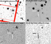 |
Fig. 1. Top left: Pan-STARRS reference i-band image of the host of SN 2018bsz (the red pixels are bad pixels or chip gaps). Top right: ATLAS target image from 2018 May 23. Bottom left: ATLAS difference image obtained on 2018 April 11, showing a clear detection of SN 2018bsz. Bottom right: ATLAS difference image obtained on 2018 March 30 showing the 4-sigma detection. |
The explosion date is then estimated as the mid-point between the epoch of last non detection and that of discovery, with the error being half the difference in time between the points. We therefore adopt an estimated explosion epoch for SN 2018bsz of 2018 March 25, MJD = 58202.5±5. It is important to note that we cannot rule out a significantly earlier epoch with SN 2018bsz evolving at magnitudes below our photometric limits. This would require a steeper initial rise before the “long duration plateau” (the latter is characterised in Sect. 4). However, the value of the true explosion date and the nature of any prior unseen light-curve evolution does not strongly affect our main results and conclusions.
Initial spectral classifications were made on 2018 May 20 (Hiramatsu et al. 2018; Clark et al. 2018) by both the Las Cumbres Global Supernova Project, and ePESSTO3, the extended Public ESO Spectroscopic Survey for Transient Objects (Smartt et al. 2015). Both reports concluded SN 2018bsz was a young SN II due to a strong P-Cygni spectral line profile at a wavelength consistent with Hα (see spectra in Fig. 2). At the redshift of the host galaxy (0.0267), this made SN 2018bsz a bright SN II. However, further inspection of the spectral features cast doubt on this initial classification.
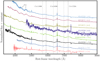 |
Fig. 2. Optical wavelength spectral sequence of SN 2018bsz: from nine days before to seven days after maximum light (MJD = 58267.5 in r). Dotted vertical black lines indicate the rest wavelength of three C II lines, while the dashed vertical grey lines indicate the same C II lines at a velocity of –11 000 km s−1. Two additional lines are clearly observed between 4000 and 5000 Å that are most likely associated with O II. Narrow emission is visible due to an underlying host H II region (see e.g. Hα, Hβ) and is not associated with the transient itself. Additional line identifications are presented in Fig. 5. Spectra have been corrected for line of sight extinction, both in our own Milky Way and from within the host galaxy of SN 2018bsz. We do not plot two spectra obtained with SPRAT at +3 days and with FLOYDS at +3 days, due to their low S/N (but their details are listed in Table A.1 and the spectra will be released). The X-Shooter spectra have been binned to 6 Å in wavelength. |
A clear bump is visible to the red of Hα, that is not generally observed in SNe II. Hβ is usually stronger in absorption than Hα in early-time SN II spectra (see e.g. Gutiérrez et al. 2017), however there is no evidence for this line in any of the spectra of SN 2018bsz (see Fig. 2). (In SLSNe-II Hα is also always accompanied by strong Hβ: Miller et al. 2009; Gezari et al. 2009; Terreran et al. 2017; Inserra et al. 2018a.) There are a number of spectral lines observed between 4000 and 5000 Å that are hard to interpret within a SN II classification. Comparing the classification spectrum to SLSN spectral models of Dessart (in preparation, see Sect. 5), suggested that the strong P-Cygni feature at around 6500 Å could be C II λ6580, with additional C II features also identified. The Supernova Identification (SNID, Blondin & Tonry 2007) software package was used and good matches were found between SN 2018bsz (using the earliest spectrum; nine days before maximum) and several SLSNe, including PTF12dam at 15 days before maximum and PTF09atu at 20 days before maximum. In addition, SN 2018bsz continued to rise to an absolute magnitude of –20.5 mag (in B, after correction for Milky-Way and host-galaxy extinction, see Sect. 3.2). This brightness falls at the low end of the distribution of SLSN-I luminosities (De Cia et al. 2018; Inserra et al. 2018a) but is still much brighter than canonical SNe Ic (and core-collapse events in general; Richardson et al. 2014). These properties led to a reclassification of SN 2018bsz to a SLSN-I (Anderson et al. 2018).
3. Spectral properties of SN 2018bsz
3.1. Spectral observations
In Fig. 2 we present the optical-wavelength spectral sequence of SN 2018bsz. Details of this sequence are listed in Table A.1. These data were obtained and reduced through standard procedures. FLOYDS spectra from the Las Cumbres Observatory (Brown et al. 2013) Global Supernova Project were reduced as in Valenti et al. (2014), while EFOSC2 (Buzzoni et al. 1984, mounted on the NTT) spectra were reduced using a custom built pipeline for the PESSTO project (Smartt et al. 2015). Spectra obtained by the Spectrograph for the Rapid Acquisition of Transients (SPRAT; Piascik et al. 2014) on the Liverpool Telescope (Steele et al. 2004) were reduced using the standard SPRAT pipeline. IMACS (mounted on the Magellan telescope) was used in its short camera configuration (f/2) with a 0.9″ slit and the 300 l mm−1 blue grism. Reductions were achieved using standard IRAF 4 routines. Near-UV, optical and near-IR spectroscopic observations carried out with X-Shooter (Vernet et al. 2011, on the VLT) were obtained in a single 900 s exposure, using 1.0 × 11″, 0.9 × 11″, and 0.9 × 11″ slits for the UVB, VIS, and NIR arms respectively. The spectra were reduced as outlined in Selsing et al. (2018), including: recalibrating the wavelength solution, correcting for slit losses, and correcting for telluric absorption.
Near-IR wavelength spectra were obtained at three epochs and are presented in Fig. 3 (see Table A.1 for details). The FLAMINGOS-2 (Eikenberry et al. 2008, on the Gemini telescope) spectrum was taken in longslit mode with the JH grism and filter in place, with a slit width of 0.72″, yielding a wavelength range of 1.0–1.8 μm and R ~1000. The data were obtained at the parallactic angle with a standard ABBA pattern for sky subtraction. The total exposure time was 12 × 120 s. The data were reduced in a standard way using the FLAMINGOS-2 PyRAF package provided by the Gemini observatory. Telluric corrections and flux calibration were determined with an A0V star observed adjacent in time to the SN 2018bsz data, using the telluric correction methodology of Vacca et al. (2003). The FIRE (mounted on the Magellan telescope) spectrum was taken with the high throughput long slit mode with 0.6″ slit width. A total of 4 sets of ABBA were obtained, with per frame exposure time of 126.8 s, making a total on-target exposure time of 2028.8 s. The A0V star, HD 148733, was used as the telluric and flux standard, and standard reduction routines were followed. All spectral observations will be made public via WISeREP (Yaron & Gal-Yam 2012)5
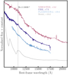 |
Fig. 3. Near-IR spectral sequence of SN 2018bsz. We also plot the model of Dessart (in preparation) that is discussed in Sect. 5. The rest wavelength of He I λ 10830 is indicated. |
3.2. Spectral-line identification, time evolution, and comparison to other SLSNe
A number of strong features are observed in the optical spectra. Specifically, we identify C II lines at wavelengths of ~5890 Å, ~6580 Å and ~7234 Å. These C II lines show consistent blue-shifted absorption troughs at around 11 000 km s−1 (Fig. 2) in the spectra obtained around a week before maximum light (alternatively, around 55 days post explosion), which are typical of SLSNe-I near to peak (Gal-Yam 2018). Such strong carbon lines have been predicted by spectral models (Dessart et al. 2012; Mazzali et al. 2016), but have rarely been detected at such strength (but see Nicholl et al. 2016, for identification of C II in SN 2015bn, together with Yan et al. 2017 where a number of C II lines are detected and characterised in Gaia16apd).
SLSN-I spectra are usually characterised as having relatively strong spectral features between 3500 and 5000 Å associated with O II and formed by many tens of overlapping lines (see modelling of Mazzali et al. 2016 for lists of line identifications). The characteristic “w-shape” produced by these O II lines is seen in the early-time spectra of SN 2018bsz, however the whole feature appears shifted to redder wavelengths than usual (Fig. 4, although they do nicely align with PTF10aagc as will be discussed below). The features usually associated with O II are formed by many tens of overlapping lines. The absorption minima are formed at wavelengths where these multiple O II lines are blue shifted to, with peaks seen at spaces where O II contributions are not present (Gal-Yam 2018). Figure 4 clearly shows that the wavelengths of the peaks in these regions for SN 2018bsz (dashed vertical grey lines) align with the wavelengths of troughs (absorption) for the two well-observed nearby SLSNe-I: Gaia16apd and SN 2017egm.
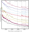 |
Fig. 4. Spectral comparison between SN 2018bsz at –9 day (from maximum light) and SLSNe of the best SNID matches together with three well observed, nearby literature events, and a well-observed fast-evolving SLSN-I. The rest wavelength of the three most prominent C II lines are shown by dotted black lines, while the peaks and troughs of the w-shaped O II feature for SN 2018bsz are indicated by dashed and dotted grey lines respectively. The latter enables a direct comparison to the peaks and troughs found in other SLSNe-I. References: PTF12dam (Quimby et al. 2018); PTF10aagc (Quimby et al. 2018); SN 2009jh (Quimby et al. 2018), these first three are smoothed spectra; SSS120810 (full name SSS120810-231802-560926, Nicholl et al. 2014), Gaia16apd (Kangas et al. 2017); SN 2015bn (Nicholl et al. 2016); SN 2017egm (Bose et al. 2018); LSQ14mo (Chen et al. 2017a). |
The reasons for these clear offsets are not obvious. Assuming the first absorption trough in SN 2018bsz and Gaia16apd as one moves blue ward of Hβ is produced by the same feature, then comparing the wavelength of these absorption troughs one obtains a velocity difference of more than 10 000 km s−1, which is too large to be explained through ejectavelocity differences. It is possible that a change in the morphology of the spectrum in this wavelength region (between SNe) may be produced through differences in ejecta density profiles. In addition, differences could be caused by overlapping lines such as Fe III. Finally, identifying these features as the same O II lines in different SLSNe-I may be in error. We leave a more indepth study of this latter possibility for future work.
The near-IR spectra (Fig. 3) are almost completely featureless. In Fig. 3 we indicate the rest wavelength of He I λ 10830, and there is a small feature in the observed spectra slightly to the red that can most easily be seen in the FLAMINGOS-2 spectrum. We do not claim a clear detection of any line here (whether it be He I λ 10830 or something else), but we do note that He I λ 10830 is relatively strong in the spectral model (displayed in Fig. 3 and discussed in more detail below), possibly supporting the line detection and identification. Spectral-line detections at such wavelengths in SLSNe-I have previously been claimed for SN 2012il by Inserra et al. (2013) and in SN 2015bn by Nicholl et al. (2016). However, similarly to SN 2018bsz, an identification with He I λ 10830 is still not clear.
In Fig. 5 we plot three of the highest S/N optical-wavelength spectra that we have obtained of SN 2018bsz that also cover the full range of epochs at which SN 2018bsz has been observed. The three clearly detected C II lines discussed above (λ 5890, λ6580 and λ7234) do not appear to change visually in shape or strength over the 16 day time range. Measuring line velocities from the minimum flux of absorption (by fitting a Gaussian to the line using IRAF), we find that on average absorption velocities go down by 3000 km s−1 from eight days before to three days after maximum light, to around 8000 km s−1. There is little evolution between four and seven days post maximum.
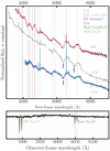 |
Fig. 5. Top: SN 2018bsz optical-wavelength spectra obtained at eight days prior to maximum light, three days after maximum light, and one week post maximum. The positions of host H II region emission lines (not associated with the SN) are indicated as dashed blue vertical lines, while narrow absorption from Milky-Way Na I D absorption is shown as a dashed yellow line (and a zoom also showing such absorption within the host is presented in the bottom panel). C II line rest wavelengths are indicated by grey vertical lines, while the position of both the peaks and the troughs of the O II features is shown in red. We also identify relatively narrow emission features in the absorption troughs of C II, that we label as “High Velocity, HV” features. Narrow calcium H + K absorption from within the host galaxy is also observed. Bottom: a zoom of the spectral region between 5800 Å and 6150 Å as seen in the X-shooter spectrum (three days post maximum). The latter shows the clear detection of sodium absorption within the host galaxy of SN 2018bsz, together with the strong MW sodium absorption. |
Defining the wavelength of minimum absorption is complicated by the presence of small, narrow emission features directly within the absorption trough of C II λ6580 and possibly C II λ7234, as indicated by the dark blue lines in Fig. 5. These features are most prominent in the X-shooter (+3 days) and IMACS (+7 days) spectra, but can also be identified in the EFOSC2 spectrum eight days before maximum. Analysing this feature in the X-shooter spectrum (that of the highest spectral resolution), we measure a FWHM of the emission of 2300 km s−1, and the peak of the emission falls at a rest wavelength of 6400 Å. We tentatively identify these as High-Velocity (HV) features of C II being formed in a detached shell of material at almost 9000 km s−1 (as compared to the bulk ejecta velocities of around 8000 km s−1 at these epochs).
In the bottom panel of Fig. 5 we present the X-shooter spectrum in the wavelength range 5800–6510 Å in order to show the wavelength region of absorption from the sodium doublet (Na I D). Absorption is clearly observed at both rest-frame wavelength of the doublet (λλ 5896,5890) and at the redshift of SN 2018bsz (the absorption is also clearly seen in the IMACS spectrum). Measuring the equivalent widths of each line, for the Milky-Way absorption we estimate a total Na I D EW of 0.91 Å. Using this value, together with the relation from Poznanski et al. (2012) we obtain a E(B − V) = 0.164 mag that is somewhat lower but still consistent with the value quoted above taken from Schlafly & Finkbeiner (2011; given the dispersion on the Poznanski et al. 2012 relation together with our measurement errors). The detection of Na I D absorption within the host of SN 2018bsz is the first time (to our knowledge) such absorption has been identified in spectra of SLSNe-I. Host galaxy extinction is usually assumed to be negligible in SLSN hosts (Leloudas et al. 2015; Nicholl et al. 2015a; De Cia et al. 2018). At the redshift of the host galaxy we measure a total EW (summing the two lines) of 0.40 Å. This translates to a E(B − V) = 0.041 mag along the line of sight to SN 2018bsz within the host galaxy. We use this value to further correct spectra and photometry for host galaxy line-of-sight extinction. In addition to Na I D absorption, we also observe Ca II H and K absorption (at 3966, 3934 Å) at the redshift of the host. A deeper analysis of these narrow interstellar (or circumstellar) lines and a search for possible time variability, will be the focus of future work.
As outlined above, our reclassification of SN 2018bsz was aided by comparison to spectral templates using SNID (Blondin & Tonry 2007), together with the comparison to spectral models (Dessart, in prep.). In order to find similar events we searched the Open Supernova Catalog (Guillochon et al. 2017) for all SLSN-I with more than three spectra of reasonable S/N (in order to have various phases of the template SNe covered). These spectra were then converted into templates for SNID, and a comparison was made between SN 2018bsz and other SLSN spectra (together with the full range of other SN spectral templates: those originally available in SNID plus those from Liu et al. 2016, 2017 and Gutiérrez et al. 2017). The best matches (according to SNID but then confirmed visually6) are compared to SN 2018bsz in Fig. 4, together with those from an additional three well-observed nearby SLSNe-I. Reasonable matches were found to: SN 2009jh; PTF12dam; and SSS120810 (references for these SNe are listed in the figure caption). The best match was found with PTF10aagc. PTF10aagc clearly shows spectral features at similar wavelengths to SN 2018bsz, specifically C II λ5890 λ6580 and λ7234, however the emission peaks appear to be consistently blue shifted. PTF10aagc also shows similarities to SN 2018bsz in the wavelength position of the features at around 4500 Å. Similarly to SN 2018bsz (see below), PTF10aagc was relatively low-luminosity for a SLSN, with a peak rest-frame g-band brightness of –20.1 mag (De Cia et al. 2018). While PTF10aagc lacks pre-maximum data, its post-peak observations showed two interesting properties. First, PTF10aggc evolved extremely rapidly, being one of the fastest events in the sample of De Cia et al. (2018). Here we do not discuss in any detail the evolution of SN 2018bsz after maximum light, however there are already some indications that it will fall into the “fast” evolving group of SLSNe-I. Second, in spectra obtained several months after maximum PTF10aagc developed clear hydrogen features, with convincing detections of both Hα and Hβ (Yan et al. 2015; Quimby et al. 2018). We await the post-peak spectral evolution of SN 2018bsz to see if it reveals similar features.
While a number of SLSNe-I were found to match the early-time spectra of SN 2018bsz, the three nearby events: SN 2015bn (Nicholl et al. 2016), Gaia16apd (Kangas et al. 2017), and SN 2017egm (Bose et al. 2018), which we also compare to in Fig. 4 show similarities but clear differences. Indeed, Gaia16apd can be found to match spectra of SN 2018bsz, but only if redshift is allowed to vary enabling the 4000–5000 Å features to match (SNID gives matches with SN 2018bsz to many SLSNe-I but at significantly different redshifts to its host). This again highlights the issue discussed above: the O II identifications in SN 2018bsz are quite distinct from those in other nearby SLSNe. Gaia16apd was as an intermediate object in terms of its light-curve evolution; in between those of fast and slow evolving SLSNe-I, while being relativity bright at a g-band absolute magnitude of –21.8 mag (Kangas et al. 2017). As shown in Fig. 4, Gaia16apd displayed strong O II features with peaks and troughs at significantly different rest wavelengths to SN 2018bsz. A number of C II features were identified in Gaia16apd by Yan et al. (2017), but weaker than in SN 2018bsz.
SN 2015bn was intrinsically brighter than the general SLSN-I population (at M U of around –23.1 mag), faded slowly, and displayed significant variability in its decline post-peak (Nicholl et al. 2016). C II λ7234 was identified (Nicholl et al. 2016) and a hump can clearly be seen in Fig. 4 at these wavelengths. However, no significant C II λ6580 was observed. SN 2015bn showed relatively strong O I λ7774 absorption that is not seen in SN 2018bsz.
Similar to SN 2018bsz, SN 2017egm was relatively faint for a SLSN-I (Bose et al. 2018). C II was tentatively identified by Bose et al. (2018) in the earliest spectrum of SN 2017egm, and clear absorption related to C II λ6580 developed around maximum light, however none of the C II features were as strong as seen in SN 2018bsz. LSQ14mo is also displayed in Fig. 4 as an example of a well-observed fast-evolving SLSN-I (Chen et al. 2017a). LSQ14mo does not show any signs of strong C II. However, perhaps interestingly LSQ14mo displays O II-line morphology similar to SN 2018bsz. A full analysis of how SN 2018bsz fits into the overall picture of SLSNe-I will be possible when the full post-peak evolution has been observed.
4. SN 2018bsz photometric properties
4.1. Photometric data
UV, optical and near-IR photometry of SN 2018bsz were obtained from a range of different telescopes and instruments. Photometry for each instrument is listed in the tables in the appendix. ATLAS photometry is measured from point-spread-function fitting through tphot (Merlin et al. 2015) applied to the difference images. The orange and cyan filters and the photometric calibration are described in Tonry et al. (2018), and the magnitudes are on the AB system. ATLAS typically observes each region of sky 4 times per night in 30 s exposures over a ~1 h period and we report the nightly mean magnitude here (Table B.1).
Near UV photometry was obtained using the Neil Gehrels Swift Observatory on 2018 May 31, and 2018 June 3. The transient was bright in all near-UV (NUV) and optical filters of the Swift/UVOT telescope. The UVOT data were reduced using the standard pipeline available in the HEAsoft software package7. The observation on May 31 was conducted during 3 orbits while the observation on June 3 was conducted during 2 orbits. To improve the S/N ratio of the observation in a given band in a particular epoch we co-added all orbit-data for that corresponding epoch using the HEAsoft routine uvotimsum. We used the routine uvotdetect to determine the correct position8 of the transient and used the routine uvotsource to measure the apparent magnitude of the transient by performing aperture photometry. For source extraction we used an aperture with a radius 4.7 arcsec while to determine the background an aperture of radius 127.8 arcsec was used. Magnitudes listed in Table B.4 are on the AB system. We note that the UVOT photometry is not host subtracted.
We monitored the JHK light curve evolution of SN 2018bsz using the Gamma-Ray Burst Optical/Near-Infrared Detector (GROND; Greiner et al. 2008), mounted at the 2.2 m MPG telescope at the ESO La Silla Observatory in Chile. The images were reduced using the GROND pipeline (Krühler et al. 2008), which applies de-bias and flat-field corrections, stacks images and provides astrometry calibration. The SN magnitudes are calibrated against 2MASS field stars and are listed in Table B.5 in the AB system.
Las Cumbres Observatory UBVgri-band data were obtained with Sinistro cameras on the 1 m telescopes, through the Global Supernova Project. Using lcogtsnpipe (Valenti et al. 2016), a PyRAF-based photometric reduction pipeline, PSF fitting was performed. UBV-band data were calibrated to Vega magnitudes (Stetson 2000) using standard fields observed on the same night by the same telescope. gri-band data were calibrated to AB magnitudes using the AAVSO Photometric All-Sky Survey (APASS, Henden et al. 2009). Sinistro photometry is listed in Table B.3. It is important to note that the Sinistro photometry is not hostgalaxy subtracted due to a lack of host templates.
SkyMapper photometry was extracted from images from the Transient Survey (Scalzo et al. 2017) and the Southern Survey (Wolf et al. 2018) taken using the set of uvgriz filters available at the telescope. Images were reduced using the pipeline described in Wolf et al. (2018), where the photometric extraction and calibration methodology is also outlined. Magnitudes are obtained in the AB system, where zeropoint calibration is anchored to APASS DR9 and 2MASS. We note that the SkyMapper photometry is not host subtracted.
4.2. The SN 2018bsz light curve, colours, and temperatures
The NUV, optical and near-IR light curves of SN 2018bsz are displayed in Fig. 6. To produce the absolute-magnitude light curves the data were corrected for a host galaxy distance modulus of 35.23, a Milky-Way reddening of E(B − V) = 0.214 mag (Schlafly & Finkbeiner 2011), and an E(B − V) = 0.041 mag internal to the host (a bolometric light curve is presented in Section 5). The first detection gives an initial rise of 1.5 mag in five days (assuming an explosion epoch of 2018 March 25). The light curve then flattens, and a clear slowly rising “plateau” is observed from five to 33 days post explosion, equating to a duration of 26 days, that could easily be extended to around 40 days depending on which photometric data one includes in the assessment. During this plateau SN 2018bsz displays a relatively slow rise of 0.89 o-band magnitudes in 26 days (at a rate of 0.034 mag d−1), with an absolute magnitude of around –18 at around 25 days post explosion (40 days pre-maximum). A significant change in the lightcurve shape is observed at just after 40 days, with the rise significantly steepening. The light curve increases in brightness by an additional two magnitudes in 18 days (at a rate of 0.12 mag d−1). At peak (MJD = 58267.5, estimated from fitting a low-order polynomial to the r-band photometry) SN 2018bsz is –20.3 mag in the ATLAS o band. SN 2018bsz has an absolute peak magnitude of –20.5 in the B band and –20.3 in the r band.
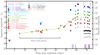 |
Fig. 6. UV, optical and near-IR light curves of SN 2018bsz. All photometry is corrected for both Milky Way and host galaxy line of sight extinction. Epochs of optical spectroscopy are shown as blue lines on the x-axis, while epochs of near-IR spectroscopy are indicated by red lines. The upper limit of the most recent non-detection prior to discovery is shown as a maroon upside-down triangle. |
SN 2018bsz thus has a relatively low absolute magnitude. Formally, this is significantly lower than the initial operational limit of –21 mag (at optical wavelengths) used to include SNe in the super-luminous category (Quimby et al. 2011; Gal-Yam 2012). However, as outlined in the introduction, SLSNe are now more generally defined by spectroscopic properties, and while SN 2018bsz is somewhat spectroscopically abnormal compared to the general SLSN-I population (Sect. 3.2), it clearly shows similarities to SLSNe-I, as suggested by the SNID matches. The sample analyses of Inserra et al. (2018a), Lunnan et al. (2018), and De Cia et al. (2018) include a number of events dimmer than –21 mag, and SN 2018bsz falls within the published distributions while being a relatively low-luminosity SLSN-I. We also note that there exists a number of very bright SNe Ic that are generally not considered SLSNe. Two examples are SN 2012aa (Roy et al. 2016) and SN 2011kl (Greiner et al. 2015) that both peaked at around –20 mag. Understanding the link between luminous SNe Ic and under-luminous SLSNe-I may give important clues to the physics of these different classes of explosions. Swift photometry three days post maximum gives an absolute uvw1 (central wavelength of 2600 Å) magnitude of –20.4. Comparison to figure 6 of Smith et al. (2018) suggests that SN 2018bsz is offset to lower luminosity than the rest of the sample, by almost one magnitude. The post-maximum near-IR light curve is relatively flat with little change in brightness over the ~1-week duration of the observations.
Using the estimated epoch of maximum brightness in the r-band gives a rise time of 63 rest-frame days. This is quite typical for SLSNe-I as shown in Fig. 7 and is close to the representative value used in De Cia et al. (2018). However, a number of SLSNe-I with both significantly longer and shorter rise times have been observed. The latest photometry displayed in Fig. 6 indicates that SN 2018bsz is now clearly past maximum light and has started to decline. A characterisation of the post-maximum light curve awaits further data.
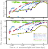 |
Fig. 7. Comparison of the pre-maximum light curve of SN 2018bsz to those of SLSNe-I from the literature showing clear bumps before the main rise to maximum (iPTF13dcc is shown in open circles as its form is clearly distinct from the events). Next to each SLSN name in parenthesis we give the object redshift (in the bottom panel). Non-detection upper limits are indicated by upside down triangles. Top: light-curves normalised to maximum-light magnitude. Bottom: absolute magnitude light curves with respect to maximum light. SN 2018bsz is in the ATLAS o band, while all other comparison SNe are in observed R or r band. Given the range of redshifts of the SLSN comparison sample, these observed bands equate to different rest frame wavelengths. However, given the lack of a) multi-band photometry (to enable rest-frame band comparison) and b) spectra of SLSNe-I during these epochs (to allow for valid K-corrections) we prefer to plot the data in its “raw” form. Colour effects may complicate the direct comparison of these light curves. |
We estimate the observed colours (corrected for Milky Way and host galaxy extinction) of SN 2018bsz at four epochs: during the plateau; at the start of the second steeper rise; at maximum light (in the r band); and from our last photometric data obtained at eight days post maximum. At around 25 days post explosion/40 days before maximum SkyMapper multi-band photometry is available. This gives a u − g colour of 0.58 mag at the mid-point of the initial slower rise/plateau (see Fig. 6). At around 55 days post explosion or ten days before maximum (when the light curve has clearly started to steepen its rise), the u − g colour becomes much bluer, at –0.16 mag. SN 2018bsz continues to get bluer with a U − g colour (note here we are using Las Cumbres Observatory photometry and no longer SkyMapper) at maximum light of –0.54. The last epoch of photometry included in this paper, at eight days post maximum, shows that the SN has started to get redder again with a U − g colour of –0.44 mag.
To estimate black-body temperatures we extract spectral energy distributions (SEDs) from the NUV and optical photometry of SN 2018bsz at the same epochs for which we cite colours in the previous paragraph. Temperature errors are estimated through combining those obtained through Monte Carlo simulations sampling values from the photometry and their errors together with those obtained by removing the bluest and reddest photometric bands and reestimating temperatures. At the earliest epoch where we have more than two photometric points – at around 25 days post explosion or 40 days before maximum – using SkyMapper uvgr photometry we estimate relatively cool black-body temperature of 6700±1000 K. This rises to 13 300±940 K after the light curve has started the main rise to maximum (at around 50 days post explosion or 10 days before maximum, again estimated using SkyMapper photometry but now uvgriz). At around maximum light a temperature of 9500 ± 180 K is obtained (now using Las Cumbres photometry; UBVgri), while at eight days post maximum the temperature cools to 8800 ± 200 K (again using Las Cumbres UBVgri photometry).
The estimated temperature changes are consistent with the colour changes outlined above. Black-body fitting to spectra produces similar results. Overall, we observe that SN 2018bsz was quite red and cool during it’s long-duration plateau, but quickly became blue and hot as the rise steepened to maximum light. However, we note that the SkyMapper and Las Cumbres photometry have not been subtracted of the underlying host emission, and this is probably affecting the estimated colours. Indeed, ATLAS photometry – that is host-galaxy subtracted – gives c − o ≈ 0 at almost the same plateau epoch of 25 days post explosion. This is bluer than the colour from SkyMapper, and implies a temperature in excess of 9000 K. In addition, the ATLAS colour does not change significantly from the plateau to the start of the rise to peak, in contrast to the SkyMapper and Las Cumbres colours. Therefore the above colours, blackbody temperatures and their time evolution should be evaluated with some caution and a full discussion of these parameters for SN 2018bsz will only be possible when all presented SN photometry is host-galaxy subtracted in the future. At the same time, it seems unlikely that the temperature during the plateau is much higher than 10 000 K, and this suggests that overall SN 2018bsz is relatively red at these epochs, while during the main rise it also appear to be likely that SN 2018bsz does not reach the high temperatures of 15–20 000 K reached by other SLSNe-I (Howell 2017; Bose et al. 2018).
4.3. The pre-maximum light curve of SN 2018bsz compared to other SLSNe-I
As discussed above, SN 2018bsz shows a clear, long-duration rising plateau before the second steeper rise to maximum light. Pre-rise “bumps” or “excess emission” have previously been observed in a number of SLSNe-I (Leloudas et al. 2012; Nicholl et al. 2015b; Nicholl & Smartt 2016; Smith et al. 2016; Vreeswijk et al. 2017; Lunnan et al. 2018). However, the feature observed in SN 2018bsz is not well described by the term bump as it has a linear form (in magnitudes) for at least 26 days (and up to 40 days) before the steeper rise to maximum starts. As shown in the previous section, the colour of SN 2018bsz during this initial epoch is relatively red implying a relatively low black-body temperature.
Figure 7 compares ATLAS photometry of SN 2018bsz to that of five other SLSNe from the literature that showed clear signs of an early-time bump before the main rise to maximum light. (We note, the photometry from this comparison sample are not K-corrected, leading to a strong caveat to some of the subsequent discussion: all comparison SNe are shown in observed-frame r or R band.) There are two properties that mark SN 2018bsz as being different from these previously discussed bumps. First, the feature in SN 2018bsz appears to be of significantly longer duration. Taking the minimum length of the observed plateau of SN 2018bsz to be 26 days, this is then around ten days longer than any of the comparison sample. Secondly, the absolute magnitude at the mid-point of this plateau is around –18 mag (in ATLAS o band).
Most other events are significantly brighter than SN 2018bsz (both at this epoch but also at maximum; see also events in Lunnan et al. 2018), with only PTF12dam (Vreeswijk et al. 2017) displaying similar luminosity pre-rise emission. However, in the case of PTF12dam, the strong constraint on the explosion epoch suggests that this bump was only of around 10 days in duration (while the upper limit plotted in Fig. 7 is only 0.5 mag fainter than the first detection, a non-detection three days before has an upper limit 1.8 mag fainter, hence ruling out an unobserved longer-duration plateau).
SN 2006oz (Leloudas et al. 2012) shows a light-curve morphology somewhat similar to SN 2018bsz (see top panel of Fig. 7), but brighter by around a magnitude both at maximum and during the plateau (bottom panel of Fig. 7). The upper-limit on the non detection of SN 2006oz prior to discovery is only 0.6 mag lower than the first detection. This suggests the possibility that the bump in SN 2006oz could have extended further back in time but was below our detection limits. However, Leloudas et al. (2012) constrained the temperature to be around 15 000 K during these early epochs; higher than that of SN 2018bsz.
The case of LSQ14dbq (Nicholl et al. 2015b) is clearly distinct, as this SN displayed a very pronounced first peak of around 10 days duration before declining then rising again to the second brighter maximum. Finally, DES14X3taz (Smith et al. 2016) displays a somewhat similar light-curve morphology to SN 2018bsz, while being more than a magnitude brighter. However, in this case the upper limit prior to the start of this bump rules out a more extended plateau as observed in SN 2018bsz. In addition, similarly to the case of SN 2006oz: DES14X3taz was constrained to have a significantly higher temperature during this bump.
While we plot iPTF13dcc (Vreeswijk et al. 2017) in Fig. 7 (given that it is often discussed within this context in the literature), we do not discuss it any further here, given that the lightcurve morphology is quite distinct from the other events shown. Overall, we conclude that the relatively red, long-duration slow rise (plateau) seen in SN 2018bsz is unprecedented in SLSNe-I observed to date.
Aware of the clear uniqueness of the early-time light curve of SN 2018bsz, we now briefly discuss previous models suggested to explain bumps in the early-time light curves of other SLSNe (a full exploration of possible models to explain the peculiar properties of SN 2018bsz is beyond the scope of this initial discovery paper). One option is that the initial plateau is simply the initial “normal” core-collapse SN of for example type Ic (to match the later carbon-dominated spectra). In the cases of LSQ14bdq and DES14X3taz this possibility was ruled out due to the high luminosity and very large 56Ni mass required (Nicholl et al. 2015b; Smith et al. 2016). SN 2018bsz is significantly dimmer during the early-time light curve, at a luminosity similar to some SNe Ibc (Richardson et al. 2014).
In Fig. 8 we plot three example SNe Ic. SN 1998bw was a broad-line SN Ic associated with a Gamma-Ray Burst (data obtained from Patat et al. 2001), SN 2007gr was a normal SN Ic (Valenti et al. 2008), and SN 2011bm was a slowly evolving SN Ic (Valenti et al. 2012). We plot these SNe Ic both with respect to epoch of maximum (as done for all SLSNe-I in the figure) and with respect to explosion epoch. The latter is done to specifically see how well a SN Ic light curve may be able to explain the early-time pre-maximum light curve of SN 2018bsz. SN 1998bw is significantly brighter than SN 2018bsz at 10–20 days after explosion, and the morphology of the light curves are also distinct. SN 2007gr has a similar luminosity 10–15 days after explosion, but quickly declines while SN 2018bsz continues to rise. Meanwhile, SN 2011bm matches the pre-maximum light curve of SN 2018bsz reasonably well. The latter is somewhat flatter and shows no clear peak before the rise steepens to maximum, however the differences between SN 2018bsz and SN 2011bm are not so big.
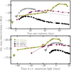 |
Fig. 8. Comparison of light curve of SN 2018bsz to SNe Ic: SN 1998bw, a broad-line event associated with a long-duration Gamma-Ray Burst; SN 2007gr, a typical SN Ic; and SN 2011bm, a slowly evolving SN Ic. Top: light curves with respect to estimated explosion epoch. Bottom: light curves with respect to epoch of maximum light |
We estimate the black-body temperature of SN 2011bm from the available multi-band photometry as achieved for SN 2018bsz above at a similar epoch (post explosion) to the plateau temperature of SN 2018bsz. In the case of SN 2011bm we obtain a temperature of 7200 ± 650 K that is consistent with that of SN 2018bsz at a similar epoch (6700±1000 K, although note the above caveats). Hence, we suggest the possibility that the plateau in SN 2018bsz could have been produced by a SN Ic-like explosion, where the following steeper brightening is due to a secondary (possibly central) power source that starts to dominate at later times. In the case of SN 2011bm, Valenti et al. (2012) estimated a massive ejecta and therefore a very large initial progenitor mass from the broad light curve. As an additional note of interest Fig. 8 (bottom panel) shows that with respect to maximum light epoch the light curve of SN 1998bw has a very similar morphology to that of SN 2018bsz only at lower luminosity.
Previously, a more favoured model for other SLSNe-I showing signs of excess emission pre-maximum has been that of shock cooling of extended material around the progenitor (see Leloudas et al. 2012; Nicholl et al. 2015b; Smith et al. 2016 and the analytic model of Piro 2015). In the case of SN 2018bsz, shock-cooling has to be extended to much longer durations and produce a slowly rising light curve. It is not clear that shock cooling can produce such a light curve. Kasen et al. (2016) suggested that a magnetar-driven shock breakout could produce doublepeaked light curves such as that observed in LSQ14dbq. However, these models predict temperatures of around 20 000 K during the first peak; much higher than the colour/temperature observed in SN 2018bsz making the Kasen et al. (2016) scenario unlikely.
5. Comparison to synthetic spectra
The reclassification of SN 2018bsz to a SLSN-I was partially driven by comparison to model spectra, specifically the identification of strong C II lines as outlined above. In Fig. 9 we show a comparison between the observed spectrum obtained eight days before maximum light and a model spectrum that qualitatively shows similar line features. (The model spectrum is taken at 43 days post explosion, which corresponds to more than a week post maximum: later we discuss the clear differences between the model and SN 2018bsz after discussing the similarities in the spectra.) This spectrum was taken from radiative transfer simulations from a theoretical study on magnetar powered SNe of Type Ic (Dessart, in preparation).
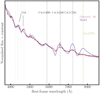 |
Fig. 9. Comparison of an optical-wavelength spectrum of SN 2018bsz with a model spectrum from Dessart (in preparation). C II line rest-frame wavelengths are indicated by black dotted vertical lines. In the case of the O II lines we draw vertical grey dashed lines that align with the peaks in the spectra and vertical grey dotted lines for the troughs (absorption). O I λ7774 is clearly observed in the model, but not in the observations, and is indicated by the vertical yellow dashed line. (The model spectrum is at around 40 days post explosion and around 10 days post maximum and therefore does not correspond to the same exact epoch of the observed spectrum of SN 2018bsz.) |
The numerical approach for these simulations is similar to that outlined in Dessart (2018). Here, the progenitor we use is hydrogen-deficient. It corresponds to a carbon-rich Wolf-Rayet (WR) star with a final mass of 11.4 M ⊙ at core collapse (model r0 of Dessart et al. 2017, which had a progenitor of solar metallicity). This progenitor star is exploded, with V1D (Livne 1993; Dessart et al. 2010a,b) by means of a piston, producing a kinetic energy of 1.23 × 1052 erg. The kinetic energy is large relative to neutrino-powered SNe but is in line with what magnetorotational explosions may produce (before forming a magnetar; Burrows et al. 2007; Dessart et al. 2008). It contains (in part) the additional kinetic energy – needed to match SLSN ejecta velocities – induced by the magnetar (see below), and ignored by CMFGEN (Hillier & Dessart 2012) (this kinetic energy also matches those used in the spectral modelling of Mazzali et al. 2016). The ejecta composition is dominated by oxygen, with a total oxygen mass of 5.59 M ⊙, and only 0.2 M ⊙ of residual He in the outer ejecta – the He surface mass fraction is 0.19.
At one day after explosion, we remap this ejecta into CMF-GEN and proceed as for the GRB/SN models of Dessart et al. (2017). To make this model deviate drastically from standard SNe Ic, we introduce a magnetar power ė pm. For the magnetar properties, the model is characterised by a magnetic field of 3.5 × 10¹⁴ G and an initial rotation energy of 4.0 × 1050 erg (corresponding to an initial spin period of 7 ms). The spin-down time scale for this model is 19.1 days, the rise time is 25.8 days, and the peak luminosity is 4.86 × 1043 erg s−1. The energy deposition is prescribed rather than solved for Dessart (2018). Depending on the energy deposition profile, the steep light curve rise caused by magnetar power injection can occur within 2–3 days after explosion, or can be delayed by up to 20 days (Dessart, in prep., Fig. 10).
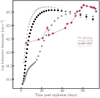 |
Fig. 10. Comparison of model bolometric light curves with that of SN 2018bsz. Model r0e2 is that discussed at length in the text. Model r0e2s is identical but with the magnetar power injected deep within the ejecta with little advection to large velocities, while r0e4 is identical to r0e2 but with higher kinetic energy. There appears to be a jump in the observed light curve at around 25 days post explosion. This is the epoch where multi-band photometry from SkyMapper is available and we see that SN 2018bsz is significantly brighter in r (than other bands). This may be an issue with host galaxy contamination, and we will investigate this further when we are able to perform accurate galaxy-template subtraction when the SN has faded. |
Compared to standard SNe Ic, the influence of the magnetar is to raise the luminosity. Because the initial rotational energy of the magnetar is small compared to the ejecta kinetic energy, the magnetar power changes mostly the internal energy and escaping radiation. The peak luminosity is 10 times greater than in the model without a magnetar. This change is mostly carried by the change in temperature in the spectrum formation region, which also causes a rise in ionisation. The entire SED changes from red (SN Ic) to blue, and the lines we see around maximum are those of O II and C II. For O II, the contributions arise from numerous multiplets around 4000 Å, while the C II lines arise from doublets at 5890 Å, 6580 Å, and triplets at 7235 Å. He I λ5875 contributes negligibly but O I λ7774 is clearly present in the model.
Compared to the observations the model spectrum qualitatively reproduces the main observed features at optical wavelengths (Fig. 9), which we associate with C II and O II. However, we note an offset in wavelength of the peaks of the O II features between the observations and model. As discussed in Sect. 3.2, this inconsistency of the spectral features seen in SN 2018bsz with observations of other SLSNe-I and now spectral models suggests differences in the properties of the line forming regions in SN 2018bsz that should be the focus of future work. O I λ7774 is over predicted by the model. The observed near-IR spectra are almost featureless while the model displays He I λ10830 (that we tentatively identify in observations, Fig. 3) together with a strong feature at around 9000 Å most likely associated with either O I or C III (that is not observed). The strong C II lines observed in SN 2018bsz were also predicted by Dessart et al. (2012), and are usually overestimated relative to observations. Here, it is clear that SN 2018bsz has stronger C II lines than typically seen in SLSNe-I (see Fig. 4). In our models, the strong carbon lines stem from the large carbon mass fraction in the WR progenitor model, either in the present model (computed with MESA; Paxton et al. 2011, 2013, 2015), or the one from Dessart et al. (2012, computed with KEPLER; Woosley et al. 2002) – both are from a 40 M ⊙ star. It will be important for future work to investigate what controls the carbon/oxygen abundance in carbon-rich WR stars and whether this could be used to constrain the evolutionary properties of the progenitor stars.
It is important to note here that the models we use were not tailored to fit SN 2018bsz nor any other particular SN. Firstly, they were produced by exploding progenitors that were the result of standard stellar evolution (in this case using MESA) with the aim of using massive progenitors depleted in both hydrogen and helium (to match spectra of SLSN-I and SNe Ic where the lack of these lines is one of their defining features). Secondly, the exact parameters used to produce models with different properties were chosen to be exploratory; to probe what produces differences in predicted observables. Changes in for example: ejecta mass; magnetar energy deposition; kinetic energy, can significantly change the model results. With these caveats in mind, in Fig. 10 we plot three model bolometric light curves as compared to the observed bolometric light curve of SN 2018bsz (calculated using all available photometry and colours at all epochs, and following the methodology described in Inserra et al. 2018b).
All models have the same composition and are exploded in the same manner as discussed above, however compared to the model above (r0e2) in model r0e2s the magnetar power deposition profile is more confined in velocity space, while model r0e4 is identical to r0e2 but with higher kinetic energy. It is clear that none of the model light curves reproduce that of SN 2018bsz. Most obvious is the long, slow (and bright) rise of SN 2018bsz that is missing in the models, plus the later epoch of maximum light. However, model r0e2s, where the magnetar power is much more confined to the inner ejecta is informative: it shows that a simple change in the way the magnetar energy is deposited can have significant effects on the shape of the light curve. This suggests that fine tuning of the chosen progenitor, explosion and magnetar properties could be able to come closer to the observed properties of SN 2018bsz. One possibility is that this slow rise is indicative of a more massive ejecta with a deeply embedded power source. Of course, there may also be multiple power sources at play producing the observed features of SN 2018bsz.
The model comparison presented in this section shows that the explosion of a carbon-rich WR progenitor can produce spectra qualitatively similar to SN 2018bsz under the correct ionisation conditions. While the timing of these model conditions does not match that SN 2018bsz (in terms of the light-curve evolution), the comparison allows for the identification of strong, persistent C II lines in this nearby SLSN. Understanding what drives the differences between the models and SN 2018bsz can further aid in our understanding of SLSNe.
6. Host galaxy properties
The explosion environments of transients can give clues to their progenitor properties, by constraining their probable ages and metallicities (see Anderson et al. 2015 for a review). Early in the exploration of SLSNe, it was suggested that they prefer dwarf hosts (Neill et al. 2011), and this (together with their intrinsic low rate) is often cited (see e.g. Leloudas et al. 2015) as a reason that they went undetected until around a decade ago, given the previous bias in SN searches to massive, nearby galaxies. Several subsequent studies have analysed samples of SLSNe-I, concluding that their host galaxy properties are biased towards dwarf galaxies of high specific star-formation rate (sSFR) and low, significantly sub-solar metallicity as compared to other SN types and the general galaxy population (Lunnan et al. 2014; Leloudas et al. 2015; Perley et al. 2016; Chen et al. 2017c; Schulze et al. 2018). These studies have suggested that low metallicity may be a prerequisite for the production of SLSN events, perhaps in addition to a young age (Leloudas et al. 2015; Schulze et al. 2018), putting significant constraints on any proposed progenitor model. However, the nearby (the nearest until SN 2018bsz) SLSN-I, SN 2017egm, occurred in a host of relatively high mass and around solar metallicity challenging this picture (Bose et al. 2018; Nicholl et al. 2017; Chen et al. 2017b, although see Izzo et al. 2018). It is in this context that we analyse the host galaxy of SN 2018bsz.
The host galaxy system (2MASX J16093905-3203443) is well-detected and resolved in our supernova follow-up imaging (top panel of Fig. 11). The SN is coincident with what appears to be an isolated spiral dwarf galaxy (17″ or 9 kpc in diameter) with a disturbed morphology, at an offset of 6.8″ from the diffuse nucleus. However, pre-imaging from Pan-STARRS (Fig. 1) makes clear that there is an additional galaxy directly under the SN position concealed by the SN light in the post-explosion imaging (and not distinct in shallow publicly available imaging catalogues, below), suggesting that the system is in fact an ongoing merger of two dwarf galaxies. These properties are reminiscent of many previous SLSN hosts (Lunnan et al. 2014; Perley et al. 2016; Chen et al. 2017a). Detailed characterisation of the host system of SN 2018bsz will be the focus of future work.
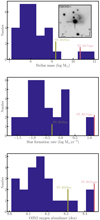 |
Fig. 11. Histograms of the environment and host properties of SN 2018bsz as compared to literature samples and SN 2017egm; the previously lowest-redshift SLSN. Top: integrated host galaxy stellar mass. The inset shows a GROND r-band image of SN 2018bsz (indicated by the two perpendicular black lines) and its host galaxy. Middle: integrated host SFR. Bottom: host environment oxygen abundance on the O3N2 scale (a combination of global galaxy and nearby host H II region measurements). On each plot the value of SN 2018bsz is indicated, together with that of SN 2017egm. |
Additional insight into the nature of the system can be obtained by SED modelling of the multi-wavelength galaxy continuum. The two galaxies are not cleanly separable in preexplosion imaging at most wavelengths, so we model them together as a single system. Data from the UV to the near-IR were obtained from the Galaxy Evolution Explorer (GALEX; Martin et al. 2005), the Two Micron All-Sky Survey (2MASS; Huchra et al. 2012) and the Wide-field Infrared Survey Explorer (WISE; Wright et al. 2010) public databases. Skymapper does not report catalogue photometry for extended objects, so we performed our own photometry on the SkyMapper images using an aperture radius of 29 pixels (14.4″; 7.7 kpc), establishing the photometric calibration by direct comparison to nearby stars in the SkyMapper catalogue (Wolf et al. 2018).
We then fit the broad-band SED of 2MASX J16093905-3203443 using Le Phare (Ilbert et al. 2006) to determine the stellar mass and SFR as in Taggart et al. (in prep.). The results indicate 2MASX J16093905-3203443 is a star-forming, low-mass galaxy with a moderate amount of dust. The galaxy has an absolute r-band magnitude of –19.8 ± 0.24: somewhat brighter than the Large Magellanic Cloud (LMC) but still relatively faint compared to the host population of typical core-collapse supernovae. The stellar mass is  . The SFR is constrained only poorly; we derive
  .
.
We also extract an H II region spectrum from a 2-dimensional SN 2018bsz spectrum in order to derive an environment oxygen abundance. The EFOSC2 spectrum taken at –6 days was used and an emission-line spectrum was extracted from the peak of the galaxy emission (in the 2-dimensional spectrum), at a distance of 3.3 kpc from the SN. Emission-line fluxes were then measured for all H II region lines detected and are listed in Table C.1. Using the O3N2 diagnostic on the Marino et al. (2013) scale we estimate an oxygen abundance of 8.31±0.01 dex (this error is that arising from the measurement error of the line fluxes; the Marino et al. 2013 O3N2 diagnostic gives an additional 0.18 dex systematic error), consistent with around half solar.
In Fig. 11 the environment oxygen abundance, host stellar mass, and host SFR are displayed as compared to samples of SLSNe in the nearby Universe. To create these comparison samples we searched the literature for all SLSNe-I at a redshift lower than 0.3 with published host masses, SFRs and emission line fluxes (with the latter being taken from the exact SN sites if available and global host values if not). Emission-line fluxes were taken from Leloudas et al. (2015), Perley et al. (2016), Chen et al. (2017a), Inserra et al. (2017); and Izzo et al. (2018) and oxygen abundances were calculated on the Marino et al. (2013) O3N2 scale. Host masses and SFRs were estimated using the samples published in Leloudas et al. (2015), Perley et al. (2016), Schulze et al. (2018), however the PTF hosts presented in Perley et al. (2016) were remodelled using Le Phare.Within these distributions we also plot the position of each parameter for SN 2018bsz and SN 2017egm (Taggart et al., in prep.).
As discussed above, SN 2017egm was the previously lowest-redshift SLSN-I and was an outlier in terms of its host galaxy properties, being more massive and more metal rich than the majority of previously observed events. Bose et al. (2018) argued that the absence of similarly low-redshift SLSNe-I in low-metallicity hosts lowered the importance of progenitor metallicity in the production of these events. In contrast, Fig. 11 shows that the host of SN 2018bsz is quite typical of the previously-known SLSN-I host population. While its mass and oxygen abundance are towards the upper end of the distribution from the comparison samples, it is not exceptional. We argue that the small sample of very low-z SLSN-I hosts (two events at z < 0.05) is consistent with our present understanding of the SLSN-I host population based on intermediate-redshift studies.
7. Conclusions
We have presented early-time UV, optical and near-IR data of the lowest-redshift SLSN-I discovered to date, SN 2018bsz. Photometry from the ATLAS survey shows an unprecedented slowly rising (red), long-duration plateau before the main SN peak, with the former being distinct from all other previously analysed bumps in pre-maximum SLSN light curves. The spectra – obtained only after the steeper rise to maximum light had started – display uncharacteristically strong, persistent C II features that are qualitatively similar to those produced by a magnetar-powered explosion of a massive WR progenitor. The host galaxy of SN 2018bsz does not stand out from the general SLSN-I host population, being an intermediate-mass, relatively low metallicity galaxy.
Here, we have analysed and discussed the properties of SN 2018bsz until around a week post maximum light. This nearby SLSN-I will still be visible until mid-October 2018 (before going behind the Sun), and therefore a full multi-wavelength characterisation of the post-peak evolution will be possible. When SN 2018bsz again becomes visible in late January 2019 nebularphase spectroscopy will provide strong constraints on the progenitor star, its explosion, and the power source at the origin of this unique light curve. In conclusion, SN 2018bsz has already provided surprises as to the diversity and nature of SLSNe-I and further discoveries await the coming months.
This position is fully consistent with the updated transient coordinates provided by ATLAS that are stated in Sect. 2.
Acknowledgments
We thank the staff at Paranal for their efficiency in obtaining our observations. James Leftley is thanked for help with the SED fitting of the SN photometry. This work is based (in part) on observations collected at the European Organisation for Astronomical Research in the Southern Hemisphere, Chile as part of ePESSTO, (the extended Public ESO Spectroscopic Survey for Transient Objects Survey) programme 199.D-0143. Based on (in part) observations collected at the European Organisation for Astronomical Research in the Southern Hemisphere under ESO programme(s) 2101.D-5023(A). Based on observations obtained at the Gemini Observatory under programme GS-2018A-Q-107 (PI: Sand). Gemini is operated by the Association of Universities for Research in Astronomy, Inc., under a cooperative agreement with the NSF on behalf of the Gemini partnership: the NSF (United States), the National Research Council (Canada), CONICYT (Chile), Ministerio de Ciencia, Tecnología e Innovación Productiva (Argentina), and Ministério da Ciência, Tecnologia e Inovação (Brazil). Part of the funding for GROND (both hardware as well as personnel) was generously granted from the Leibniz-Prize to Prof. G. Hasinger (DFG grant HA 1850/28-1). SJS acknowledges funding from STFC Grant Ref: ST/P000312/1. GL is supported by a research grant (19054) from VILLUM FONDEN. Parts of this research were conducted by the Australian Research Council Centre of Excellence for All-sky Astrophysics (CAASTRO), through project number CE110001020. TWC acknowledgments the funding provided by the Alexander von Humboldt Foundation. Support for this work was provided by NASA grant NN12AR55G. Research by DJS is supported by NSF grants AST-1821987 and 1821967. This work makes use of observations from the Las Cumbres Observatory network. DAH, CM, and GH are supported by NSF grant AST 1313484. A.G.-Y. is supported by the EU via ERC grant No. 725161, the Quantum Universe I-Core program, the ISF, the BSF Transformative program and by a Kimmel award. Support for IA was provided by NASA through the Einstein Fellowship Program, grant PF6-170148. LG was supported in part by the US National Science Foundation under Grant AST-1311862. MG is supported by the Polish National Science Centre grant OPUS 2015/17/B/ST9/03167. MF is supported by a Royal Society – Science Foundation Ireland University Research Fellowship. KM is supported by STFC through an Ernest Rutherford fellowship. MB acknowledges support from the Swedish Research Council (Vetenskapsrådet) and the Swedish National Space Board. AJR is funded by the Australian Research Council through grant number FT170100243. MDS is funded by a research grant (13261) from the Villum foundation. Parts of this project were conducted by the Australian Research Council Centre of Excellence for All-sky Astro-physics (CAASTRO), through project number CE110001020. EYH and CA acknowledge the support provided by the National Science Foundation under grant No. AST-1613472. ZKR acknowledges support from European Research Council Consolidator Grant 647208. This research was supported by the Australian Research Council Centre of Excellence for All Sky Astrophysics in 3 Dimensions (ASTRO 3D), through project number CE170100013. This research has made use of data, software and/or web tools obtained from the High Energy Astrophysics Science Archive Research Center (HEASARC), a service of the Astrophysics Science Division at NASA/GSFC and of the Smithsonian Astrophysical Observatory’s High Energy Astrophysics Division. This publication makes use of data products from the Two Micron All Sky Survey, which is a joint project of the University of Massachusetts and the Infrared Processing and Analysis Center/California Institute of Technology, funded by the National Aeronautics and Space Administration and the National Science Foundation. We thank the Swift ToO team for executing of our observations. Pan-STARRS is supported by the University of Hawaii and the NASA’s Planetary Defense Office under Grant no. NNX14AM74G. GALEX (Galaxy Evolution Explorer) is a NASA Small Explorer, launched in April 2003. We gratefully acknowledge NASA’s support for construction, operation, and science analysis of the GALEX mission, developed in cooperation with the Centre National d’Etudes Spatiales of France and the Korean Ministry of Science and Technology. This publication makes use of data products from the Wide-field Infrared Survey Explorer, which is a joint project of the University of California, Los Angeles, and the Jet Propulsion Laboratory/California Institute of Technology, funded by the National Aeronautics and Space Administration. The national facility capability for SkyMapper has been funded through ARC LIEF grant LE130100104 from the Australian Research Council, awarded to the University of Sydney, the Australian National University, Swinburne University of Technology, the University of Queensland, the University of Western Australia, the University of Melbourne, Curtin University of Technology, Monash University and the Australian Astronomical Observatory. SkyMapper is owned and operated by The Australian National University’s Research School of Astronomy and Astrophysics. The survey data were processed and provided by the SkyMapper Team at ANU. The SkyMapper node of the All-Sky Virtual Observatory (ASVO) is hosted at the National Computational Infrastructure (NCI). Development and support the SkyMapper node of the ASVO has been funded in part by Astronomy Australia Limited (AAL) and the Australian Government through the Commonwealth’s Education Investment Fund (EIF) and National Collaborative Research Infrastructure Strategy (NCRIS), particularly the National eResearch Collaboration Tools and Resources (NeC-TAR) and the Australian National Data Service Projects (ANDS). MMP acknowledges support from the National Science Foundation under grant No. AST-1613426.
References
- Anderson, J. P., James, P. A., Habergham, S. M., Galbany, L., & Kuncarayakti, H. 2015, PASA, 32, 19 [NASA ADS] [CrossRef] [Google Scholar]
- Anderson, J. P., Dessart, L., Pessi, P., et al. 2018, ATel, 11674 [Google Scholar]
- Blondin, S., & Tonry, J. L. 2007, ApJ, 666, 1024 [NASA ADS] [CrossRef] [Google Scholar]
- Bose, S., Dong, S., Pastorello, A., et al. 2018, ApJ, 853, 57 [NASA ADS] [CrossRef] [Google Scholar]
- Brimacombe, J., Castro, N., Clocchiatti, A., et al. 2018, ATel, 11660 [Google Scholar]
- Brown, T. M., Baliber, N., Bianco, F. B., et al. 2013, PASP, 125, 1031 [NASA ADS] [CrossRef] [Google Scholar]
- Burrows, A., Dessart, L., Livne, E., Ott, C. D., & Murphy, J. 2007, ApJ, 664, 416 [NASA ADS] [CrossRef] [Google Scholar]
- Buzzoni, B., Delabre, B., Dekker, H., et al. 1984, The Messenger, 38, 9 [NASA ADS] [Google Scholar]
- Chambers, K. C., Magnier, E. A., Metcalfe, N., et al. 2016, ArXiv e-prints [arXiv:1612.05560] [Google Scholar]
- Chen, T.-W., Nicholl, M., Smartt, S. J., et al. 2017a, A&A, 602, A9 [NASA ADS] [CrossRef] [EDP Sciences] [Google Scholar]
- Chen, T.-W., Schady, P., Xiao, L., et al. 2017b, ApJ, 849, L4 [NASA ADS] [CrossRef] [Google Scholar]
- Chen, T.-W., Smartt, S. J., Yates, R. M., et al. 2017c, MNRAS, 470, 3566 [NASA ADS] [CrossRef] [Google Scholar]
- Chevalier, R. A., & Irwin, C. M. 2011, ApJ, 729, L6 [Google Scholar]
- Chomiuk, L., Chornock, R., Soderberg, A. M., et al. 2011, ApJ, 743, 114 [NASA ADS] [CrossRef] [Google Scholar]
- Clark, P., McBrien, O., Magee, M., et al. 2018, ATel, 11659 [Google Scholar]
- De Cia, A., Gal-Yam, A., Rubin, A., et al. 2018, ApJ, 860, 100 [NASA ADS] [CrossRef] [Google Scholar]
- Dessart, L. 2018, A&A, 610, L10 [NASA ADS] [CrossRef] [EDP Sciences] [Google Scholar]
- Dessart, L., Burrows, A., Livne, E., & Ott, C. D. 2008, ApJ, 673, L43 [NASA ADS] [CrossRef] [Google Scholar]
- Dessart, L., Livne, E., & Waldman, R. 2010a, MNRAS, 408, 827 [NASA ADS] [CrossRef] [Google Scholar]
- Dessart, L., Livne, E., & Waldman, R. 2010b, MNRAS, 405, 2113 [NASA ADS] [Google Scholar]
- Dessart, L., Hillier, D. J., Waldman, R., Livne, E., & Blondin, S. 2012, MNRAS, 426, L76 [NASA ADS] [CrossRef] [Google Scholar]
- Dessart, L., Audit, E., & Hillier, D. J. 2015, MNRAS, 449, 4304 [NASA ADS] [CrossRef] [Google Scholar]
- Dessart, L., John Hillier, D., Waldman, R., & Livne, E. 2017, A&A, 603, A51 [NASA ADS] [CrossRef] [EDP Sciences] [Google Scholar]
- Dexter, J., & Kasen, D. 2013, ApJ, 772, 30 [NASA ADS] [CrossRef] [Google Scholar]
- Eikenberry, S., Elston, R., & Raines, S. N. 2008, in Ground-based and Airborne Instrumentation for Astronomy II, Proc. SPIE, 7014, 70140V [CrossRef] [Google Scholar]
- Fitzpatrick, E. L. 1999, PASP, 111, 63 [NASA ADS] [CrossRef] [Google Scholar]
- Gal-Yam, A. 2012, Science, 337, 927 [NASA ADS] [CrossRef] [PubMed] [Google Scholar]
- Gal-Yam, A. 2018, ArXiv e-prints [arXiv:1806.08224] [Google Scholar]
- Gal-Yam, A., Mazzali, P., Ofek, E. O., et al. 2009, Nature, 462, 624 [NASA ADS] [CrossRef] [PubMed] [Google Scholar]
- Gezari, S., Halpern, J. P., Grupe, D., et al. 2009, ApJ, 690, 1313 [NASA ADS] [CrossRef] [Google Scholar]
- Ginzburg, S., & Balberg, S. 2012, ApJ, 757, 178 [NASA ADS] [CrossRef] [Google Scholar]
- Greiner, J., Bornemann, W., Clemens, C., et al. 2008, PASP, 120, 405 [NASA ADS] [CrossRef] [Google Scholar]
- Greiner, J., Mazzali, P. A., Kann, D. A., et al. 2015, Nature, 523, 189 [NASA ADS] [CrossRef] [Google Scholar]
- Guillochon, J., Parrent, J., Kelley, L. Z., & Margutti, R. 2017, ApJ, 835, 64 [NASA ADS] [CrossRef] [Google Scholar]
- Gutiérrez, C. P., Anderson, J. P., Hamuy, M., et al. 2017, ApJ, 850, 89 [NASA ADS] [CrossRef] [Google Scholar]
- Heger, A., & Woosley, S. E. 2002, ApJ, 567, 532 [NASA ADS] [CrossRef] [Google Scholar]
- Henden, A. A., Welch, D. L., Terrell, D., & Levine, S. E. 2009, Amer. Astron. soc. Meet. Abstr., 214, 669 [Google Scholar]
- Hillier, D. J., & Dessart, L. 2012, MNRAS, 424, 252 [NASA ADS] [CrossRef] [Google Scholar]
- Hiramatsu, D., Arcavi, I., Burke, J., et al. 2018, Transient Name Server Classification Report, 679 [Google Scholar]
- Howell, D. A. 2017, in Superluminous Supernovae, eds. A. W. Alsabti, & P. Murdin, 431 [Google Scholar]
- Howell, D. A., Kasen, D., Lidman, C., et al. 2013, ApJ, 779, 98 [NASA ADS] [CrossRef] [Google Scholar]
- Huchra, J. P., Macri, L. M., Masters, K. L., et al. 2012, ApJS, 199, 26 [NASA ADS] [CrossRef] [Google Scholar]
- Ilbert, O., Arnouts, S., McCracken, H. J., et al. 2006, A&A, 457, 841 [NASA ADS] [CrossRef] [EDP Sciences] [Google Scholar]
- Inserra, C., Smartt, S. J., Jerkstrand, A., et al. 2013, ApJ, 770, 128 [NASA ADS] [CrossRef] [Google Scholar]
- Inserra, C., Nicholl, M., Chen, T.-W., et al. 2017, MNRAS, 468, 4642 [NASA ADS] [CrossRef] [Google Scholar]
- Inserra, C., Prajs, S., Gutierrez, C. P., et al. 2018a, ApJ, 854, 175 [NASA ADS] [CrossRef] [Google Scholar]
- Inserra, C., Smartt, S. J., Gall, E. E. E., et al. 2018b, MNRAS, 475, 1046 [NASA ADS] [CrossRef] [Google Scholar]
- Izzo, L., Thöne, C. C., García-Benito, R., et al. 2018, A&A, 610, A11 [NASA ADS] [CrossRef] [EDP Sciences] [Google Scholar]
- Jones, D. H., Read, M. A., Saunders, W., et al. 2009, MNRAS, 399, 683 [NASA ADS] [CrossRef] [Google Scholar]
- Kangas, T., Blagorodnova, N., Mattila, S., et al. 2017, MNRAS, 469, 1246 [NASA ADS] [CrossRef] [Google Scholar]
- Kasen, D., & Bildsten, L. 2010, ApJ, 717, 245 [NASA ADS] [CrossRef] [Google Scholar]
- Kasen, D., Metzger, B. D., & Bildsten, L. 2016, ApJ, 821, 36 [NASA ADS] [CrossRef] [Google Scholar]
- Krühler, T., Küpcü Yolda¸s, A., Greiner, J., et al. 2008, ApJ, 685, 376 [NASA ADS] [CrossRef] [Google Scholar]
- Leloudas, G., Chatzopoulos, E., Dilday, B., et al. 2012, A&A, 541, A129 [NASA ADS] [CrossRef] [EDP Sciences] [Google Scholar]
- Leloudas, G., Schulze, S., Krühler, T., et al. 2015, MNRAS, 449, 917 [NASA ADS] [CrossRef] [Google Scholar]
- Liu, Y.-Q., Modjaz, M., Bianco, F. B., & Graur, O. 2016, ApJ, 827, 90 [NASA ADS] [CrossRef] [Google Scholar]
- Liu, Y.-Q., Modjaz, M., & Bianco, F. B. 2017, ApJ, 845, 85 [NASA ADS] [CrossRef] [Google Scholar]
- Livne, E. 1993, ApJ, 412, 634 [NASA ADS] [CrossRef] [Google Scholar]
- Lunnan, R., Chornock, R., Berger, E., et al. 2014, ApJ, 787, 138 [NASA ADS] [CrossRef] [Google Scholar]
- Lunnan, R., Chornock, R., Berger, E., et al. 2018, ApJ, 852, 81 [NASA ADS] [CrossRef] [Google Scholar]
- Marino, R. A., Rosales-Ortega, F. F., Sánchez, S. F., et al. 2013, A&A, 559, A114 [NASA ADS] [CrossRef] [EDP Sciences] [Google Scholar]
- Martin, D. C., Fanson, J., Schiminovich, D., et al. 2005, ApJ, 619, L1 [Google Scholar]
- Mazzali, P. A., Sullivan, M., Pian, E., Greiner, J., & Kann, D. A. 2016, MNRAS, 458, 3455 [NASA ADS] [CrossRef] [Google Scholar]
- McCrum, M., Smartt, S. J., Rest, A., et al. 2015, MNRAS, 448, 1206 [NASA ADS] [CrossRef] [Google Scholar]
- Merlin, E., Fontana, A., Ferguson, H. C., et al. 2015, A&A, 582, A15 [NASA ADS] [CrossRef] [EDP Sciences] [Google Scholar]
- Miller, A. A., Chornock, R., Perley, D. A., et al. 2009, ApJ, 690, 1303 [NASA ADS] [CrossRef] [Google Scholar]
- Moriya, T. J., Nicholl, M., & Guillochon, J. 2018a, ApJ, 867, 113 [NASA ADS] [CrossRef] [Google Scholar]
- Moriya, T. J., Sorokina, E. I., & Chevalier, R. A. 2018b, Space Sci. Rev., 214, 59 [NASA ADS] [CrossRef] [Google Scholar]
- Neill, J. D., Sullivan, M., Gal-Yam, A., et al. 2011, ApJ, 727, 15 [NASA ADS] [CrossRef] [Google Scholar]
- Nicholl, M., & Smartt, S. J. 2016, MNRAS, 457, L79 [NASA ADS] [CrossRef] [Google Scholar]
- Nicholl, M., Smartt, S. J., Jerkstrand, A., et al. 2014, MNRAS, 444, 2096 [NASA ADS] [CrossRef] [Google Scholar]
- Nicholl, M., Smartt, S. J., Jerkstrand, A., et al. 2015a, MNRAS, 452, 3869 [NASA ADS] [CrossRef] [Google Scholar]
- Nicholl, M., Smartt, S. J., Jerkstrand, A., et al. 2015b, ApJ, 807, L18 [NASA ADS] [CrossRef] [Google Scholar]
- Nicholl, M., Berger, E., Smartt, S. J., et al. 2016, ApJ, 826, 39 [NASA ADS] [CrossRef] [Google Scholar]
- Nicholl, M., Berger, E., Margutti, R., et al. 2017, ApJ, 845, L8 [NASA ADS] [CrossRef] [Google Scholar]
- Ofek, E. O., Cameron, P. B., Kasliwal, M. M., et al. 2007, ApJ, 659, L13 [CrossRef] [Google Scholar]
- Pastorello, A., Smartt, S. J., Botticella, M. T., et al. 2010, ApJ, 724, L16 [NASA ADS] [CrossRef] [Google Scholar]
- Patat, F., Cappellaro, E., Danziger, J., et al. 2001, ApJ, 555, 900 [NASA ADS] [CrossRef] [Google Scholar]
- Paxton, B., Bildsten, L., Dotter, A., et al. 2011, ApJS, 192, 3 [Google Scholar]
- Paxton, B., Cantiello, M., Arras, P., et al. 2013, ApJS, 208, 4 [NASA ADS] [CrossRef] [Google Scholar]
- Paxton, B., Marchant, P., Schwab, J., et al. 2015, ApJS, 220, 15 [Google Scholar]
- Perley, D. A., Quimby, R. M., Yan, L., et al. 2016, ApJ, 830, 13 [NASA ADS] [CrossRef] [Google Scholar]
- Piascik, A. S., Steele, I. A., & Bates, S. D. 2014, in Ground-based and Airborne Instrumentation for Astronomy V, Proc. SPIE, 9147, 91478H [Google Scholar]
- Piro, A. L. 2015, ApJ, 808, L51 [NASA ADS] [CrossRef] [Google Scholar]
- Poznanski, D., Prochaska, J. X., & Bloom, J. S. 2012, MNRAS, 426, 1465 [NASA ADS] [CrossRef] [Google Scholar]
- Prajs, S., Sullivan, M., Smith, M., et al. 2017, MNRAS, 464, 3568 [NASA ADS] [CrossRef] [Google Scholar]
- Quimby, R. M., Kulkarni, S. R., Kasliwal, M. M., et al. 2011, Nature, 474, 487 [NASA ADS] [CrossRef] [Google Scholar]
- Quimby, R. M., Yuan, F., Akerlof, C., & Wheeler, J. C. 2013, MNRAS, 431, 912 [NASA ADS] [CrossRef] [Google Scholar]
- Quimby, R. M., De Cia, A., Gal-Yam, A., et al. 2018, ApJ, 855, 2 [NASA ADS] [CrossRef] [Google Scholar]
- Richardson, D., Jenkins, III, R. L., Wright, J., & Maddox, L. 2014, AJ, 147, 118 [NASA ADS] [CrossRef] [Google Scholar]
- Roy, R., Sollerman, J., Silverman, J. M., et al. 2016, A&A, 596, A67 [NASA ADS] [CrossRef] [EDP Sciences] [Google Scholar]
- Scalzo, R. A., Yuan, F., Childress, M. J., et al. 2017, PASA, 34, e030 [NASA ADS] [CrossRef] [Google Scholar]
- Schlafly, E. F., & Finkbeiner, D. P. 2011, ApJ, 737, 103 [NASA ADS] [CrossRef] [Google Scholar]
- Schulze, S., Krühler, T., Leloudas, G., et al. 2018, MNRAS, 473, 1258 [NASA ADS] [CrossRef] [Google Scholar]
- Selsing, J., Malesani, D., Goldoni, P., et al. 2018, A&A, accepted [arXiv:1802.07727] [Google Scholar]
- Shappee, B. J., Prieto, J. L., Grupe, D., et al. 2014, ApJ, 788, 48 [NASA ADS] [CrossRef] [Google Scholar]
- Smartt, S. J., Valenti, S., Fraser, M., et al. 2015, A&A, 579, A40 [NASA ADS] [CrossRef] [EDP Sciences] [Google Scholar]
- Smith, N., Li, W., Foley, R. J., et al. 2007, ApJ, 666, 1116 [NASA ADS] [CrossRef] [Google Scholar]
- Smith, M., Sullivan, M., D’Andrea, C. B., et al. 2016, ApJ, 818, L8 [NASA ADS] [CrossRef] [Google Scholar]
- Smith, M., Sullivan, M., Nichol, R. C., et al. 2018, ApJ, 854, 37 [NASA ADS] [CrossRef] [Google Scholar]
- Sorokina, E., Blinnikov, S., Nomoto, K., Quimby, R., & Tolstov, A. 2016, ApJ, 829, 17 [NASA ADS] [CrossRef] [Google Scholar]
- Spergel, D. N., Bean, R, Doré, O., et al. 2007, ApJS, 170, 377 [NASA ADS] [CrossRef] [Google Scholar]
- Stanek, K. Z. 2018, Transient Name Server Discovery Report, 655 [Google Scholar]
- Steele, I., Smith, R. J., & Rees, P. C. 2004, in Ground-based Telescopes, ed. J. M. Oschmann, Jr., Proc. SPIE, 5489, 679 [CrossRef] [Google Scholar]
- Stetson, P. B. 2000, PASP, 112, 925 [NASA ADS] [CrossRef] [Google Scholar]
- Terreran, G., Pumo, M. L., Chen, T.-W., et al. 2017, Nat. Astron., 1, 713 [NASA ADS] [CrossRef] [Google Scholar]
- Tonry, J. L., Denneau, L., Heinze, A. N., et al. 2018, PASP, 130, 064505 [NASA ADS] [CrossRef] [Google Scholar]
- Vacca, W. D., Cushing, M. C., & Rayner, J. T. 2003, PASP, 115, 389 [NASA ADS] [CrossRef] [Google Scholar]
- Valenti, S., Elias-Rosa, N., Taubenberger, S., et al. 2008, ApJ, 673, L155 [NASA ADS] [CrossRef] [Google Scholar]
- Valenti, S., Taubenberger, S., Pastorello, A., et al. 2012, ApJ, 749, L28 [NASA ADS] [CrossRef] [Google Scholar]
- Valenti, S., Yuan, F., Taubenberger, S., et al. 2014, MNRAS, 437, 1519 [NASA ADS] [CrossRef] [Google Scholar]
- Valenti, S., Howell, D. A., Stritzinger, M. D., et al. 2016, MNRAS, 459, 3939 [NASA ADS] [CrossRef] [Google Scholar]
- Vernet, J., Dekker, H., D’Odorico, S., et al. 2011, A&A, 536, A105 [NASA ADS] [CrossRef] [EDP Sciences] [Google Scholar]
- Vreeswijk, P. M., Leloudas, G., Gal-Yam, A., et al. 2017, ApJ, 835, 58 [NASA ADS] [CrossRef] [Google Scholar]
- Wolf, C., Onken, C. A., Luvaul, L. C., et al. 2018, PASA, 35, e010 [Google Scholar]
- Woosley, S. E. 2010, ApJ, 719, L204 [NASA ADS] [CrossRef] [Google Scholar]
- Woosley, S. E., Heger, A., & Weaver, T. A. 2002, Rev. Mod. Phys., 74, 1015 [NASA ADS] [CrossRef] [Google Scholar]
- Wright, E. L., Eisenhardt, P. R. M., Mainzer, A. K., et al. 2010, AJ, 140, 1868 [NASA ADS] [CrossRef] [Google Scholar]
- Yan, L., Quimby, R., Ofek, E., et al. 2015, ApJ, 814, 108 [NASA ADS] [CrossRef] [Google Scholar]
- Yan, L., Quimby, R., Gal-Yam, A., et al. 2017, ApJ, 840, 57 [NASA ADS] [CrossRef] [Google Scholar]
- Yaron, O., & Gal-Yam, A. 2012, PASP, 124, 668 [NASA ADS] [CrossRef] [Google Scholar]
Appendix A: SN 2018bsz spectral observations
Log of SN 2018bsz spectral observations.
Appendix B: SN 2018bsz photometry
ATLAS AB optical host-subtracted photometry.
SkyMapper AB non-host subtracted photometry.
Las Cumbres Observatory photometry.
Swift photometry on the AB system.
GROND near-IR photometry on the AB system.
Appendix C: Emission-line fluxes
Emission-line fluxes measured from an H II-region spectrum extracted from 2-dimensional spectrum of SN 2018bsz.
All Tables
Emission-line fluxes measured from an H II-region spectrum extracted from 2-dimensional spectrum of SN 2018bsz.
All Figures
|
Fig. 1. Top left: Pan-STARRS reference i-band image of the host of SN 2018bsz (the red pixels are bad pixels or chip gaps). Top right: ATLAS target image from 2018 May 23. Bottom left: ATLAS difference image obtained on 2018 April 11, showing a clear detection of SN 2018bsz. Bottom right: ATLAS difference image obtained on 2018 March 30 showing the 4-sigma detection. |
| In the text | |
|
Fig. 2. Optical wavelength spectral sequence of SN 2018bsz: from nine days before to seven days after maximum light (MJD = 58267.5 in r). Dotted vertical black lines indicate the rest wavelength of three C II lines, while the dashed vertical grey lines indicate the same C II lines at a velocity of –11 000 km s−1. Two additional lines are clearly observed between 4000 and 5000 Å that are most likely associated with O II. Narrow emission is visible due to an underlying host H II region (see e.g. Hα, Hβ) and is not associated with the transient itself. Additional line identifications are presented in Fig. 5. Spectra have been corrected for line of sight extinction, both in our own Milky Way and from within the host galaxy of SN 2018bsz. We do not plot two spectra obtained with SPRAT at +3 days and with FLOYDS at +3 days, due to their low S/N (but their details are listed in Table A.1 and the spectra will be released). The X-Shooter spectra have been binned to 6 Å in wavelength. |
| In the text | |
|
Fig. 3. Near-IR spectral sequence of SN 2018bsz. We also plot the model of Dessart (in preparation) that is discussed in Sect. 5. The rest wavelength of He I λ 10830 is indicated. |
| In the text | |
|
Fig. 4. Spectral comparison between SN 2018bsz at –9 day (from maximum light) and SLSNe of the best SNID matches together with three well observed, nearby literature events, and a well-observed fast-evolving SLSN-I. The rest wavelength of the three most prominent C II lines are shown by dotted black lines, while the peaks and troughs of the w-shaped O II feature for SN 2018bsz are indicated by dashed and dotted grey lines respectively. The latter enables a direct comparison to the peaks and troughs found in other SLSNe-I. References: PTF12dam (Quimby et al. 2018); PTF10aagc (Quimby et al. 2018); SN 2009jh (Quimby et al. 2018), these first three are smoothed spectra; SSS120810 (full name SSS120810-231802-560926, Nicholl et al. 2014), Gaia16apd (Kangas et al. 2017); SN 2015bn (Nicholl et al. 2016); SN 2017egm (Bose et al. 2018); LSQ14mo (Chen et al. 2017a). |
| In the text | |
|
Fig. 5. Top: SN 2018bsz optical-wavelength spectra obtained at eight days prior to maximum light, three days after maximum light, and one week post maximum. The positions of host H II region emission lines (not associated with the SN) are indicated as dashed blue vertical lines, while narrow absorption from Milky-Way Na I D absorption is shown as a dashed yellow line (and a zoom also showing such absorption within the host is presented in the bottom panel). C II line rest wavelengths are indicated by grey vertical lines, while the position of both the peaks and the troughs of the O II features is shown in red. We also identify relatively narrow emission features in the absorption troughs of C II, that we label as “High Velocity, HV” features. Narrow calcium H + K absorption from within the host galaxy is also observed. Bottom: a zoom of the spectral region between 5800 Å and 6150 Å as seen in the X-shooter spectrum (three days post maximum). The latter shows the clear detection of sodium absorption within the host galaxy of SN 2018bsz, together with the strong MW sodium absorption. |
| In the text | |
|
Fig. 6. UV, optical and near-IR light curves of SN 2018bsz. All photometry is corrected for both Milky Way and host galaxy line of sight extinction. Epochs of optical spectroscopy are shown as blue lines on the x-axis, while epochs of near-IR spectroscopy are indicated by red lines. The upper limit of the most recent non-detection prior to discovery is shown as a maroon upside-down triangle. |
| In the text | |
|
Fig. 7. Comparison of the pre-maximum light curve of SN 2018bsz to those of SLSNe-I from the literature showing clear bumps before the main rise to maximum (iPTF13dcc is shown in open circles as its form is clearly distinct from the events). Next to each SLSN name in parenthesis we give the object redshift (in the bottom panel). Non-detection upper limits are indicated by upside down triangles. Top: light-curves normalised to maximum-light magnitude. Bottom: absolute magnitude light curves with respect to maximum light. SN 2018bsz is in the ATLAS o band, while all other comparison SNe are in observed R or r band. Given the range of redshifts of the SLSN comparison sample, these observed bands equate to different rest frame wavelengths. However, given the lack of a) multi-band photometry (to enable rest-frame band comparison) and b) spectra of SLSNe-I during these epochs (to allow for valid K-corrections) we prefer to plot the data in its “raw” form. Colour effects may complicate the direct comparison of these light curves. |
| In the text | |
|
Fig. 8. Comparison of light curve of SN 2018bsz to SNe Ic: SN 1998bw, a broad-line event associated with a long-duration Gamma-Ray Burst; SN 2007gr, a typical SN Ic; and SN 2011bm, a slowly evolving SN Ic. Top: light curves with respect to estimated explosion epoch. Bottom: light curves with respect to epoch of maximum light |
| In the text | |
|
Fig. 9. Comparison of an optical-wavelength spectrum of SN 2018bsz with a model spectrum from Dessart (in preparation). C II line rest-frame wavelengths are indicated by black dotted vertical lines. In the case of the O II lines we draw vertical grey dashed lines that align with the peaks in the spectra and vertical grey dotted lines for the troughs (absorption). O I λ7774 is clearly observed in the model, but not in the observations, and is indicated by the vertical yellow dashed line. (The model spectrum is at around 40 days post explosion and around 10 days post maximum and therefore does not correspond to the same exact epoch of the observed spectrum of SN 2018bsz.) |
| In the text | |
|
Fig. 10. Comparison of model bolometric light curves with that of SN 2018bsz. Model r0e2 is that discussed at length in the text. Model r0e2s is identical but with the magnetar power injected deep within the ejecta with little advection to large velocities, while r0e4 is identical to r0e2 but with higher kinetic energy. There appears to be a jump in the observed light curve at around 25 days post explosion. This is the epoch where multi-band photometry from SkyMapper is available and we see that SN 2018bsz is significantly brighter in r (than other bands). This may be an issue with host galaxy contamination, and we will investigate this further when we are able to perform accurate galaxy-template subtraction when the SN has faded. |
| In the text | |
|
Fig. 11. Histograms of the environment and host properties of SN 2018bsz as compared to literature samples and SN 2017egm; the previously lowest-redshift SLSN. Top: integrated host galaxy stellar mass. The inset shows a GROND r-band image of SN 2018bsz (indicated by the two perpendicular black lines) and its host galaxy. Middle: integrated host SFR. Bottom: host environment oxygen abundance on the O3N2 scale (a combination of global galaxy and nearby host H II region measurements). On each plot the value of SN 2018bsz is indicated, together with that of SN 2017egm. |
| In the text | |
Current usage metrics show cumulative count of Article Views (full-text article views including HTML views, PDF and ePub downloads, according to the available data) and Abstracts Views on Vision4Press platform.
Data correspond to usage on the plateform after 2015. The current usage metrics is available 48-96 hours after online publication and is updated daily on week days.
Initial download of the metrics may take a while.