| Issue |
A&A
Volume 620, December 2018
|
|
|---|---|---|
| Article Number | A121 | |
| Number of page(s) | 18 | |
| Section | The Sun | |
| DOI | https://doi.org/10.1051/0004-6361/201833599 | |
| Published online | 07 December 2018 | |
Particle acceleration in coalescent and squashed magnetic islands
I. Test particle approach
Department of Mathematics, Physics and Electrical Engineering, Northumbria University, UK
e-mail: This email address is being protected from spambots. You need JavaScript enabled to view it.
Received:
8
June
2018
Accepted:
3
October
2018
Abstract
Aims. Magnetic reconnection in large Harris-type reconnecting current sheets (RCSs) with a single X-nullpoint often leads to the occurrence of magnetic islands with multiple O- and X-nullpoints. Over time these magnetic islands become squashed, or coalescent with two islands merging, as has been observed indirectly during coronal mass ejection and by in-situ observations in the heliosphere and magnetotail. These points emphasise the importance of understanding the basic energising processes of ambient particles dragged into current sheets with magnetic islands of different configuration.
Methods. Trajectories of protons and electrons accelerated by a reconnection electric field are investigated using a test particle approach in RCSs with different 3D magnetic field topologies defined analytically for multiple X- and O-nullpoints. Trajectories, densities, and energy distributions are explored for 106 thermal particles dragged into the current sheets from different sides and distances.
Results. This study confirms that protons and electrons accelerated in magnetic islands in the presence of a strong guiding field are ejected from a current sheet into the opposite semiplanes with respect to the midplane. Particles are found to escape O-nullpoints only through the neighbouring X-nullpoints along (not across) the midplane following the separation law for electrons and protons in a given magnetic topology. Particles gain energy either inside O-nullpoints or in the vicinity of X-nullpoints that often leads to electron clouds formed about the X-nullpoint between the O-nullpoints. Electrons are shown to be able to gain sub-relativistic energies in a single magnetic island. Energy spectra of accelerated particles are close to power laws with spectral indices varying from 1.1 to 2.4. The more squashed the islands the larger the difference between the energy gains by transit and bounced particles, which leads to their energy spectra having double maxima that gives rise to fast-growing turbulence.
Conclusions. Particles are shown to gain the most energy in multiple X-nullpoints between O-nullpoints (or magnetic islands). This leads to the formation of electron clouds between magnetic islands. Particle energy gains are much larger in squashed islands than in coalescent ones. In summary, particle acceleration by a reconnection electric field in magnetic islands is much more effective than in an RCS with a single X-nullpoint.
Key words: plasmas / acceleration of particles / magnetic reconnection / Sun: flares
© ESO 2018
1. Introduction
Magnetic reconnection, in which magnetic field lines of opposite polarity change their topological connectivity leading the field to relax to a state of lower energy, while changing connectivity and releasing energy in the form of accelerated particles, plasma heating, and mass motion is well established to be the primary source of energy release in solar flares, coronal mass ejections (CMEs; Priest 2000; Somov 2000; Priest & Forbes 2002), geomagnetic storms in the Earth magnetosphere (Zelenyj et al. 1990; Oieroset et al. 2002; Chen et al. 2008) and various features in the heliosphere (Pulkkinen et al. 1993; Gosling et al. 2006a,b; Phan et al. 2009; from the heliospheric current sheet (HCS) to interplanetary CMEs).
Flaring events are normally accompanied by strong hard X-ray (HXR) emission produced by sub-relativistic particles (electrons and protons/ions) generated during flares and associated with the reconstruction of magnetic field occurring during flares (see for details Holman et al. 2011; Vilmer et al. 2011; Zharkova et al. 2011, and references therein). Observations of the Sun often reveal large-scale current sheets associated with flares in the solar corona (Liu et al. 2010; Su et al. 2013), which undergo a magnetic reconnection during flaring events. The current sheets in the solar corona are shown to have rather complex structures including some plasmoids jetting out from the reconnection sites as predicted by numerous three-dimensional (3D) magnetohydrodynamic (MHD) models (see e.g. Priest 2000; Somov 2000; Bárta et al. 2011; Nishizuka et al. 2015). Some 3D MHD models of magnetic reconstruction show that 3D magnetic reconnection can occur without any X-nullpoints, forming fan and spine magnetic structures leading also to jets coming from the reconnection sites (Dalla & Browning 2006, 2008).
Although, early 3D MHD simulations of magnetic reconnection in a standard current sheet with a single X-nullpoint revealed low reconnection rates which could not account for the fast energy release rates observed in flaring events. To remedy this problem, a two-dimensional (2D) particle-in-cell (PIC) approach was applied (Loureiro et al. 2005; Drake et al. 2006a,b, 2010; Karimabadi et al. 2011) that managed to match the observed reconnection rates in flares. At the same time, these authors showed that, owing to tearing instabilities, large current sheets become broken into smaller magnetic structures of O-type nullpoints, or magnetic islands, surrounded by X-nullpoints. Later, 3D Hall-MHD simulations (Bárta et al. 2011; Nishizuka et al. 2015; Stanier et al. 2017) also showed comparable reconnection rates and confirmed the formation of magnetic islands.
These magnetic islands are often observed indirectly during solar flares (Lin et al. 2005; Oka et al. 2010; Bárta et al. 2011; Takasao et al. 2012; Nishizuka et al. 2015) and CMEs (coalescent islands; Song et al. 2012), and in the situ observations of magnetotail (Oieroset et al. 2002; Zong et al. 2004; Chen et al. 2008; Wang et al. 2016). Moreover, HCS crossings often show numerous periodic magnetic structures assumed to be magnetic islands (Khabarova et al. 2015; Khabarova & Zank 2017) indicating a significant presence of energetic ions and electrons with very peculiar energy and pitch-angle profiles (Kurth et al. 1984; Kahler & Lin 1994, 1995; Zharkova & Khabarova 2012).
The presence of magnetic islands was later questioned by the recent full 3D PIC simulations of magnetic reconnection (Daughton et al. 2011; Egedal et al. 2012) which reveal instabilities occurring within a short timescale in an electron skin depth similar to those reported previously for 2.5D simulations (Siversky & Zharkova 2009). This turbulent reconnection layer makes it difficult to define clear O-nullpoints, which become obscured by the out-of-plane variations of the helical magnetic structures (see for detail Daughton et al. 2011; Egedal et al. 2012; Dahlin et al. 2015). However, this turbulent layer does not contradict the idea of a two-stage acceleration process. Oka et al. (2010), Egedal et al. (2012), and Dahlin et al. (2015) showed that Fermi-type particle acceleration by this turbulent electric field can reproduce power-law energetic spectra derived from HXR and in situ observations if the particles have sufficient initial energy, presumably gained during the primary acceleration by a reconnecting electric field. Moreover, it was shown that a curvature drift of electrons along the reconnection electric field can dominate the particle acceleration process in such 3D RCSs, keeping the particle parameters similar to those derived from 2D and 2.5D cases (Guo et al. 2014).
In the current paper, we consider only primary particle acceleration by a steady super-Dreicer (reconnection) electric field (Dreicer 1959) induced by magnetic diffusion during a reconnection process. We consider particle motion in 3D steady magnetic field topologies with a constant guiding field, which have single and multiple X- and O-nullpoints, or magnetic islands. These magnetic and electric fields can be defined either analytically or derived from magneto-hydrodynamic simulations. In the current study we do not consider variable electric and magnetic fields induced in the ambient plasma by accelerated particles because we try to understand first how particle trajectories are affected by the presence of multiple X- and O-nullpoints. This will help us to build a better understanding of the initial particle acceleration scenarios before studying particle motion and acceleration during a 3D reconnection with variable magnetic fields linked to the plasma feedback which will be presented in a forthcoming paper.
The particle trajectories and energy gains in a single RCS with three magnetic field components were first evaluated analytically by Speiser (1965) and followed by test particle (TP) simulations by Martin & Speiser (1988). An important role of the third, out-of-plane, magnetic component By, called a guiding field, was discovered by Litvinenko & Somov (1993) and Litvinenko (1996), who made analytical evaluation of the maximum energies gained by different particles in an RCS with large or small By. The further simulations indicated that particles dragged into RCS can gain much more energy if the current sheet has guiding fields (Zhu & Parks 1993; Martens & Young 1990; Martin et al. 1994).
Further detailed TP simulations of particle trajectories in 3D RCS with a single X-null point and a constant guiding field (Zharkova & Gordovskyy 2004) confirmed also by PIC simulations (Pritchett & Coroniti 2004) revealed that, depending on the ratio of magnetic field components, the accelerated protons and electrons are often separated into the opposite semiplanes with respect to the RCS midplane. This separation is larger for a stronger guiding field By becoming full for very strong guiding fields comparable with the main magnetic field component (Zharkova & Gordovskyy 2004). This process can lead to preferential ejection from a current sheet of protons into one leg of a flaring loop and electrons into the other one (Zharkova & Gordovskyy 2004).
This separation effect was first observed in the 23 July 2002 solar flare showing HXR sources being spatially separated from the gamma-ray sources (Lin et al. 2003; Hurford et al. 2003). It was later detected for a few other flares, for example, the 28 October 2003 flare (Hurford et al. 2006) and in laboratory experiments (Zhong et al. 2016). Furthermore, the separation of electrons from ions, which occurs during their crossing of the HCS helped to explain the asymmetry of the solar wind velocity of ions and the different locations of transit and bounced electrons after their passage through the HCS (Zharkova & Khabarova 2012).
Moreover, the particles were later classified using TP and PIC approaches (Siversky & Zharkova 2009), as “transit” and “bounced” particles). The transit particles are those that enter the RCS from the side opposite the one from which they will be ejected and bounced particles are the particles entering an RCS from the same side from which they will be ejected. The transit particles gain much more energy and have a smaller pitch angle compared to those gained by bounced particles. This classification is shown to be very useful in understanding accelerated particle dynamics at ejection from an RCS (Zharkova & Agapitov 2009; Siversky & Zharkova 2009).
The separation of particles of opposite charge into the opposite semiplanes from a current sheet midplane induces additional (Hall) electric and magnetic fields, with the electric field being directed across the current sheet known as a polarization electric field. This field was derived from a TP approach (Zharkova & Agapitov 2009) and then measured from 2.5D PIC simulations (3D for velocities and 2D for Cartesian coordinates) of particle acceleration in a reconnecting current sheet with a single X-nullpoint (Siversky & Zharkova 2009). Moreover, 2.5D PIC simulations of particle acceleration in an RCS with a single X-nullpoint (Siversky & Zharkova 2009) also reported a fast growing Langmuir turbulence inside a current sheet induced by the instability of two electron beams (transit and bounced) with different energies, something also reported by the other PIC simulations (see for example Drake et al. 2006a, 2010).
The energy gains and pitch-angle distributions of the transit and bounced particles during their crossing of the HCS were modelled for 3D magnetic field of the reconnecting HCS (Zharkova & Khabarova 2012), which have shown very good correspondence to the features observed in situ: asymmetric ion velocity profiles caused by the polarization electric field induced by separated electrons and protons, the ion density distributions across the HCS caused by different trajectories of transit and bounced protons, and the pitch-angle distributions of the bounced electrons forming a horse-shoe-like or medallion-like distribution far away from the HCS (Zharkova & Khabarova 2012). This approach allowed the authors to explain the long-lasting puzzles of the energy and pitch-angle distributions of the solar wind particles after crossing current sheets of ICMEs (Zharkova & Khabarova 2015) and formation of electron clouds far away from the X-nullpoint by the bounced electrons in a weak heliospheric magnetic field (Zharkova & Khabarova 2012).
In addition, electrons and protons are shown to be accelerated in an RCS with a single X-nullpoint to form power-law energy spectra (Zharkova & Gordovskyy 2005a,b; Wood & Neukirch 2005; Zharkova & Agapitov 2009), with spectral indices being dependent on the variations of a transverse magnetic field component Bx on a distance z from this X-nullpoint and on the charge of the particles. For a weaker guiding field the spectral indices of electrons and protons are noticeably different, varying from 1.8 to 2.2 for electrons and 1.3 to 1.7 for protons, while for a strong guiding field the indices of the energy power laws for electron and proton beams become equal.
Different models predict different scenarios of production of energetic particles during a magnetic reconnection either in large current sheets or in current sheets with a number of magnetic islands produced by tearing instability and so on. Using a configuration of magnetic islands in an elongated current sheet, Kliem (1994) studied the particle trajectories in 2D multiple coalescent islands and found that if the X-nullpoints that form the island are moving inward, electrons gain energy when they are bounced back and forth between the X-nullpoints. This conclusion was confirmed by Onofri et al. (2006) using the test-particle method for electron motion in a 3D RCS with magnetic islands defined by a resistive MHD simulation. Particles were also shown using 2.5D PIC model to be very effectively accelerated to high energies in current sheets with magnetic islands forming power-law energy spectra (Pritchett 2006).
The previous research established that thermal particles dragged into a 3D RCS of Harris type can first be accelerated by a super-Dreicer reconnection electric field to high energies forming rather hard power-law energy spectra (primary acceleration) (Holman et al. 2011; Vilmer et al. 2011; Zharkova et al. 2011). The scenarios of primary particle acceleration in 3D current sheets with a single X-nullpoint lead to a fast-growing Langmuir turbulence (Siversky & Zharkova 2009) induced by two-beam instability of accelerated electrons (transit and bounced). This can lead to further particle acceleration on this turbulence (secondary acceleration). However, in 3D current sheets with magnetic islands, it is not clear whether or not the difference in their drift velocities between bounced and transit particles accelerated by a reconnection electric field would be sufficient to produce turbulence and cause secondary acceleration. Therefore, a detailed investigation is required for particle acceleration in current sheets with magnetic islands.
In the current paper we continue the investigation of particle dynamics in a 3D RCS carried out earlier (Zharkova & Gordovskyy 2005a; Dalla & Browning 2005; Wood & Neukirch 2005; Browning & Dalla 2007; Zharkova & Agapitov 2009; Siversky & Zharkova 2009; Gordovskyy et al. 2013) using the TP approach for RCSs with multiple O-nullpoints separated by X-nullpoints. This will clarify the conditions of primary particle acceleration in an RCS with magnetic islands that will be further investigated with 3D PIC simulations reported in a forthcoming paper. The magnetic field topology, the simulation method, and the results for a current sheet with a single X-nullpoint are described in Sect. 2. The simulation results of particle acceleration in a current sheet with multiple O-nullpoints are presented in Sect. 3, and a discussion of these results and our conclusions are presented in Sect. 4.
2. Acceleration in 3D RCS with a single X-nullpoint
2.1. Model description
2.1.1. Magnetic and electric field topology
As a benchmark of the particle acceleration process in a 3D collisionless RCS with a single X-nullpoint, we adopt the steady-state electric field E(x, y, z) and magnetic field B(x, y, z) configuration following previous studies in which the magnetic field was defined analytically (Harris 1962; Zharkova & Gordovskyy 2005a; Zharkova & Agapitov 2009). Let us consider a strong tangential magnetic component Bz increasing towards the current sheet edge along x while the perpendicular component Bx is a linear function of the coordinate z, and the longitudinal (guiding) field By is accepted to be constant:
 (1)
(1)
where d is half the thickness of the RCS in the X-direction, and a is half of its width in the Z-direction. ξx0 and ξy0 are used to define the relative strength of the different magnetic components. The reconnection electric field E(x, y, z) can be evaluated from Ampere’s law (Zharkova & Gordovskyy 2004):
 (2)
(2)
where Vinflow is the plasma inflow velocity perpendicular to the midplane, σ is the ambient plasma conductivity, and μ is magnetic permeability (Priest 2000). The second term is small outside the RCS because the resistivity is small. In the RCS, the second term would not be negligible because the resistivity is postulated to be enhanced (Syrovatskiǐ 1971). However, in the first approximation we can ignore it as many other authors did. Assuming E to be constant both inside the reconnecting region and outside the RCS, the amplitude of Ey can be calculated from the plasma inflow outside of the RCS:Ey = Vinflow Bz0.
By using a test-particle approach, let us benchmark the particle motion driven by a reconnection electric field for a 3D RCS with a single X-nullpoint. This will allow us to better understand the particle motion in a reconnecting magnetic field topology and then to investigate particle motion in the current sheets with magnetic islands of different configuration.
2.1.2. Particle motion equations
The motion of a charged particle in an electromagnetic field E and B is computed by the relativistic Lorentz equations:
 (3)
(3)
 (4)
(4)
where V(=p/mγ) and r are the particle velocity and position vectors, q and m are the charge and the rest mass of the particle, p is the momentum vector and γ is the corresponding Lorentz factor defined as  . The factors E and B are directly calculated from Eqs. (1) and (2), respectively, and no plasma feedback is considered.
For solution of the motion equations above we use the Boris rotation algorithm (second-order accuracy) as adopted by most particle-in-cell codes (Boris 1970). This has been tested and compared with fourth Runge-Kutta method to validate the result in our study. The numerical timesteps Δt for protons and electrons are chosen to be much smaller than the corresponding gyroperiod: Δt < 0.1 (m/qB0). For B0 = 0.01 T, for example Δt = 2 × 10 −11 s for electrons and Δt = 4 × 10 −8 s for protons. One million test particles are used for simulation of particle energy spectra.
2.2. Simulation results
2.2.1. Accepted parameters
The simulations start with a constant electric E = (0, Ey, 0) and the magnetic field components described in Sect. 2.1.1 with B0 = 10−2 T. The selected parameters of an RCS used in our simulations are those of the typical solar corona: T = 106 K, n = 1015 m−3, with the Alfvén speed VA = 2 × 10⁶ m s−1 and a thermal velocity of the proton of vpi = 105 m s−1. The plasma inflow velocity is typically 0.01 VA (Priest 1984), which is much smaller than the thermal velocity vpi. This gives Ey ≈ 100 − 650 V m−1. The RCS thickness d used in the simulations varies from 1 to 80 m. We note that the gyroradius rp of a proton is equal to 1 m for the magnetic field magnitude of B0. The ratio of a current sheet width to its thickness is accepted as a/d = 105 ≫ 1. Under these assumptions, the magnetic field lines including a constant (out-of-plane) guiding field in a reconnecting current sheet are shown in Fig. 1.
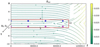 |
Fig. 1. A magnetic field topology in the vicinity of a single X-nullpoint of RCS with a thickness of 2d along the X-axis (+d and −d from X = 0) and a half width of a along the Z-axis. The particle inflows dragged in at the upper boundary (“x+”) are marked by the blue arrows and the ones at the lower boundary (“x−”) by the red arrows. The x = 0 line represents the current sheet midplane. The green lines show magnetic field lines of Bx and Bz, with the guiding field By and reconnecting electric field Ey being perpendicular to the plane of drawing. |
Particles are injected into a reconnection region from both sides of the RCS (Fig. 1). Their initial z-coordinates are uniformly distributed at z = 100 m, 200 m, 300 m,. . ., 105 m (ξx = 1 for 105 m). The distance between the injection points is Δz = 100 m. In order to study the effects of different variables qualitatively, particles are assumed to have the same initial velocity V(t = 0) = (vx0, 0, 0) perpendicular to the midplane (x = 0). In the following simulations, vx0 is chosen to be either the plasma inflow velocity (104 m s−1), or the thermal velocity (105 m s−1 for protons, or 4 × 10⁶ m s−1 for electrons).
2.2.2. Particle trajectories
Particle separation effect. The particle trajectories (Fig. 2, left col.) and energies at ejection (Fig. 2, right col.) are plotted for electrons and protons accelerated in an RCS with three magnetic field components for a current sheet thickness d = 1 m, a magnitude of magnetic field B0 = 100 G, and reconnection electric field Ey = 100 V m−1. Our simulation results confirm the previous findings (Zharkova & Gordovskyy 2004; Siversky & Zharkova 2009) that particles with opposite charges reveal strongly asymmetric trajectories and different directions of ejection into the opposite midplanes with respect to the RCS midplane. Because of their opposite charges, and the directions of gyration about By, protons and electrons become ejected into the opposite semiplanes from the midplane X = 0 (Zharkova & Gordovskyy 2004), and therefore, move in the opposite directions of the Bx (Zharkova & Gordovskyy 2004; Zharkova & Agapitov 2009). For example, in Fig. 2a, both electrons are ejected to the negative “x−” half space. On the other hand, in the same magnetic topology, protons are ejected to the positive “x+” branch.
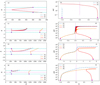 |
Fig. 2. Left panels: simulated particle trajectories on the x−z plane. Right panels: corresponding energy gains vs. the x-coordinate of the particles. Panels a and b: sampled electrons in a simulation with d = 1 m, ξy = 0.1, B0 = 100 G, Ey = 100 V m−1. Light and dark blue lines represent the transit and bounced electrons, respectively. Panels c and d: sampled protons from the same parameters as in panels a and b, respectively. Panels d and f: trajectories of protons from a different simulation with a different d = 5 m. Panels g and h: trajectories of protons in a stronger guiding field, ξy = 1.0 and d = 1 m. |
As indicated in the discussion, this separation effect was observed in the 23 July 2002 solar flare showing HXR sources spatially separated from the gamma-ray sources (Lin et al. 2003; Hurford et al. 2003), and also for the flare of 28 October 2003 (Hurford et al. 2006) and recently confirmed by laboratory experiments (Zhong et al. 2016). Furthermore, considering both the separation of electrons from ions during their crossing of the HCS and the electric field induced by this separation, polarisation electric field, which ions follow, allowed Zharkova & Khabarova (2012) to explain the asymmetry of the solar wind ion velocity during HCS crossing.
Transit and bounced particles. The particle entering an RCS at the same side from which it is to be ejected is classified as a bounced particle, while the particle entering from the side opposite to that where it is to be ejected to is classified as a transit particle (Siversky & Zharkova 2009). While travelling to the midplane, the transit particle gains energy while the bounced particle loses energy (Siversky & Zharkova 2009). This is demonstrated in Figs. 2a, b where the transit electron (labelled particle “E1” in the plot) is found to gain more energy than the bounced one (labelled particle “E2”).
Additionally, by comparing Figs. 2a–d, one can see that the transit electron gains sufficient energy and leaves the current sheet faster than the transit proton. On the other hand, the bounced electron is reflected back from RCS even before it can reach the midplane in Fig. 2a while the bounced proton can move into the midplane in Fig. 2c. The reason for this difference is that in this model the magnetic components Bx, By are large enough to magnetize the electrons, but not the protons.
Role of magnetic field components. The motion of particles of different types s (p-proton, e-electron) is associated with three characteristic frequencies related to their gyromotion about three components of magnetic field. The gyro-frequencies of rotation about Bx and By are evaluated as ωx,s ∝ ξx/ms (ωy,s ∝ ξy/ms), while the frequency f of oscillation about the Bz component is described as follows
 (5)
(5)
where  is the dimensionless electric field (Zhu & Parks 1993; Litvinenko 1996).
In Fig. 2a, the trajectories of electrons “E1” and “E2” shown at z = 300 m have ωx,e(z = 300 m) = 8.4 × 10⁵ Hz, ωy,e(z = 300 m) = 2.8 × 10⁷ Hz, and f os,e(z = 300 m) = 82 Hz. Here ωy,e ≫ ωx,e ≫ fos,e, suggesting that the electrons are strongly magnetized. In Figs. 2c and d, the selected protons “P1” and “P2” dragged in at z = 300 m have ωx,p(z = 300 m) = 460 Hz, and fos,p(z = 300 m) = 675 Hz. Both protons oscillate near the x = 0 plane for a long time because fos,p > ωx,p. Meanwhile, ωx,p(z = 1750 m) = 270 Hz is comparable with fos,p(z = 1750 m) = 285 Hz for the proton “P3” which makes the particle oscillation less obvious. Although, the inclusion of a guiding field ξy = 0.1 gives ωy,p = 1.5× 10⁴ Hz, which is much larger than fos,p, and, as result, this is not sufficient to suppress the oscillation along the acceleration path.
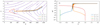 |
Fig. 3. Trajectories of selected electrons “E1” and “E2”, and protons “P1” and “P2” in Fig. 2 are plotted for the same RCS parameters as in Fig. 2 (with a guiding field By = ξB0 and ξ = 0.1); panel a: trajectories on the Z−X plane with magnetic field lines plotted in magenta as the background; panel b: energy gains by the particles vs. the x-coordinate at ejection. All the particles start from x = ± 1 m, z = 300 m. |
The trajectories of particles in an RCS with stronger By are presented for the proton “P3” in Figs. 2e and f. Now, if ωx is fixed, protons can still be magnetized leading to a change of either ωy or fos. In Fig. 2e, the half thickness d of the current sheet is increased to 5 m, for example fos,p(z = 300 m) drops to 300 Hz, which means fos,p < ωx. The oscillations of other three protons (“P4”, “P5”, and “P6”) are less obvious. This happens because ξy is increased to 1.0 in Fig. 2g, while the other parameters are the same as those in Figs. 2c and d. This results in ωy = 1.5× 10⁵ Hz, which makes ωy/fos,p even larger than the value in Fig. 2c. This leads the oscillations to have a smaller gyroradius and therefore be undetectable. In both images, the magnetized protons do not stay in the midplane for a long time, quickly gaining sufficient energy to break from the current sheet and become ejected. The bounced proton “P8” cannot even reach the midplane but instead quickly turns back and is ejected along the direction of Bz magnetic field. This trajectory is affected by a very strong guiding field By, similar to the trajectory of the electron “E1” in Fig. 2a.
In order to understand the difference between the motion of magnetized and unmagnetized particles (Zharkova et al. 2011), let us compare the trajectories of magnetized electrons “E1” and “E2” against those for unmagnetized protons “P1” and “P2” as shown in Fig. 3 for the guiding field magnitude of ξy = 0.1. In this simulation the magnitude of a guiding field By is not strong enough to magnetize protons. Therefore, they were able to cross the magnetic field lines and quickly move towards the midplane, become accelerated there and be ejected from the RCS, as shown in Fig. 3a. It is evident that the acceleration of both the transit and bounced protons happens near the midplane as shown in Fig. 3b. On the other hand, in this model the electrons become magnetized from the very beginning and as a result the bounced electrons are ejected along the local magnetic field lines. They leave the RCS too quickly so their path in the current sheet with weak guiding field is too short to be seen clearly in the same picture with protons. The transit electrons on the other hand move towards the midplane, pass through it, and leave the RCS following the magnetic field lines, as shown in Fig. 3a. Therefore, there are no oscillations of electrons recorded near the midplane for the magnetic topology with a weaker guiding field.
2.2.3. Analytical estimations of particle energy gains
Because Bx is a function of z, the energy gains by particles injected at different positions are expected to be different. It was shown that the maximum energy gain of an unmagnetized particle in the RCS with ξy = 0 (in the absence of guiding field) can be analytically evaluated (Speiser 1965; hereafter S65) as
 (6)
(6)
where ms is the mass of the particle of type s (p-protons, e-electrons).
Further investigation of particle trajectories in a reconnecting current sheet with a fixed perpendicular magnetic component Bx demonstrates the effect of the addition of a small guiding field By (Martin et al. 1994; Zhu & Parks 1993, etc). Litvinenko & Somov (1993) and Litvinenko (1996) showed that the particles gain much higher energy in the magnetic topology with the non-zero guiding field with the ratio  . By assuming that a test particle starts acceleration at the midplane (x = 0) and ignoring how the particle arrives into the midplane, the energy upon ejection of the magnetized particles was estimated (Litvinenko 1996; hereafter L96) as:
 (7)
(7)
when Bx is fixed.
Siversky & Zharkova (2009) studied the electron acceleration in an RCS with test particle approach for a magnetic topology similar to Eq. (1), while considering Bx(=−Bz0ξx0) not to be a function of z-coordinate. They found that the energy gains by the transit electrons agree with Eq. (6), if Bx and By are too weak to magnetize the electrons, and with Eq. (7) for magnetized electrons if Bx and By are strong. At the same time, the energy gains by the bounced electrons agree with Eq. (6) only for arbitrary Bx and By.
In the current paper, the parameters derived by Siversky & Zharkova (2009) for proton acceleration are probed by the results presented in Fig. 4. The physical parameters inside the RCS are the same as in the original paper (Siversky & Zharkova 2009), Bz0 = 10 −3T, Ey = 250 V m−1, and d = 1 m. The energies of ejected protons are shown to be close to the analytical estimations above in both the unmagnetized and magnetized limits, which agree with the findings of Siversky & Zharkova (2009). Additionally, the simulations of proton motion show that the switch from unmagnetized to magnetized regions happens at magnitudes of Bx ∼ 2× 10⁻³T, higher than for electrons in the transit branch when By0 ≡ 10−4 T in Fig. 4a. On the other hand, for the same By0 as reported by Siversky & Zharkova (2009), this transformation for electrons occurs at Bx ∼ 10 −5T, that is, smaller than for protons. Meanwhile, for a fixed Bx0 ≡ 10−3T, the switch from unmagnetized to magnetized protons happens at the guiding field of By ∼ 2× 10⁻³T as shown in Fig. 4b. The similar switch from unmagnetized to magnetized electrons occurs at By ∼ 6 × 10⁻⁵T, which is much smaller than the one for the protons for the same Bx0. Thus, we conclude from Fig. 4 that much stronger magnitudes of magnetic components Bx (By) are required to magnetize protons than for electrons.
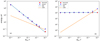 |
Fig. 4. Panel a: energies of ejected protons vs. different Bx for fixed By0 ≡ 10−4T. Panel b: energies of ejected protons vs. different By with Bx0 ≡ 10−3 T. The energy gains from Eqs. (6) and (7) are plotted in blue and orange solid lines. The other parameters are Bz0 = 10 −3T, Ey = 250 V m−1, d = 1 m. |
2.2.4. The simulated energy gains
Electron energy gains. The simulated energies gained by electrons at ejection from a current sheet are shown in the upper panel of Fig. 5. The magnetic topology is described by Eq. (1) with B0 = 0.01T, E = 100 V m−1, ξy = 0.1, d = 1 m, and a = 105 m. The initial velocity vx,0 is assumed equal to 104 m s−1 (see Fig. 5a), which is much smaller than the electron thermal velocity in the corona, while in Fig. 5b, we adopt the thermal velocity of coronal electrons, vx,0 = 4 × 10⁶ m s−1, discussed in Sect. 2.2.1.
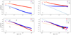 |
Fig. 5. Energy gains (in keV) by electrons and protons at the end of simulation vs. their initial positions ξx (t = 0). The blue triangles represent the particles starting at x = −1 m and the red dots are the ones beginning at x = 1 m. For electrons: panel a: initial velocity vx(t = 0) = 104 m s−1, panel b: vx(t = 0) = 4 × 10⁶ m s−1. For protons: panel c: vx(t = 0) = 104 m s−1, panel d: vx(t = 0) = 105 m s−1. Also, there are protons in the transit group coming back to the lower boundary, and protons in the bounced group that cross the RCS in the ξx > 0.2 region; these are marked by the green stars and purple plus symbols, respectively. The estimated maximum energy gains from Eqs. (6) and (7) are again plotted in solid blue and orange lines. The injecting ξx- coordinates of the selected electrons and protons in Fig. 2 are also marked in panels a and c. The electromagnetic fields are described in Sect. 2.1.1: B0 = 0.01T, E = 100 Vm s−1, ξy = 0.1, d = 1 m. |
The energy gained by the transit and bounced particles are very different as seen in the spectra presented in Fig. 5a and b. The simulation results shown in Fig. 5a of the energy gains by bounced and transit electrons match rather closely the analytical estimations described by Eqs. (6) and (7), respectively. This suggests that the energy distributions of ejected electrons comprise two populations of electrons, transit and bounced, and, thus, are expected to have distributions with double maxima, as was shown earlier by Siversky & Zharkova (2009).
In the “x−” branch of Fig. 5b, only the electrons, which are very close to the X-nullpoint, become accelerated because in a strong Bx region far away from the X-nullpoint their original thermal energy is larger than the maximal energy gains at a given location as estimated by Eq. (6). As a result, the electrons of the ξx > 0.01 part in the “x−” branch are not accelerated and keep the original thermal energy. The final energy gain of the bounced electrons in this region is not related to ξx. We note that the energies gained by the transit electrons in the topologies with a weak guiding field, for example, ξx (t = 0) = 10−3 and 2 × 10⁻³, are below the estimations from Eq. (7) as shown in Figs. 5a and b. In these simulations, the particles actually move to the half space with z < 0 before they reach the midplane and subsequently become bounced electrons. This pattern is explained in Sect. 2.2.5.
Proton energy gains. In the same magnetic field topology, protons trajectories and energy gains are very different from those of electrons as shown in the bottom panel of Fig. 5. Unlike the electrons, the most energized protons (≳ 1 keV) correspond to those described by Eq. (6), and not Eq. (7). While the ejection energies of less energized protons (≲ 0.1 keV) are close to the magnitudes estimated from Eq. (7). Technically, this means that if Ey0 and Bz0 are fixed, in thicker current sheets (d ≫ 1 m) in the ξx < 0.1 region, protons would gain higher energy with magnitudes close to Eq. (7). On the other hand, in the ξx > 0.2 region of Fig. 5b, the energy gains are smaller than the initial thermal energies of the protons. Hence, in this “no acceleration” region, there is no clear relation between ξx and ΔE.
We note that in the ξx < 0.01 region, the protons gain less energy than the corresponding ΔES65 with the same Bx. One important fact in our simulations is that Bx is not a fixed value. It changes in RCS with z-coordinate as expressed in formula (1). Consequently, these most accelerated protons move through the region with increasing Bx when they travel a long distance in the +z direction. Subsequently, energies of ejected protons calculated for Bx(t = 0) in Fig. 5c and d become smaller than the energy gained by the particles entered from x = −1 m (blue line).
2.2.5. Particle drifts in RCS of different thickness
As shown in Fig. 2, when a current sheet becomes thicker, the transit proton will first rotate toward the X-nullpoint due to the gyromotion about By, while the bounced proton directly rotates further away from the X-nullpoint. A similar difference between the transit and bounced electrons is also presented in Fig. 3a. This effect can be explained by using the estimation from Litvinenko (1996) (Eq. 27). To simplify the calculations, let us change the magnetic field topology to:
 (8)
(8)
where Bx is considered to be a fixed value across the whole domain for this part, and ξx,0 and ξy,0 are the ratios of transverse and longitudinal magnetic fields to the tangential component B0. Now we produce a simple estimation to show how far the transit particles can move towards the X-nullpoint. By assuming that the acceleration in the −z direction comes from the gyromotion about By, the particle motion is described by the equation
 (9)
(9)
Subsequently, by ignoring the −vy × Bx term in the early stage of acceleration in the RCS, and by assuming vx to be dominated by the Ey × Bz drift, one obtains
 (10)
(10)
By integrating this equation, the travel time for the transit particle to arrive to the midplane from the injection boundary at x(t = 0) = −d is estimated as follows.
 (11)
(11)
If we assume that the particle keeps moving in the semiplane along −z before it reaches the midplane (X = 0), then the estimation gives us
 (12)
(12)
On the other hand, the zero-order solution from the multi-scales analysis (Litvinenko 1996) gives the particle trajectory in the above magnetic topology as follows.
 (13)
(13)
where the length scale is scaled in d, and the timescale is in a gyroperiod Ω−1 = mc/eB. In these new units, the initial position for the transit particle is defined as  . Hence, we find that the particle first moves to a minimum ΔzL < 0 before it starts to travel along +z to infinity (or into loop legs).
Let us test these estimations, Δze and ΔzL, for the current sheets with a different thickness of d = 1m,. . ., 40m for the parameters B0 = 100 G, ξx = 0.006, ξy = 0.1, E = 100 V m−1. In each simulation, let us measure the travel time for a particle to reach the midplane Δts and the travel distance along the z-axis towards the X-nullpoint Δzs. The comparison of the simulations, the simple estimations (Δte, Δze), and the minimum value of Z for t ≥ 0 from Eq. (13) are presented in Table 1. In summary, the estimation calculated above gives the right order of magnitude for both parameters Δts and Δzs. When d is larger, the difference between Δze and Δzs becomes larger. This is because the estimation assumes the particle to keep going towards the X-nullpoint before it reaches the midplane. In fact, the acceleration in the z+ direction would start pushing the particle to run away from the X-nullpoint before reaching the midplane. On the other hand, the approximation given by Eq. (13) underestimates this drift.
Comparison of different times and magnitudes of Δz for RCSs with different thickness.
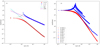 |
Fig. 6. Final energy gains (in keV) of the protons plotted vs. ξx at their initial positions (see Sect. 2.1.1 for more details). Panel a: for RCS with d = 40 m. Panel b: For RCS with different thickness: d = 1 m, 10 m, 40 m, 80 m, 100 m. The “x+, x+”/“x+, x−” and “x−, x+”/“x−, x−” are using the same markers to keep the picture visually clear. Equations (6) and (7) for different d are not plotted in panel b for the same reason. The other parameters are the same as described in Sect. 2.1.1: B0 = 0.01T, E = 100 V m−1, ξy = 0.1. |
This initial drift towards the X-nullpoint has two effects on transit particle acceleration in the RCS: (a) it gains more energy, according to Eqs. (6) and (7) because the transit particle moves closer to the X-nullpoint where the local Bx is smaller, and (b) if the particle hits the z = 0 boundary before it changes direction, it will go to the other half space z < 0 where it will become a bounced particle. Therefore, we suggest that there is a special “non-transit” area in the RCS. If the distance −z between the X-nullpoint and the injection point of the particle is too short, the particles all become bounced. In order to demonstrate this phenomenon, the half thickness of current sheet d is increased to 40 m.
The simulated energy gains by the protons are presented in Fig. 6a, clearly showing the transformation from the bounced to transit on the “x−” side of the RCS, which is not present in the d = 1 m case in Fig. 5. The most accelerated particles do not enter the RCS very close to the X-nullpoint but at some short distance from the X-nullpoint in Fig. 6a. In this “non-transit” region where Bx is small, Eq. (6) is no longer valid. Besides, the gained energy of the transit particles in the “x−” branch is higher than both Eqs. (6) and (7) in the ξx ∈ (10−2, 3× 10⁻²) region, while the bounced particles in the “x−” branch have less energy where By is relatively strong. We believe this is also due to the drift of particles towards the X-nullpoint.
Furthermore, we simulated particle trajectories and energy gains in the current sheet with different thickness of d = 10 m, 40 m, 80 m, 100 m for the configuration similar to Fig. 5. All the particles are initialized at low energies as shown in Fig. 5a, meaning that we can clearly detect the acceleration even if ξx is very large. The results show that if the half thickness d increases, the transformation points between the transit and bounced particles in the “x−” branches are moving further away from the X-nullpoint, as is expected (see Table 1). At these peaks, the energy gained by protons increases if the current sheet becomes thicker. It is shown that in these simulations the energy of ejected protons is eight times larger than the estimated energy gains by Eq. (7) for the same ξx in Fig. 5b.
3. Particle acceleration in multiple O- and X- nullponts
As indicated in the Introduction, large current sheets are often found broken by tearing instability into smaller magnetic islands. These were first predicted by 2D PIC simulations (Drake et al. 2006a) and later observed in various events: flares (Lin et al. 2005; Oka et al. 2010; Bárta et al. 2011; Takasao et al. 2012; Nishizuka et al. 2015), the current sheet associated with CMEs (Song et al. 2012), and the magnetotail (Oieroset et al. 2002; Zong et al. 2004; Chen et al. 2008; Wang et al. 2016). The magnetic islands are found to have different shapes either merging into each other (coalescent islands) (Kliem 1994; Song et al. 2012) or becoming squashed in one direction (Drake et al. 2006a). This change of island topologies can essentially modify the particle acceleration scenario in an RCS with magnetic islands.
In this section, particle acceleration is considered in 3D current sheets with magnetic islands. This allows us to probe the applicability of the concepts of preferential ejection, transit versus bounced particles, and unmagnetized versus magnetized particles in the magnetic topologies with magnetic islands. We can also compare energy distributions of particles of the same charge entering current sheets from the opposite sides (transit and bounced particles) and decipher whether or not the difference in their drift velocities is still sufficient for the production of turbulence as as it was in a standard RCS with a single X-nullpoint (Siversky & Zharkova 2009).
3.1. Magnetic and electric field topologies
3.1.1. Magnetic field in islands
Let us consider current sheets with a few 3D O-nullpoints separated by X-nullpoints from both sides of magnetic islands, which are initially assumed to have the same shapes and dimensions. The magnetic field in the islands is adopted from Kliem (1994), which is also known as the Fadeev equilibrium model (Fadeev et al. 1965) with added constant out-of-plane guiding field:
 (14)
(14)
 (15)
(15)
 (16)
(16)
where d is again the half thickness of RCS near the O-nullpoint, ξ is the same parameter as in Eq. (1), and ϵ, k are the mathematical parameters controlling the dimension of the periodic islands: k = Li/d measures the ratio of the distance Li from the centre of the O-nullpoint to the closest X-nullpoint, also referred to as the half length of the island, to the current sheet half thickness di. This model is valid for a series of identical islands periodically occurring along the x = 0 m plane. In our simulations, k =1.0, 0.03125 is used, where k = 1 is the original value accepted in Kliem (1994) and is also used in the continued test particle study of Li & Lin (2012), and k ≈ 0.03125 for the magnetic geometry in Drake et al. (2006a). Meanwhile, ϵ = 0.3 to remain consistent with Kliem (1994).
We have to emphasise that Fadeev’s model represents a chain of infinite number of highly identical magnetic islands in the RCS. We consider particles to be uniformly distributed at both boundaries of the chain and injected into these islands, deriving their trajectories and energy distributions. In reality, there could be only a few, or even just a single magnetic island inside the RCS, and these islands are not necessarily as symmetric as in the model we adopted. Hence, any evaluation of the energy spectra of accelerated particles in this model has its natural limitations, which need to be kept in mind, before comparing the simulated spectra with observations.
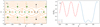 |
Fig. 7. Panel a: plasma inflow (green arrows) and outflow (black arrows) directions in a magnetic islands chain. The solid orange lines show the magnetic field in the x−z plane. Here islands “1” and “2” represent the squashed islands, while islands “3” and “4” represent the coalescent islands. Panel b: red dash-dot line shows the Ey from squashed islands on the midplane from Eq. (17). The blue dash line shows the Ey from coalescent islands on the midplane from Eq. (18). Here k = 0.03125. |
3.1.2. Reconnection electric field
An important component determining particle acceleration in the RCS is the reconnection electric field, which is determined by the local plasma inflow velocity and the gradient of the magnetic field. (see Eq. (2)). It is evident that the Ey would reverse its sign if the local plasma velocity changed direction. Therefore, we introduce two types of magnetic island: one has plasma inflows at both X-nullpoints of the magnetic island, and the other one has plasma pushed away at certain X-nullpoints.
Squashed magnetic islands. For this type of magnetic island, which has eclipse-type shapes, the plasma is suggested to be moving into an O-nullpoint from both X-nullpoints. This motion is similar to the plasma inflow coming into the RCS as shown by the green arrows in Fig. 7a. The corresponding electric field in such islands is adopted from Li & Lin (2012):
![Mathematical equation: $ \begin{equation} E_y = E_{y0} [0.6 + 0.4 \cos(k z/d)]. \label{eq:ESPSUNDSCRos} \end{equation} $](/articles/aa/full_html/2018/12/aa33599-18/aa33599-18-eq21.gif) (17)
(17)
This means that the plasma flows into the squashed islands from all directions, which makes Ey parallel to the reconnection electric field everywhere. Therefore, the particles in squashed islands are only affected by Ey > 0 as shown by the red line in Fig. 7b.
Coalescent magnetic islands. In contrast, the electric field for coalescent islands where the two islands move towards one another is suggested by Kliem (1994) as
 (18)
(18)
This electric field is not symmetric about the centre of the island. Although this type of magnetic island could have the same dimensions as the squashed one, the direction of the plasma flow at certain regions is different. As shown by the black arrows in Fig. 7a, the coalescent structure described by Eq. (18) means that two islands (e.g. islands “3” and “4”), one on each side of the X-nullpoint, are merging into a single one. In this case, the magnetic islands centred at z = 64 m and 192 m are moving towards one another (shown by horizontal black arrows) and merging into a single island. The plasma between the islands is therefore pushed outwards as shown by the vertical black arrows. In this contracting (outflow) region, the electric field Ey < 0 is anti-parallel to the reconnection electric field at the boundary as shown in Fig. 7b. Hence the coalescent islands described by Eq. (18) actually contain both a contracting region (with outflow, Ey < 0) and a squeezing region (with inflow, Ey > 0), while the squashed islands only have Ey > 0.
Now, in order to match with our previous studies near the X-nullpoints, the simulations would start with the parameters close to the corona environment: n = 1015 m−3, d = 2 m, T = 100 eV, E0 = 100 V m−1, B0 ≈ 102 G and ϵ = 0.3, leaving k as a free parameter.
3.2. Simulation results
3.2.1. Particle trajectories in the magnetic islands
Let us use k = 0.03125, set to match the dimension of the islands in Drake et al. (2006a), and apply to our RCS model. On the other hand, the electric field of coalescent islands following Eq. (18), Figs. 8a–d, and the electric field of squashed islands following Eq. (17), Fig. 8e. The trajectories and energy gains of electrons in these islands are shown in the left and right columns of Fig. 8.
Similar to the single X-nullpoint shown in Fig. 2, in the multiple O-nullpoints an unmagnetized electron moves away from the X-line and crosses the magnetic field lines along the midplane (x = 0) as shown in Fig. 8b. On the other hand, if the particle is magnetized, it circles inside the O-nullpoint following the magnetic field lines as shown in Fig. 8a. The trajectory of the magnetized electron is similar to those reported in other studies (Kliem 1994; Drake et al. 2006a; Li & Lin 2012; Dahlin et al. 2015). In both cases, magnetized or unmagnetized, accelerated electrons go back and forth inside a magnetic island between the two X-nullpoints. The acceleration mechanism here is identical to the previous studies in the RCS with a single X-nullpoint occurring due to the out-of-plane reconnection electric field. Naturally, following Eq. (6) the energy gained by particles is larger when Bx is weaker if the other parameters are identical.
Similar to an RCS with a single X-nullpoint, the presence of a guiding field By in the O-type reconnection region leads to particles gaining more energy than without guiding field (see Stanier et al. 2017, for details, and references therein). For the simulation time of  (
( s) there are three different cases presented: no guiding field (Fig. 8a), weak guiding field (Fig. 8c), and strong guiding field (Fig. 8d). During this limited time, the electron accelerated in the topology with the strongest guiding field very quickly gains sufficient energy to escape from the very first island, within which it was trapped. If the guiding field is weaker, the electrons are found trapped in the first island much longer and their acceleration is much slower, meaning that it would take a longer time for particles to gain enough energy to escape the island (Fig. 8c). If the guiding field is zero, the trapping time for the electron is even longer.
Energy gains by particles in coalescent and squashed islands are also different. The electric field in coalescent islands (see Eq. (18)) shown in Fig. 8a between 0 and 240 m has a squeezing region with Ey < 0 at z ∈ (0, 50 m) and a contracting region where Ey < 0 as shown by the blue dashed line in Fig. 7b at z ∈ (80 m, 120 m) and at z ∈ (120 m, 180 m), while the two islands are moving towards each other. The electron is shown in Fig. 8a to gain energy only in the squeezing region.
On the other hand, the electric field of a squashed magnetic island in Fig. 8e, which is described by Eq. (17), has two squeezing regions (Ey > 0) located near z = −120 m and 0 m as shown as the red dash-dot line in Fig. 7b. Therefore, the electrons become accelerated at both X-nullpoints of the island, which, during the same simulation running time, results in the particle gaining more energy in this island compared to the coalescent one (Fig. 8a).
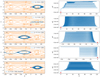 |
Fig. 8. Test-particle orbits (left col.) and energy gains (right col.) vs. z-coordinate (blue lines), obtained during the same running simulation time, Δt = 8×10⁻⁵ s for: panel a: magnetized electron in the magnetic island described by Eqs. (14) and (16) with B0 = 100 G and the guiding field By = 0; panel b: unmagnetized electron in the magnetic island with the same dimension as panel a and B0 = 10 G; panel c: magnetized electron in the magnetic island which has the same Bx and Bz components as panel a with added guiding field By = Bz0 ξ, where ξy = 0.1; panel d: magnetized electron in the magnetic island which has the same Bx and Bz components as panels a and c but with a stronger guiding field, ξy = 1.0; and panel e: electron in the magnetic island which has the same magnetic field topology as panel a for the electric field following Eq. (17) representing squashed islands. The magnetic field lines of Bx, Bz are plotted in orange lines for all cases. Here k = 0.03125, ϵ = 0.3. |
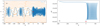 |
Fig. 9. Simulation result for a strong reconnection electric field Ey0 = 690 V m−1. Panel a: electron trajectory in the X−Z plane. The orange lines present the magnetic field in this plane. Panel b: energy gained by the electron vs. z-coordinate. The other parameters are identical to Fig. 8a: k = 0.03125, ϵ = 0.3, ξy = 0, B0 = 100 G. |
By comparing the results above with those for electron acceleration in a single X-nullpoint, it can be found that the travelling distance of accelerated particles along the midplane is much shorter in the multiple X- and O-nullpoints (as shown in Fig. 2). For example, in highly magnetized cases, the particle would either be trapped in multiple magnetic islands and become accelerated again and again (e.g. Fig. 10c), or be trapped within a single island until it reached a very high energy allowing it to break from an RCS. While the particles still gain energy when they move close to the other X-nullpoints, very often the first trapping island can be sufficient for electrons to gain sub-relativistic energy and to break from an RCS. This effect significantly reduces the restrictions on a current sheet length required to produce high-energy (relativistic) electrons, thus, making current sheets with magnetic islands the efficient primary accelerators of particles.
A typical simulation of strong particle acceleration within a single coalescent island is presented in Fig. 9a. As mentioned in Sect. 2.2.2. in the RCS with a single X-nullpoint, increasing Ey means that the gyrofrequency  about the magnetic component Bx becomes relatively smaller than fos from Eq. (5) about the Bz component. The trajectory of the electron in Fig. 9a corresponds to the unmagnetized case. In this simulation, the energy gained by the electron reached ≃ 2 × 10⁶ eV (e.g., Fig. 9b) in a single magnetic island of length ≈ 126 m within the timescale of
  . Furthermore, once the electron had left the first island, the highly energetic particle actually spent more time near the X-nullpoints rather than circling into the other islands as presented in Fig. 9. This process forms the electron clouds about the X-nullpoints, which is similar to that reported by Pritchett (2008) using particle-in-cell approach.
3.2.2. Preferential ejection of particles with opposite charges
Let us check how the particles with opposite charges leave the RCS with magnetic islands and whether or not they are ejected to opposite semiplanes from the RCS midplane.
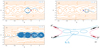 |
Fig. 10. Trajectories of an electron (panel a) and a proton (panel b) accelerated in similar magnetic islands. Panel c: Trajectory of an electron in the edge island as described by Eq. (20), which has an open field topology edge at |z| > 10. d = 2 m, ϵ = 0.3, k0 = 1.0, ξy = 1. The sampled particles are all initialized at x = 0, z = 0 to reduce the computing time for the particle motion from the RCS boundaries. The orange lines present the magnetic field in the X−Z plane. Panel d: example of preferential ejection of electrons and protons from an RCS with multiple X-nullpoints. |
In order to include in the study an open field on the edge of a current sheet with islands, allowing us to show how a particle can leave a chain of magnetic islands, the following modification is applied to the coalescent model. The magnetic components are described by Eqs. (14) and (16), and the electric field Ey by Eq. (18), with k to be selected as follows:
 (19)
(19)
where ϵ = 0.3 and k0 = 1.0. This change increases the length Li of the islands beyond |z| > 8.
Furthermore, the magnetic component Bx is replaced by
 (20)
(20)
Together these changes introduce an open field topology attached to a magnetic island chain near |z| = 8 as shown in Fig. 10c, where the guiding field ξy = 1 is kept the same as in Fig. 10a.
The acceleration paths of electrons and protons in a chain of magnetic islands are presented in Figs. 10a–c, where a strong guiding field By ≡ Bz0 uniformly penetrates through the whole simulation domain. One can see that the electrons cross the X-nullpoint while rotating clockwise, whereas the protons rotate anti-clockwise; they are therefore ejected from a current sheet into opposite semiplanes from the middle plane. Both electrons and protons move to the “preferential direction” as demonstrated in Fig. 10d, where ϵ = 0.3, k = 1.0.
The new simulation shows that when the electron moves to the open field region, it still moves to the preferential semiplane as demonstrated in Fig. 10d. This verifies that, in the presence of a strong guiding field there is always asymmetric ejection of electrons and protons with respect to the RCS midplane, regardless of whether magnetic islands are present or not.
Therefore, in the RCS with multiple X- and O- nullpoints, the accelerated particles maintain preferential ejections despite being trapped in the islands and circling around the O-points, which was also confirmed by other authors (Kliem 1994; Drake et al. 2006a).
Besides, we note that the particles are not escaping or being ejected from O-nullpoints perpendicular to the midplane of magnetic islands. In fact, the particles are shown only to leave the island near the X-nullpoint either moving to the next island, or following the open field lines to leave the whole current sheet. In all cases, the ejection direction when the particle leaves a current island is defined by the magnetic and electric field signs and the particle charge.
3.2.3. The effect of the initial position: transit and bounced particles
In an RCS with a single X-nullpoint, the distance z from the X-nullpoint and the side from which the particle enters the RCS, for example, whether the particle is transit or bounced, will effect the final energy gained by these two types of particle. Because bounced particles enter from the side from which they will later be ejected, they are decelerated and repelled away before they reach the midplane and become accelerated by a reconnection electric field. While the transit particles, which enter from the opposite side, will continue to gain energy until they are ejected from the RCS. Similar phenomena are expected during the particle acceleration in O-nullpoints.
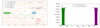 |
Fig. 11. Left panel: different trajectories of electrons in coalescent islands for particles, which are moving away (brown and red colours) because of the contracting electric field Ey; for a “transit” electron (magenta line) moving slowly towards the midplane x = 0 for ξy = 1; for a “bounced” particle (the purple line), which takes a longer time to move into the island than for the “transit” one. The red dots represent the original positions. The magnetic field lines in x−z plane are plotted in orange. In z > 0 region, the contracting Ey < 0 area is indicated between the second and third (aqua coloured) dash lines. Right panel: energy gains versus z-coordinate of the selected “transit” and “bounced” electrons, entering the RCS at x0 = ± 2 m, z0 = 28 m. |
The particle trajectories obtained for coalescent islands for different initial positions are demonstrated in Fig. 11. By comparing these trajectories with those plotted in Fig. 10d, one can identify that transit electrons enter the RCS from the x < 0 side in the z ∈ (0, 64 m) region, and from the x > 0 side in the z ∈ (64 m, 128 m) region because now Ey < 0. The bounced electrons enter from the opposite side of an RCS in these two regions. However, the contracting electric field of coalescent islands Ey (< 0) is pushing particles, both transit and bounced, away from the RCS (the brown and red lines in Fig. 11); as a result, they do not become strongly accelerated. On the other hand, in multiple coalescent islands it is more difficult for the bounced particles (shown with the purple and brown lines in Fig. 11) to move into the acceleration region of islands than for the transit ones (shown by the green line in Fig. 11) in the squeezing region where Ey > 0.
Furthermore, a guiding field By is well known to enhance the energy gain by particles in the RCS. However, in some cases, a strong guiding field would magnetize these particles before they move into the islands, and they are forced to move quasi-parallel to the field lines in the X−Z plane at the boundary (the magenta line in Fig. 11), which prevents the particles at the boundary from moving into the island, similar to observations (Zharkova & Khabarova 2012).
Once the ambient plasma particle enters an island in the RCS, it circles multiple times inside it and leaves the island only when it reaches the energy sufficient to break from the given magnetic field topology. The final energy of ejected particles is measured when they leave the first trapped island. Since the horizontal and vertical sizes of islands considered in this model are rather small, this cycling inside the islands nearly equalizes the energy gains by the transit and bounced particles (see Fig. 11b for transit (green line) and bounced (purple line) electrons). This happens because the trapping stage, when the bounced particle loses its energy while reaching the midplane, is too short compared to the acceleration path inside the island. As a result, there is a small difference between the energy gains of transit and bounced particles (compare the green and magenta lines for energy gains), which is hard to observe for the shorter islands shown in Fig. 11.
The difference between transit and bounced particles can be easier to observe within a single island in the case when particles are weakly magnetized as shown in Fig. 12a. Here, in order to compare with the electron trajectory in the RCS with a single X-nullpoint as presented in Fig. 2a, we accepted k = 0.003125 so that the distance between the injection point and the closest X-nullpoint is again 300 m, and ξy = 0.1 to ensure both particles could drift into the same island. We found that within the selected longer magnetic island there is a difference of eight magnitudes between the energy gains of the transit and bounced particles (compare the energy gains for transit (blue line) and bounced (magenta line) particles in Fig. 12b).
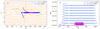 |
Fig. 12. Panel a: different trajectories of a pair of selected transit (blue line) and bounced (purple line) electrons in a coalescent island. They enter the RCS at x0 = ± 2 m, z0 = 300 m. The magnetic field lines in the x−z plane are plotted in orange. Panel b: corresponding energy gains vs. z-coordinate of the two particles in panel a. The parameters for the simulated magnetic islands are k = 0.003125, ϵ = 0.1, B0 = 10G, ξy = 0.1. |
3.2.4. Energy gains
Particle energy gains in a 3D current sheet with a single X-nullpoint discussed in Sects. 2.2.3 and 2.2.4 are mainly effected by a reconnection electric field Ey and the particle gyration about all three components of magnetic field. These parameters define how long the particle will be trapped inside a given magnetic field topology and thus accelerated by this electric field. In multiple magnetic islands there are additional parameters affecting the particle trajectories, such as k defined in Eq. (16) for example. Let us explore the effects of these parameters on particle energy gains in the models with magnetic islands considered above.
Firstly, it is found that when the guiding field is stronger, a particle spends more time cycling in the island before it gains sufficient energy to escape the trapped island described in Sect. 3.2.1. These energy thresholds of the ejected electrons are measured when the particles leave the first islands as shown in Fig. 13a. For this type of magnetic topology, the energy gain ΔE_es is roughly proportional to a guiding field magnitude, for example,  . This dependence is not as strong as for the X-nullpoint-type acceleration defined by Eq. (7), suggesting that the electrons in these simulations are not fully magnetized.
Secondly, by increasing the length of the magnetic island Li, we discovered that the larger a magnetic island is, the higher the energy gained by the accelerated particles as shown in Fig. 13b. This is because near the X-nullpoint the amplitude of the fluctuation of Bx(z) is smaller, while the amplitude of Ey drops slower when Li/d is larger, as shown in Fig. 13c and d. It was shown by Zharkova & Gordovskyy (2005a) that in the X-nullpoint acceleration, the increase of Ey/Bx would strongly enhance the energy gain. By decreasing k in Fadeev’s model (Eq. (16)), Li could be elongated in the midplane. Therefore, the energy gains of particles at ejection from the first island increase when the ratio Li/d of the island is larger, even when Bz0, Ey0, and d are the same outside of the RCS, as presented in Fig. 13b.
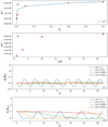 |
Fig. 13. Panel a: energy gains by the escaping electrons (measured when they leave the first trapped island) vs. the guiding field magnitude: ξy = 0.0, 10−4, 10−2, 0.1, 0.6, 1.0. The other parameters are: Ey0 = 100 V m−1, Bz0 = 100G, ϵ = 0.3, d = 2 m, k = 0.03125. Panel b: energy gains by the escaping electrons vs. the half length of the islands: Li = 2 m, 6.4 m, 20 m, 64 m. Panel c: fluctuation of Bx on the x = 0 m plane for different aspect ratios Li/d (k−1). Panel d: corresponding fluctuation of Ey on the x = 0 plane. The other parameters are: Ey0 = 100 V m−1, Bz0 = 100G, ξy = 1.0, ϵ = 0.3, d = 2 m. |
Finally, a broader scan of the particle energy gains for different magnitudes of Ey for both “coalescent” and “squashed” islands is shown in Fig. 14. The energy ΔE gained by the electron near the first X-nullpoint is proportinal to  in Fig. 14a, and the energy gains increase linearly with the growth of the electric field of the island. On the other hand, maximum energy gains by the electrons in the first islands presented in Fig. 14b are also dependent on a guiding field (Zharkova & Gordovskyy 2005a; Pritchett 2008).
When By = 0, the energy gained by electrons ΔE is proportional to  for the squeezing electric field and
  for the contracting electric field. Additionally, when By is strong,
  for the both structures. This suggests that the squeezing electric field is much more efficient on particle acceleration in a magnetic island. This relation is also applicable in Eq. (7) for the magnetized particle acceleration in an RCS with a single X-nullpoint. However, it is evident that for any guiding field the particle dragged from the boundary into the island becomes strongly accelerated by a squeezing electric field in the very first X-nullpoint, similar to Fig. 3.
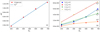 |
Fig. 14. Panel a: energy gains vs. reconnection electric field Ey for electrons at ejection from the first X-nullpoint. Panel b: energy gains vs. reconnection electric field Ey for particles ejected from the first trapping coalescence (C) and squashed (S) islands. |
The simulated energy spectra of accelerated electrons gained in the considered RCS (with or without the constant guiding field By) are plotted in Fig. 15 for the two magnitudes of magnetic field: 10 G and 100 G. We use 106 particles with the initial Maxwellian distribution corresponding to a solar coronal temperature of 2 × 10⁶ K. Initially, particles are distributed uniformly and randomly injected into the region x ∈ [−10 m, 10 m], z ∈ [0, 256 m], which covers two pairs of coalescent islands in this RCS. The initial velocities of injected particles are pulled out from a thermal distribution using the Monte-Carlo method.
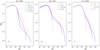 |
Fig. 15. Energy spectra of electrons accelerated during t = 8 × 10⁻⁵ s in the coalescent islands with magnetic field magnitudes: panel a: B0 = 100 G, and panel b: B0 = 10 G: Both ξy = 0 (the blue dash-dotted line) and ξy = 1 (red lines) cases are compared in the same plot. Panel c: energy spectrum of electrons in squashed (“S”) islands (blue dash-dotted line) with ξy = 0. For comparison, the spectrum of the ξy = 0 case in panel a from coalescent islands (“C”) is also plotted as a background. The green dotted lines indicate the initial thermal distribution with T0 = 100 eV. The other parameters are as follows: Ey0 = 100 V m−1, ϵ = 0.3, k = 0.03125, d = 2 m. We note that the dashed lines show only the referral power-law indexes in different cases and do not represent the whole fitting range of energies gained (up to three orders of magnitude on the plot). |
It is evident that in a given magnetic field topology the energy spectra of accelerated electrons form high-energy power-law tails from the initial Maxwellian (thermal) spectrum with EeV > 500 eV as shown in Fig. 15. Fitting a power-law spectrum E −p to the higher-energy spectra simulated for the magnetic field magnitude of B0 = 100 G shown in Fig. 15 shows a spectral index p = 2.4 for electron energies EeV in the range 5 × 10² − 104 eV. The spectral index of the simulated spectrum is similar to the test particle results reported by Li & Lin (2012), and slightly smaller than the results obtained from the 2D PIC simulation by Oka et al. (2010). In magnetic topologies with a strong guiding field (the blue dash-dot line), the electrons are shown to be accelerated to higher energies of 104 or a few units of 105 eV, expanding the high-energy tail to 2 × 10³ − 4 × 10⁵ eV. The spectral index of electrons in this range becomes smaller approaching p = 1.2, similar to those reported by Guo et al. (2014). In general, we can deduce that the ranges of electron energy gains and spectral indices in magnetic islands of different shapes and dynamics discussed in several paragraphs above show a relatively good fit to the parameters of HXR spectra observed in solar flares with the RHESSI payload (Holman et al. 2011).
The harder spectrum for electrons accelerated in the magnetic topology with a strong guiding field suggests that, similarly to a single X-nullpoint, electrons in the islands are accelerated much more efficiently than without a guiding field. For a weaker magnetic field magnitude B0 = 10 G, the spectral index of the higher-energy tail becomes smaller, p = 1.13 for ξy = 1, while remaining about p = 2.0 for a weaker guiding field, ξy = 0. The energy spectrum plot in Fig. 15b demonstrates that for the case of a strong guiding field there are more electrons with high energies E > 105 eV, making the spectrum harder. The drops of energy spectra seen at the highest energies are likely to be caused by the smaller number of particles with very high energies. Similar drops are often reported in the HXR photon spectra from the RHESSI data (Holman et al. 2011), which are also attributed to the same reason of smaller statistics of HXR photons at higher energies.
On the other hand, in Sect. 3.2.1 particles are shown to be accelerated to greater energies in squashed islands than in regular islands, including coalescent ones. Now by adopting the same magnetic topology as in Fig. 15a, the case with B0 = 100 G and ξy = 0, and using the electric field model for squashed islands described by Eq. (17), we can plot an energy spectrum of electrons accelerated in squashed islands as shown in Fig. 15c. Indeed, there are more highly energetic electrons produced in a squashed island with maximum energy gains by electrons being nearly 90% larger than gains by electrons in coalescent islands. The spectrum index of electrons accelerated in squashed islands is slightly harder than the one from coalescent islands if the upper cutoff energy is taken into consideration.
Let us now consider the particles that are only injected at the boundaries of a large single island (Li = 1280 m) identical to the one shown in Fig. 12a. The trajectories of transit and bounced particles within a single O-nullpoint of this islands are rather different as shown in Fig. 16a, becoming more similar to those simulated in a single X-nullpoint. The transit particle moves faster to the region close to the X-nullpoint gaining more energy before it enters the island (O-nullpoint) and becomes accelerated to high energies. Meanwhile, the bounced electron first loses its energy and drifts towards the X-nullpoint where it can enter the same island and become accelerated in the O-nullpoint. These drifts by transit and bounced electrons towards the X-nullpoint between the islands are similar to those in a magnetic topology with a single X-nullpoint discussed in Sect. 2.2.5.
The energy spectra of these two types of particle (transit and bounced) are also different, as shown in Fig. 16b, because they have different spectral indices. Since transit particles enter O-nullpoint with higher energies, they are also accelerated inside this O-nullpoint to much higher energies up to 105 − 106 eV for electrons, thus forming a harder energy spectrum compared to the bounced particles. Of course, if the particles enter an RCS with the specific magnetic and electric field topology comprising the islands with the ratios Li/d close to unity, the energy gains by transit and bounced particles become indistinguishable, as discussed above. On the other hand, as Li/d increases, the difference between the accelerated transit and bounced particles would become larger and even form a double-maxima velocity distribution. As a result, these two electron beams become subject to Buneman instability producing fast-growing turbulence about X-nullpoints, similar to that reported for particles accelerated in RCSs with a single X-nullpoint (Siversky & Zharkova 2009).
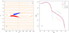 |
Fig. 16. Panel a: positions of transit (blue dots) and bounced (purple dots) particles (with EeV > 103 eV) at early acceleration stage, t = 10−5 s. Panel b: energy spectra of transit and bounced particles show that they have different spectral index: p = 0.9 and p = 1.2, respectively. The parameters for the simulated magnetic islands are identical to those in Fig. 12. The other parameters are: Ey0 = 100 V m−1, ϵ = 0.3, k = 0.003125, d = 2 m. |
4. Discussion and conclusions
In the current paper we investigate primary acceleration of particles by a steady super-Dreicer (reconnection) electric field (Dreicer 1959) induced during a magnetic reconnection process. We consider particle motion in steady 3D magnetic field topologies with a constant guiding field, which have single and multiple X- and O-nullpoints (or magnetic islands). For clarity and simplicity, the magnetic and electric fields in current sheets with a single X-nullpoint and with multiple O-nullpoints, or islands, are defined analytically. Particle trajectories and energy distributions were followed with a test particle approach for one million particles of a neutral plasma dragged in from the solar corona.
We try to establish how the particle trajectories and energy spectra are affected by the presence of multiple X- and O-nullpoints and benchmark our simulation to the results obtained in current sheets with a single X-nullpoint. This helps us to build a better understanding of the initial particle acceleration scenarios occurring in RCS with magnetic islands of different shapes and dynamics. We consider the two different magnetic topologies: first we consider coalescent or semi-similar islands with two islands moving towards each other, and second we investigate squashed islands with horizontal dimensions larger than the vertical ones. Since an acceleration time of 10−5 s for electrons is much shorter than the characteristic time (tens of minutes) of a magnetic reconnection process, magnetic field topologies are considered to be stationary allowing us to use a test-particle approach. In both the RCS topologies, that is, with either coalescent or squashed islands, we consider a reconnection electric field Ey induced by plasma inflows into the RCS diffusion region, which strongly accelerates particles from these inflows. The simulation results obtained for magnetic islands were benchmarked with those obtained in the similar 2.5D RCS with a single X-nullpoint with a constant guiding field.
It was established that in 3D current sheets with a single X-nullpoint and strong guiding field By0, particles of opposite charges have a “preferential ejection”, that is, electrons and protons become separated into the opposite semiplanes from the RCS midplane (Zharkova & Gordovskyy 2004; Pritchett 2008; Siversky & Zharkova 2009). Particles of the same charge were allowed to enter from any side of a current sheet: the side from which they enter, divides the identically charged populations into transit particles (those entering the opposite side to their subsequent ejection) and bounced particles (those entering the same side from which they are subsequently ejected) (Siversky & Zharkova 2009). We derived single X-nullpoint topologies in which particles can be unmagnetized or magnetized so that their trajectories, and ultimately their energy spectra, become essentially different. If in a current sheet the guiding field is strong, particles gain larger amount of energy for transit particles than for bounced ones (Siversky & Zharkova 2009). A new interesting effect is detected: a gyromotion about the guiding field By0 drives transit particles towards the X-nullpoint, which creates a non-transit region near the X-nullpoint. The travelling time of this gyromotion is about the time for a particle to drift from the boundary to the RCS midplane.
In a current sheet with multiple X- and O-nullpoints, or magnetic islands of any type, particles are shown to be accelerated more efficiently than in a current sheet with a single X-nullpoint. By comparing the paths of particles ejected from a magnetic island with those from a single X-nullpoint, we found that for any type of magnetic island, if there is a strong guiding field By, the concept of “preferential ejection” remains valid, similar to the acceleration in a single X-nullpoint (Zharkova & Gordovskyy 2004; Pritchett & Coroniti 2004). For example, in multiple X- and O-nullpoints there is still asymmetry of ejection for electrons and protons into different semiplanes from the midplane, similar to the asymmetry found in a single X-nullpoint reported in TP and PIC simulations (Pritchett 2008; Siversky & Zharkova 2009; Le et al. 2010).
The magnetized particles gyrate in magnetic islands around the O-nullpoint following magnetic field lines while unmagnetized particles bounce between the two nearest X-nullpoints of the island along the midplane. Once a particle gains sufficient energy to escape from the first trapping magnetic island, it does not move to the other islands (unless a strong guiding field magnetizes the particles, as shown in Fig. 10). Instead, highly energetic particles are found accumulated about the X-nullpoints gaining further acceleration from the squeezing electric field of the magnetic islands (either coalescent or squashed). As a result, the high-energy particles form electron clouds circling about the X-nullpoints (Siversky & Zharkova 2009) rather than in the middle of the O-nullpoints. Therefore, there are electron clouds formed about all the X-nullpoints between the O-nullpoints, similar to the electron clouds reported with PIC simulations with a single X-nullpoint (Siversky & Zharkova 2009; Zharkova et al. 2011). These periodic electron clouds along the current sheet midplane closely resemble the bands of energetic particles observed in-situ during crossings of the heliospheric current sheet (Khabarova & Zank 2017).
In current sheets with magnetic islands the guiding field is found to still enhance the energy gains of accelerated particles in the islands. However, the acceleration paths of particles along a reconnecting sheet are equal to the length of a single magnetic island used in the current simulations (≈ 102 m for protons), which is much shorter than the path in a single X-nullpoint (≈ 104 m). Besides the obvious dependence of particle energy gains on a reconnecting electric field Ey0, magnetic field magnitude B0, and topology, which are found to be similar to those in single X-nullpoint simulations, the dimensions and shapes of the islands are also shown to have significantly influence. Energy gains are dependent on the ratio of a reconnecting electric field to transverse magnetic field, Ey/Bx, and, thus, can be linked to the specific magnetic island configuration used in the simulations.
In the current sheet with magnetic islands, similar to a single X-nullpoint case, there is still a difference in the energy gains between the transit and bounced particles; the transit particles gain more energy than the bounced ones. In a current sheet with a strong guiding field, both types of particle become strongly magnetised leading to transit particles reaching the midplane and O-nullpoint faster, where they become accelerated, while bounced particles, being unable to reach the midplane and magnetic island, turn back instead with lower energy. Therefore, more high-energy particles are expected to come from the transit particle branch and more returning particles to come from the bounced particle branch. Furthermore, the trajectories of bounced particles are found to change their directions by 180°, with respect to the direction of their initial injection into the current sheet, that is similar to the heliospheric observations of the pitch angles of electrons of solar wind moving away from the sector boundary (HCS midplane) before they can reach this midplane (Zharkova & Khabarova 2012).
Particle acceleration in the two different types of island, coalescent and squashed, is also shown to be rather different. In general, current sheets containing multiple X- and O-nullpoints can accelerate particles more efficiently than those containing a single X-nullpoint. The electric field in squashed islands, Ey, which is parallel to (and smaller than) the reconnection electric field responsible for particle acceleration, is sufficient to boost the additional energy gains up to sub-relativistic limits within a short timescale. On the other hand, the electric field in the contracting region of a coalescent island where the two close-by islands are moving towards one another is anti-parallel to the reconnecting electric field, pushing the particles away from the islands and restraining their acceleration. As a result, the energy gains in coalescent islands are much lower than in the squashed ones. However, it must be noted that despite the overall electric field between coalescent islands being produced by the relative motion of the two islands, it does not represent the existence of any anti-reconnection process such as that found by Oka et al. (2010), which could increase the particle energy gains.
Particle energy gains ΔEes from a reconnection electric field Ey at ejection from the first O-nullpoint, or first magnetic island, are evaluated as follows.
Without a guiding field the particles gain energy ΔEes in proportion to
 for the coalescent magnetic islands, and
  for the squashed islands.
With guiding field the energy gains ΔEes are proportional to Ey for any type of islands.
The energy of ejected particles has a weak relation to the guiding field magnitude,
 .
.Particle energy gains in magnetic islands are affected by the ratios of vertical and horizontal dimensions of O-nullpoints and the ratio Ey/Bx near the X-nullpoints, following Eqs. (16) and (18).
In summary, we conclude that electrons and protons are found to be accelerated to sub-relativistic energies much more efficiently in RCS with multiple X- and O-nullpoints (magnetic islands) than in those with a single X-nullpoint. In general, we can deduce that the ranges of electron energy gains and spectral indices in magnetic islands of different shapes and dynamics in the coronal conditions discussed in the paragraphs above show a reasonably close fit to the parameters of HXR spectra observed in solar flares with the RHESSI payload (Holman et al. 2011). Particles are often found trapped inside O-nullpoints for a long time effectively gaining energy when passing through the neighbouring X-nullpoints. Some electrons form the clouds around X-nullpoints and can only escape the current sheet in the vicinity of these X-nullpoints. Obviously, the simulations carried with the test particle approach do not produce a complete picture of particle motions inside a current sheet with multiple O-nullpoints, because the plasma feedback due to the presence of accelerated particles has not yet been considered.
Further investigation is needed to uncover the effects of the plasma feedback deriving the additional electric and magnetic fields induced by the presence of accelerated particles, for example, polarisation electric field caused by separation of accelerated protons and electrons due to their asymmetric ejection towards the midplane (Siversky & Zharkova 2009) and magnetic fields induced by these particles. It would also be beneficial to consider the joint energy distributions of transit and bounced particles and the effects they can have on the ambient plasma inside a current sheet. These points will be addressed in more detail with PIC simulations discussed in a forthcoming paper.
Acknowledgments
The authors acknowledge the funding for this research provided by the U.S. Air Force grant PRJ02156. The authors deeply appreciate the constructive and useful comments provided by the anonymous referee, from which the paper significantly benefited.
References
- Bárta, M., Büchner, J., Karlicky, M., & Skala, J. 2011, ApJ, 737, 24 [NASA ADS] [CrossRef] [Google Scholar]
- Browning, P. K., & Dalla, S. 2007, Mem. Soc. Astron. It., 78, 255 [NASA ADS] [Google Scholar]
- Boris, J. P. 1970, Proceeding of Fourth Conference on Numerical Simulations of Plasmas (Washington, D. C.: Naval Research Laboratory) [Google Scholar]
- Chen, L.-J., Bhattacharjee, A., Puhl-Quinn, P. A., et al. 2008, Nat. Phys., 4, 19 [CrossRef] [Google Scholar]
- Dahlin, J. T., Drake, J. F., & Swisdak, M. 2015, Phys. Plasmas, 22, 100704 [Google Scholar]
- Dalla, S., & Browning, P. K. 2005, A&A, 436, 1103 [NASA ADS] [CrossRef] [EDP Sciences] [Google Scholar]
- Dalla, S., & Browning, P. K. 2006, ApJ, 640, L99 [NASA ADS] [CrossRef] [Google Scholar]
- Dalla, S., & Browning, P. K. 2008, A&A, 491, 289 [NASA ADS] [CrossRef] [EDP Sciences] [Google Scholar]
- Daughton, W., Roytershteyn, V., Karimabadi, H., et al. 2011, Nat. Phys., 7, 539 [NASA ADS] [CrossRef] [Google Scholar]
- Drake, J. F., Swisdak, M., Che, H., & Shay, M. A. 2006a, Nature, 443, 553 [NASA ADS] [CrossRef] [PubMed] [Google Scholar]
- Drake, J. F., Swisdak, M., Schoeffler, K. M., Rogers, B. N., & Kobayashi, S. 2006b, Geophys. Res. Lett., 33, L13105 [NASA ADS] [CrossRef] [Google Scholar]
- Drake, J. F., Opher, M., Swisdak, M., & Chamoun, J. N. 2010, ApJ, 709, 963 [NASA ADS] [CrossRef] [Google Scholar]
- Dreicer, H. 1959, Phys. Rev., 115, 238 [Google Scholar]
- Egedal, J., Daughton, W., & Le, A. 2012, Nat. Phys., 8, 321 [NASA ADS] [CrossRef] [Google Scholar]
- Fadeev, V. M., Kvabtskhava, I. F., & Komarov, N. N. 1965, Nucl. Fusion, 5, 202 [CrossRef] [Google Scholar]
- Gordovskyy, M., Browning, P. K., Kontar, E. P., & Bian, N. H. 2013, Sol. Phys., 284, 489 [NASA ADS] [CrossRef] [Google Scholar]
- Gosling, J. T., Eriksson, S., & Schwenn, R. 2006a, J. Geophys. Res. (Space Phys.), 111, A10102 [Google Scholar]
- Gosling, J. T., McComas, D. J., Skoug, R. M., & Smith, C. W. 2006b, Geophys. Res. Lett., 33, L17102 [Google Scholar]
- Guo, F., Li, H., Daughton, W., & Liu, Y.-H. 2014, Phys. Rev. Lett., 113, 155005 [NASA ADS] [CrossRef] [Google Scholar]
- Harris, E. G. 1962, Il Nuovo Cimento (1955-1965), 23, 115 [NASA ADS] [CrossRef] [Google Scholar]
- Holman, G. D., Aschwanden, M. J., Aurass, H., et al. 2011, Space Sci. Rev., 159, 107 [NASA ADS] [CrossRef] [Google Scholar]
- Hurford, G. J., Schwartz, R. A., Krucker, S., et al. 2003, ApJ, 595, L77 [Google Scholar]
- Hurford, G. J., Krucker, S., Lin, R. P., et al. 2006, ApJ, 644, L93 [NASA ADS] [CrossRef] [Google Scholar]
- Kahler, S., & Lin, R. P. 1994, Geophys. Res. Lett., 21, 1575 [NASA ADS] [CrossRef] [Google Scholar]
- Kahler, S. W., & Lin, R. P. 1995, Sol. Phys., 161, 183 [NASA ADS] [CrossRef] [Google Scholar]
- Karimabadi, H., Dorelli, J., Roytershteyn, V., Daughton, W., & Chacón, L. 2011, Phys. Rev. Lett., 107, 025002 [NASA ADS] [CrossRef] [Google Scholar]
- Khabarova, O., Zank, G. P., Li, G., et al. 2015, ApJ, 808, 181 [NASA ADS] [CrossRef] [Google Scholar]
- Khabarova, O. V., & Zank, G. P. 2017, ApJ, 843, 4 [NASA ADS] [CrossRef] [Google Scholar]
- Kliem, B. 1994, ApJS, 90, 719 [NASA ADS] [CrossRef] [Google Scholar]
- Kurth, W. S., Gurnett, D. A., Scarf, F. L., & Poynter, R. L. 1984, Nature, 312, 27 [NASA ADS] [CrossRef] [Google Scholar]
- Le, A., Egedal, J., Daughton, W., et al. 2010, Geophys. Res. Lett., 37, L03106 [NASA ADS] [CrossRef] [Google Scholar]
- Li, Y., & Lin, J. 2012, Sol. Phys., 279, 91 [NASA ADS] [CrossRef] [Google Scholar]
- Lin, R. P., Krucker, S., Hurford, G. J., et al. 2003, ApJ, 595, L69 [NASA ADS] [CrossRef] [Google Scholar]
- Lin, J., Ko, Y.-K., Sui, L., et al. 2005, ApJ, 622, 1251 [NASA ADS] [CrossRef] [Google Scholar]
- Litvinenko, Y. E. 1996, ApJ, 462, 997 [NASA ADS] [CrossRef] [Google Scholar]
- Litvinenko, Y. E., & Somov, B. V. 1993, Sol. Phys., 146, 127 [NASA ADS] [CrossRef] [Google Scholar]
- Liu, R., Lee, J., Wang, T., et al. 2010, ApJ, 723, L28 [NASA ADS] [CrossRef] [Google Scholar]
- Loureiro, N. F., Cowley, S. C., Dorland, W. D., Haines, M. G., & Schekochihin, A. A. 2005, Phys. Rev. Lett., 95, 235003 [NASA ADS] [CrossRef] [PubMed] [Google Scholar]
- Martens, P. C. H., & Young, A. 1990, ApJS, 73, 333 [NASA ADS] [CrossRef] [Google Scholar]
- Martin, Jr., R. F., & Speiser, T. W. 1988, J. Geophys. Res., 93, 11521 [NASA ADS] [CrossRef] [Google Scholar]
- Martin, Jr., R. F., Speiser, T. W., & Klamczynski, K. 1994, J. Geophys. Res., 99, 23623 [NASA ADS] [CrossRef] [Google Scholar]
- Nishizuka, N., Karlický, M., Janvier, M., & Bárta, M. 2015, ApJ, 799, 126 [NASA ADS] [CrossRef] [Google Scholar]
- Oka, M., Phan, T.-D., Krucker, S., Fujimoto, M., & Shinohara, I. 2010, ApJ, 714, 915 [NASA ADS] [CrossRef] [Google Scholar]
- Onofri, M., Isliker, H., & Vlahos, L. 2006, Phys. Rev. Lett., 96, 151102 [NASA ADS] [CrossRef] [PubMed] [Google Scholar]
- Oieroset, M., Lin, R. P., Phan, T. D., Larson, D. E., & Bale, S. D. 2002, Phys. Rev. Lett., 89, 195001 [NASA ADS] [CrossRef] [Google Scholar]
- Phan, T. D., Gosling, J. T., & Davis, M. S. 2009, Geophys. Res. Lett., 36, L09108 [NASA ADS] [CrossRef] [Google Scholar]
- Priest, E. R. 1984, Solar Magneto-Hydrodynamics (Cambridge: Cambridge University Press) [Google Scholar]
- Priest, E. R., & Forbes, 2000, Magnetic Reconnection: MHD Theory and Applications (New York: Cambridge University Press) [CrossRef] [Google Scholar]
- Priest, E., & Forbes, T. 2002, A&ARv, 10, 313 [NASA ADS] [CrossRef] [Google Scholar]
- Pritchett, P. L. 2006, J. Geophys. Res. (Space Physics), 111, A10212 [NASA ADS] [CrossRef] [Google Scholar]
- Pritchett, P. L. 2008, Phys. Plasmas, 15, 102105 [NASA ADS] [CrossRef] [Google Scholar]
- Pritchett, P. L., & Coroniti, R. V. 2004, J. Geophys. Res. (Space Physics), 109, A01220 [Google Scholar]
- Pulkkinen, T. I., Baker, D. N., Owen, C. J., Gosling, J. T., & Murphy, N. 1993, Geophys. Res. Lett., 20, 2427 [NASA ADS] [CrossRef] [Google Scholar]
- Siversky, T. V., & Zharkova, V. V. 2009, J. Plasma Phys., 75, 619 [NASA ADS] [CrossRef] [Google Scholar]
- Somov, B. V. 2000, Cosmic Plasma Physics, Astrophysics and Space Science Library (Boston: Kluwer Academic Publishers), 251 [Google Scholar]
- Song, H. Q., Chen, Y., Li, G., Kong, X. L., & Feng, S. W. 2012, Phys. Rev. X, 2, 021015 [Google Scholar]
- Speiser, T. W. 1965, J. Geophys. Res., 70, 4219 [NASA ADS] [CrossRef] [Google Scholar]
- Stanier, A., Daughton, W., Simakov, A. N., et al. 2017, J. Phys. Plasmas, 24, 022124 [NASA ADS] [CrossRef] [Google Scholar]
- Su, Y., Lee, J., Veronig, A. M., et al. 2013, Nat. Phys., 9, 2675 [Google Scholar]
- Syrovatskiǐ, S. I. 1971, Sov. J. Exp. Theor. Phys., 33, 933 [NASA ADS] [Google Scholar]
- Takasao, S., Asai, A., Isobe, H., & Shibata, K. 2012, ApJ, 745, L6 [NASA ADS] [CrossRef] [Google Scholar]
- Vilmer, N., MacKinnon, A. L., & Hurford, G. J. 2011, Space Sci. Rev., 159, 167 [NASA ADS] [CrossRef] [Google Scholar]
- Wang, R., Lu, Q., Nakamura, R., et al. 2016, Nat. Phys., 12, 263 [CrossRef] [Google Scholar]
- Wood, P., & Neukirch, T. 2005, Sol. Phys., 226, 73 [NASA ADS] [CrossRef] [Google Scholar]
- Zelenyj, L. M., Lominadze, J. G., & Taktakishvili, A. L. 1990, J. Geophys. Res., 95, 3893 [NASA ADS] [CrossRef] [Google Scholar]
- Zharkova, V. V., & Agapitov, O. V. 2009, J. Plasma Phys., 75, 159 [NASA ADS] [CrossRef] [Google Scholar]
- Zharkova, V. V., & Gordovskyy, M. 2004, ApJ, 604, 884 [NASA ADS] [CrossRef] [Google Scholar]
- Zharkova, V. V., & Gordovskyy, M. 2005a, MNRAS, 356, 1107 [NASA ADS] [CrossRef] [Google Scholar]
- Zharkova, V. V., & Gordovskyy, M. 2005b, Space Sci. Rev., 121, 165 [NASA ADS] [CrossRef] [Google Scholar]
- Zharkova, V. V., & Khabarova, O. V. 2012, ApJ, 752, 35 [NASA ADS] [CrossRef] [Google Scholar]
- Zharkova, V., & Khabarova, O. 2015, Ann. Geophys., 33, 457 [Google Scholar]
- Zharkova, V. V., Arzner, K., Benz, A. O., et al. 2011, Space Sci. Rev., 159, 357 [NASA ADS] [CrossRef] [Google Scholar]
- Zhong, J. Y., Lin, J., Li, Y. T., et al. 2016, ApJS, 225, 30 [NASA ADS] [CrossRef] [Google Scholar]
- Zhu, Z., & Parks, G. 1993, J. Geophys. Res., 98, 7603 [NASA ADS] [CrossRef] [Google Scholar]
- Zong, Q.-G., Fritz, T. A., Pu, Z. Y., et al. 2004, Geophys. Res. Lett., 31, L18803 [NASA ADS] [CrossRef] [Google Scholar]
All Tables
Comparison of different times and magnitudes of Δz for RCSs with different thickness.
All Figures
|
Fig. 1. A magnetic field topology in the vicinity of a single X-nullpoint of RCS with a thickness of 2d along the X-axis (+d and −d from X = 0) and a half width of a along the Z-axis. The particle inflows dragged in at the upper boundary (“x+”) are marked by the blue arrows and the ones at the lower boundary (“x−”) by the red arrows. The x = 0 line represents the current sheet midplane. The green lines show magnetic field lines of Bx and Bz, with the guiding field By and reconnecting electric field Ey being perpendicular to the plane of drawing. |
| In the text | |
|
Fig. 2. Left panels: simulated particle trajectories on the x−z plane. Right panels: corresponding energy gains vs. the x-coordinate of the particles. Panels a and b: sampled electrons in a simulation with d = 1 m, ξy = 0.1, B0 = 100 G, Ey = 100 V m−1. Light and dark blue lines represent the transit and bounced electrons, respectively. Panels c and d: sampled protons from the same parameters as in panels a and b, respectively. Panels d and f: trajectories of protons from a different simulation with a different d = 5 m. Panels g and h: trajectories of protons in a stronger guiding field, ξy = 1.0 and d = 1 m. |
| In the text | |
|
Fig. 3. Trajectories of selected electrons “E1” and “E2”, and protons “P1” and “P2” in Fig. 2 are plotted for the same RCS parameters as in Fig. 2 (with a guiding field By = ξB0 and ξ = 0.1); panel a: trajectories on the Z−X plane with magnetic field lines plotted in magenta as the background; panel b: energy gains by the particles vs. the x-coordinate at ejection. All the particles start from x = ± 1 m, z = 300 m. |
| In the text | |
|
Fig. 4. Panel a: energies of ejected protons vs. different Bx for fixed By0 ≡ 10−4T. Panel b: energies of ejected protons vs. different By with Bx0 ≡ 10−3 T. The energy gains from Eqs. (6) and (7) are plotted in blue and orange solid lines. The other parameters are Bz0 = 10 −3T, Ey = 250 V m−1, d = 1 m. |
| In the text | |
|
Fig. 5. Energy gains (in keV) by electrons and protons at the end of simulation vs. their initial positions ξx (t = 0). The blue triangles represent the particles starting at x = −1 m and the red dots are the ones beginning at x = 1 m. For electrons: panel a: initial velocity vx(t = 0) = 104 m s−1, panel b: vx(t = 0) = 4 × 10⁶ m s−1. For protons: panel c: vx(t = 0) = 104 m s−1, panel d: vx(t = 0) = 105 m s−1. Also, there are protons in the transit group coming back to the lower boundary, and protons in the bounced group that cross the RCS in the ξx > 0.2 region; these are marked by the green stars and purple plus symbols, respectively. The estimated maximum energy gains from Eqs. (6) and (7) are again plotted in solid blue and orange lines. The injecting ξx- coordinates of the selected electrons and protons in Fig. 2 are also marked in panels a and c. The electromagnetic fields are described in Sect. 2.1.1: B0 = 0.01T, E = 100 Vm s−1, ξy = 0.1, d = 1 m. |
| In the text | |
|
Fig. 6. Final energy gains (in keV) of the protons plotted vs. ξx at their initial positions (see Sect. 2.1.1 for more details). Panel a: for RCS with d = 40 m. Panel b: For RCS with different thickness: d = 1 m, 10 m, 40 m, 80 m, 100 m. The “x+, x+”/“x+, x−” and “x−, x+”/“x−, x−” are using the same markers to keep the picture visually clear. Equations (6) and (7) for different d are not plotted in panel b for the same reason. The other parameters are the same as described in Sect. 2.1.1: B0 = 0.01T, E = 100 V m−1, ξy = 0.1. |
| In the text | |
|
Fig. 7. Panel a: plasma inflow (green arrows) and outflow (black arrows) directions in a magnetic islands chain. The solid orange lines show the magnetic field in the x−z plane. Here islands “1” and “2” represent the squashed islands, while islands “3” and “4” represent the coalescent islands. Panel b: red dash-dot line shows the Ey from squashed islands on the midplane from Eq. (17). The blue dash line shows the Ey from coalescent islands on the midplane from Eq. (18). Here k = 0.03125. |
| In the text | |
|
Fig. 8. Test-particle orbits (left col.) and energy gains (right col.) vs. z-coordinate (blue lines), obtained during the same running simulation time, Δt = 8×10⁻⁵ s for: panel a: magnetized electron in the magnetic island described by Eqs. (14) and (16) with B0 = 100 G and the guiding field By = 0; panel b: unmagnetized electron in the magnetic island with the same dimension as panel a and B0 = 10 G; panel c: magnetized electron in the magnetic island which has the same Bx and Bz components as panel a with added guiding field By = Bz0 ξ, where ξy = 0.1; panel d: magnetized electron in the magnetic island which has the same Bx and Bz components as panels a and c but with a stronger guiding field, ξy = 1.0; and panel e: electron in the magnetic island which has the same magnetic field topology as panel a for the electric field following Eq. (17) representing squashed islands. The magnetic field lines of Bx, Bz are plotted in orange lines for all cases. Here k = 0.03125, ϵ = 0.3. |
| In the text | |
|
Fig. 9. Simulation result for a strong reconnection electric field Ey0 = 690 V m−1. Panel a: electron trajectory in the X−Z plane. The orange lines present the magnetic field in this plane. Panel b: energy gained by the electron vs. z-coordinate. The other parameters are identical to Fig. 8a: k = 0.03125, ϵ = 0.3, ξy = 0, B0 = 100 G. |
| In the text | |
|
Fig. 10. Trajectories of an electron (panel a) and a proton (panel b) accelerated in similar magnetic islands. Panel c: Trajectory of an electron in the edge island as described by Eq. (20), which has an open field topology edge at |z| > 10. d = 2 m, ϵ = 0.3, k0 = 1.0, ξy = 1. The sampled particles are all initialized at x = 0, z = 0 to reduce the computing time for the particle motion from the RCS boundaries. The orange lines present the magnetic field in the X−Z plane. Panel d: example of preferential ejection of electrons and protons from an RCS with multiple X-nullpoints. |
| In the text | |
|
Fig. 11. Left panel: different trajectories of electrons in coalescent islands for particles, which are moving away (brown and red colours) because of the contracting electric field Ey; for a “transit” electron (magenta line) moving slowly towards the midplane x = 0 for ξy = 1; for a “bounced” particle (the purple line), which takes a longer time to move into the island than for the “transit” one. The red dots represent the original positions. The magnetic field lines in x−z plane are plotted in orange. In z > 0 region, the contracting Ey < 0 area is indicated between the second and third (aqua coloured) dash lines. Right panel: energy gains versus z-coordinate of the selected “transit” and “bounced” electrons, entering the RCS at x0 = ± 2 m, z0 = 28 m. |
| In the text | |
|
Fig. 12. Panel a: different trajectories of a pair of selected transit (blue line) and bounced (purple line) electrons in a coalescent island. They enter the RCS at x0 = ± 2 m, z0 = 300 m. The magnetic field lines in the x−z plane are plotted in orange. Panel b: corresponding energy gains vs. z-coordinate of the two particles in panel a. The parameters for the simulated magnetic islands are k = 0.003125, ϵ = 0.1, B0 = 10G, ξy = 0.1. |
| In the text | |
|
Fig. 13. Panel a: energy gains by the escaping electrons (measured when they leave the first trapped island) vs. the guiding field magnitude: ξy = 0.0, 10−4, 10−2, 0.1, 0.6, 1.0. The other parameters are: Ey0 = 100 V m−1, Bz0 = 100G, ϵ = 0.3, d = 2 m, k = 0.03125. Panel b: energy gains by the escaping electrons vs. the half length of the islands: Li = 2 m, 6.4 m, 20 m, 64 m. Panel c: fluctuation of Bx on the x = 0 m plane for different aspect ratios Li/d (k−1). Panel d: corresponding fluctuation of Ey on the x = 0 plane. The other parameters are: Ey0 = 100 V m−1, Bz0 = 100G, ξy = 1.0, ϵ = 0.3, d = 2 m. |
| In the text | |
|
Fig. 14. Panel a: energy gains vs. reconnection electric field Ey for electrons at ejection from the first X-nullpoint. Panel b: energy gains vs. reconnection electric field Ey for particles ejected from the first trapping coalescence (C) and squashed (S) islands. |
| In the text | |
|
Fig. 15. Energy spectra of electrons accelerated during t = 8 × 10⁻⁵ s in the coalescent islands with magnetic field magnitudes: panel a: B0 = 100 G, and panel b: B0 = 10 G: Both ξy = 0 (the blue dash-dotted line) and ξy = 1 (red lines) cases are compared in the same plot. Panel c: energy spectrum of electrons in squashed (“S”) islands (blue dash-dotted line) with ξy = 0. For comparison, the spectrum of the ξy = 0 case in panel a from coalescent islands (“C”) is also plotted as a background. The green dotted lines indicate the initial thermal distribution with T0 = 100 eV. The other parameters are as follows: Ey0 = 100 V m−1, ϵ = 0.3, k = 0.03125, d = 2 m. We note that the dashed lines show only the referral power-law indexes in different cases and do not represent the whole fitting range of energies gained (up to three orders of magnitude on the plot). |
| In the text | |
|
Fig. 16. Panel a: positions of transit (blue dots) and bounced (purple dots) particles (with EeV > 103 eV) at early acceleration stage, t = 10−5 s. Panel b: energy spectra of transit and bounced particles show that they have different spectral index: p = 0.9 and p = 1.2, respectively. The parameters for the simulated magnetic islands are identical to those in Fig. 12. The other parameters are: Ey0 = 100 V m−1, ϵ = 0.3, k = 0.003125, d = 2 m. |
| In the text | |
Current usage metrics show cumulative count of Article Views (full-text article views including HTML views, PDF and ePub downloads, according to the available data) and Abstracts Views on Vision4Press platform.
Data correspond to usage on the plateform after 2015. The current usage metrics is available 48-96 hours after online publication and is updated daily on week days.
Initial download of the metrics may take a while.