| Issue |
A&A
Volume 620, December 2018
|
|
|---|---|---|
| Article Number | A71 | |
| Number of page(s) | 15 | |
| Section | Galactic structure, stellar clusters and populations | |
| DOI | https://doi.org/10.1051/0004-6361/201833228 | |
| Published online | 30 November 2018 | |
Local disc model in view of Gaia DR1 and RAVE data
1
Astronomisches Rechen-Institut, Zentrum für Astronomie der Universität Heidelberg, Mönchhofstr. 12-14, 69120
Heidelberg, Germany
e-mail: This email address is being protected from spambots. You need JavaScript enabled to view it.
2
Observatoire de Paris, GEPI, 77 Av. Denfert-Rocherau, 75014
Paris, France
3
E.A. Milne Centre for Astrophysics, University of Hull, Hull, HU6 7RX
UK
4
Mullard Space Science Laboratory, University College London, Holmbury St Mary, Dorking, RH5 6NT
UK
5
Department of Physics and Astronomy, Macquarie University, Sydney, NSW, 2109
Australia
6
Western Sydney University, Locked bag 1797, Penrith South DC, NSW, 2751
Australia
7
Senior CIfAR Fellow, University of Victoria, Victoria, BC, V8P 5C2
Canada
8
Université Côte d’Azur, Observatoire de la Côte d’Azur, CNRS, Laboratoire Lagrange, France
9
Observatoire astronomique de Strasbourg, Université de Strasbourg, CNRS, 11 rue de l’Université, 67000
Strasbourg, France
10
Leibniz Institut für Astrophysik Potsdam, An der Sternwarte 16, 14482
Potsdam, Germany
Received:
13
April
2018
Accepted:
27
September
2018
Abstract
Aims. We test the performance of the semi-analytic self-consistent Just-Jahreiß disc model (JJ model) with the astrometric data from the Tycho-Gaia Astrometric Solution (TGAS) sub-catalogue of the first Gaia data release (Gaia DR1), as well as the radial velocities from the fifth data release of the Radial Velocity Experiment survey (RAVE DR5).
Methods. We used a sample of 19 746 thin-disc stars from the TGAS×RAVE cross-match selected in a local solar cylinder of 300 pc radius and 1 kpc height below the Galactic plane. Based on the JJ model, we simulated this sample via the forward modelling technique. First, we converted the predicted vertical density laws of the thin-disc populations into a mock sample. For this we used the Modules and Experiments in Stellar Astrophysics (MESA) Isochrones and Stellar Tracks (MIST), a star formation rate (SFR) that decreased after a peak at 10 Gyr ago, and a three-slope broken power-law initial mass function (IMF). Then the obtained mock populations were reddened with a 3D dust map and were subjected to the selection criteria corresponding to the RAVE and TGAS observational limitations as well as to additional cuts applied to the data sample. We calculated the quantities of interest separately at different heights above the Galactic plane, taking the distance error effects in horizontal and vertical directions into account separately.
Results. The simulated vertical number density profile agrees well with the data. An underestimation of the stellar numbers begins at ∼800 pc from the Galactic plane, which is expected as the possible influence of populations from |z| > 1 kpc is ignored during the modelling. The lower main sequence (LMS) is found to be thinner and under-populated by 3.6% relative to the observations. The corresponding deficits for the upper main sequence (UMS) and red giant branch (RGB) are 6% and 34.7%, respectively. However, the intrinsic uncertainty related to the choice of stellar isochrones is ∼10% in the total stellar number. The vertical velocity distribution function f(|W|) simulated for the whole cylinder agrees to within 1σ with the data. This marginal agreement arises because the dynamically cold populations at heights < 200 pc from the Galactic plane are underestimated. We also find that the model gives a fully realistic representation of the vertical gradient in stellar populations when studying the Hess diagrams for different horizontal slices. We also checked and confirm the consistency of our results with the newly available second Gaia data release (DR2).
Conclusions. Based on these results and considering the uncertainties in the data selection as well as the sensitivity of the simulations to the sample selection function, we conclude that the fiducial JJ model confidently reproduces the vertical trends in the thin-disc stellar population properties. Thus, it can serve as a starting point for the future extension of the JJ model to other Galactocentric distances.
Key words: Galaxy: disk / Galaxy: kinematics and dynamics / solar neighborhood / Galaxy: evolution
Fellow of the International Max Planck Research School for Astronomy and Cosmic Physics at the University of Heidelberg (IMPRS-HD).
© ESO 2018
1. Introduction
In the past two decades, the amount of data collected on the Milky Way’s stellar content has increased by several orders of magnitude. A typical present-day large-scale survey contains measurements for millions of objects, and with the European astrometric mission Gaia (Gaia Collaboration 2016a, b), this number has already increased by a factor of ten. The core of the best dataset available so far for the Galactic studies includes photometry from the 2 Micron All Sky Survey (2MASS; Skrutskie et al. 2006) and Gaia G-band (Jordi et al. 2010; Carrasco et al. 2016; van Leeuwen et al. 2017), proper motions of the PPM-Extended catalogue (PPMX; Röser et al. 2008) and the fifth US Naval Observatory CCD Astrograph Catalog (UCAC5; Zacharias et al. 2017), as well as astrometric parameters of the Tycho-Gaia Astrometric Solution (TGAS; Michalik et al. 2015; Lindegren et al. 2016). Extensive information on the stellar chemical abundances is now available from spectroscopic surveys such as GALactic Archaeology with HERMES (GALAH; Martell et al. 2017), the Large sky Area Multi-Object Spectroscopic Telescope (LAMOST) General Survey (Luo et al. 2015), the Sloan Digital Sky Survey III Apache Point Observatory Galactic Evolution Experiment (SDSS-III/APOGEE; Eisenstein et al. 2011), the Radial Velocity Experiment (RAVE; Steinmetz et al. 2006), and the Gaia-ESO survey (Gilmore et al. 2012). Thus, we are entering an era in which observational data available for Galactic stellar populations will be not only various and abundant, but also precise enough to enable the detailed study of the Galactic components and to unravel their evolution. To achieve these goals, developed and robust methods are required for a comprehensive analysis of observational data.
The most sophisticated current machinery for modelling the Galaxy is the Besançon Galaxy model (BGM; Robin et al. 2003, 2012, 2017; Czekaj et al. 2014), which accounts for the stellar, gaseous, and non-baryonic content of the Galaxy. It includes the non-axisymmetry of the disc in the form of the bar and the spiral arms and the disc warp. Its first version, presented in Robin et al. (2003), is implemented in the tool Galaxia1 (Sharma et al. 2011), which allows constructing synthetic catalogues of the Milky Way and accounting for the selection effects of the different surveys. Another example of a semi-analytic model is the TRIdimensional modeL of thE GALaxy (TRILEGAL; Girardi et al. 2005; Girardi 2016), which has been designed specifically for star count simulations.
Each Galactic model has its own focus. In previous papers we developed and presented the semi-analytic Just-Jahreiß model (JJ model). Its main purpose is to enable a detailed study of the thin-disc vertical structure (Just & Jahreiß 2010, hereafter Paper I). The JJ model describes an axisymmetric thin disc in a steady state consisting of a set of isothermal stellar populations moving in the total gravitational potential. Thick and gaseous discs as well as a dark matter (DM) component are added to the general local mass budget in order to treat the pair of density-potential fully self-consistently. The main input functions describing the thin-disc evolution are the star formation rate (SFR) and age-velocity dispersion relation (AVR), as well as the age-metallicity relation (AMR) and the initial mass function (IMF). In Paper I the parameters of the JJ model were calibrated with the local kinematics of the main-sequence (MS) stars from the HIPPARCOS catalogue (van Leeuwen 2007). The model was later tested with the SDSS star counts towards the north Galactic pole, and the parameters of the thick disc were derived (Just et al. 2011, Paper II). The model IMF was constrained with the sample of HIPPARCOS data combined with the Catalog of Nearby Stars (Rybizki & Just 2015, Paper III). As discussed in Gao et al. (2013), the median model-to-data deviations over the Hess diagrams constructed with the SDSS apparent magnitudes and colours towards the north Galactic pole are 5.6% for the JJ model, but 26% for TRILEGAL and 20–53% for the old Besançon model (Robin et al. 2003).
In the long term, the development of the JJ model is focused on its extension to Galactocentric distances beyond solar. A special tool for testing chemical evolution scenarios of the Galaxy, the code Chempy2, has recently been developed (Rybizki et al. 2017). Constraining Chempy parameters with high-quality spectroscopic data and combining it with the radius-dependent SFR and AVR (first steps to the radial extension of these functions are presented in Just & Rybizki 2016 and Just et al. 2018) will be the road to build a global Milky Way disc model.
In this paper we test the JJ model locally with the high-quality astrometric data from the TGAS sub-catalogue of the first Gaia data release (DR1) and the radial velocities from the fifth data release of the RAVE survey (DR5; Kunder et al. 2017). As more than one billion stars with high-precision astrometry of the second data release (DR2) of Gaia have recently become available (published on 25 April, 2018; Gaia Collaboration 2018), the impact of Gaia DR2 on our results is also discussed.
In the framework of the JJ model, we construct the thin-disc stellar populations in the local solar cylinder, including the full stellar evolution. For the sample of mock stellar populations we predict parallaxes as observed in the TGAS×RAVE cross-match, although for the purposes of illustration, the results are presented as a function of a simple distance estimate calculated both in the data and model as the inverse observed parallax. We also account for the reddening with a realistic three-dimensional (3D) extinction model based on the map from Green et al. (2015) and simulate the complicated selection effects.
This paper has the following structure. In Sect. 2 we describe the TGAS×RAVE data sample and discuss our selection criteria together with the selection functions of the TGAS and RAVE catalogues. Section 3 explains the basics of the JJ model and the details of our modelling method. Section 4 presents the results of this study. In Sect. 5 we discuss the intrinsic uncertainty of the modelling associated with the choice of stellar library, and also the usefulness of the applied reddening map and the robustness of our results in view of more accurate and abundant Gaia DR2 data. Finally, we conclude in Sect. 6.
2. Data
2.1. TGAS×RAVE thin-disc sample
To study kinematics and spatial distribution of the thin-disc stellar populations, the full 6D information in the dynamic phase space has to be known for individual stars. The most recent and accurate five astrometric parameters, that is, positions, proper motions, and parallaxes, are provided in the TGAS catalogue. The astrometric solution was found by combining Gaia measurements of the first 14 months of the mission and information on positions from the Tycho-2 Catalogue (Høg et al. 2000). Typical errors for the parallaxes and proper motions are ∼0.3 mas and ∼0.3 mas yr−1, respectively. TGAS covers the whole sky and contains ∼2 million stars. However, this data sample alone cannot serve for our purposes as it lacks the radial velocities, which prevents deriving 3D stellar space velocity vectors. This motivated us to complement TGAS with the information from RAVE DR5 (Kunder et al. 2017), where not only accurate radial velocities are provided (typical errors are 1–2 km s−1), but also chemical abundances of six elements as well as photometry from other surveys such as 2MASS and The AAVSO Photometric All-Sky Survey (APASS; Henden et al. 2009; Munari et al. 2014). The total cross-match between TGAS and RAVE contains 257 288 stars3. For these stars we calculated the estimate of heliocentric distance by inverting the TGAS parallaxes,  . Here and elsewhere in this paper, notations with tilde are used to emphasise that a given quantity is related to the observed distance derived through this simple inversion. We also transformed it to the distance from the Galactic plane
  . Using the TGAS proper motions and parallaxes as well as the RAVE radial velocities, we calculated for each star a 3D velocity in Cartesian coordinates (U, V, W). The components of the peculiar velocity of the Sun were chosen as U⊙ = 11.1 km s−1, W⊙ = 7.25 km s−1 (Schönrich et al. 2010), V⊙ = 4.47 km s−1 (Sysoliatina et al. 2018). Currently, only the vertical motion of stars is included in the JJ model, such that only the W component of the spatial velocities is used in practice. We also calculated the observational errors (ΔU, Δ V, Δ W) with the help of the TGAS error covariance matrix.
The present-day version of the JJ model contains a detailed recipe for constructing the individual populations of the Galactic thin disc while the other components are added in a simple way. Thus, to perform a detailed model-to-data comparison, we needed to construct a clean thin-disc sample from the data. To do so, we applied the following selection criteria to the TGAS×RAVE cross-match.
-
Geometry cut. We selected stars with |b| > 20° as the RAVE survey avoids the Galactic plane and the number of observed stars drops quickly at low Galactic latitudes. As later we account for the incompleteness of the selected sample, we considered only a special region on the sky where the selection function of the TGAS catalogue is defined (Bovy 2017). We further selected only stars below the Galactic plane,
 , as after all the cuts listed in this section the fraction of stars left above the midplane is only 6.6% of the total final sample, which can be safely neglected in order to reduce the modelled volume and thus speed up the calculations. We also restricted ourselves to the local cylinder by applying
  pc and
  kpc. Hereafter we drop modulus in our notation of height and recall that our model is plane-symmetric and we work in the region below the midplane. The number of stars left is 51 234.
 -
Parallax cut. About 1.3% of the stars in the TGAS×RAVE cross-match have negative parallaxes because of the impact of large observational errors on astrometric solutions for faint and/or distant stars. As a straightforward conversion 1/ϖ is not applicable in this case, we further included only stars with positive parallaxes, ϖ > 0. Next we selected stars with a relative parallax error smaller than 30%, σϖ/ϖ < 0.3. After this cut, 50 491 stars remained.
-
Photometric cut. We selected stars with known (B − V) APASS colour that belonged to the range of visual magnitudes and colours prescribed by the observation windows of the RAVE and Gaia surveys: 7 < IDENIS/mag < 13, 0 < (J − Ks)2MASS/mag < 1 and 0 < J2MASS/mag < 14. The remaining sample contains 45 478 stars.
-
Quality cut. We set a lower limit to the signal-to noise ratio (S/N) of the RAVE spectra, S/N > 30. We also selected only stars with algo_conv ≠ 1, which corresponds to the robust stellar parameters derived from the RAVE spectra. Additionally, we ensured that only stars with reliable values of TGAS astrometric parameters entered our sample. For this we applied the cuts to astrometric excess noise, ϵi < 1, and its significance, D[ϵi]> 2. At this stage, 34 501 stars were left.
-
Abundance cut. To select the stars that can be identified as thin-disc members in chemical abundance plane, we first applied the cut 4000 < Teff/K < 7000 as only for this range of effective temperatures the chemical abundances were determined in RAVE (Kunder et al. 2017). Then the cuts [Fe/H] > −0.6, [Mg/Fe] < 0.2 were added. As discussed in Wojno et al. (2016), this is a reasonable criterion for the separation of the thin and thick discs in the RAVE data.
After applying all the selection criteria, we had a sample of 19 746 stars (Fig. 1, blue). The numbers of stars given for each stage of the data cleaning should not be interpreted straightforwardly in terms of strictness of the applied criteria. Because of the strong correlations between some of the criteria (e.g. cuts 1 and 2), these values are very sensitive to the order of applying the cuts. Alternatively, all the criteria might be sorted according to the origin of the quantities and the fractions of stars might be estimated that were removed from the initial sample due to the problems with TGAS or RAVE or even entries from TGAS and RAVE together. The corresponding fractions removed from the sample after a simple geometric pre-selection (300-pc radius, −1000 pc <  < 0 pc) were 38%, 14.5%, and 22%, respectively.
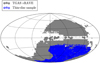 |
Fig. 1. Sky coverage of the data in the Galactic coordinates. The full TGAS×RAVE cross-match is shown in grey. The selected thin-disc sample (blue) lies below the Galactic plane; its special shape at b < −50° reflects the Gaia scanning law pattern. |
2.2. Data incompleteness
By reducing the TGAS×RAVE cross-match with criteria 1–5, we selected a clean thin-disc sample in the local solar cylinder with high quality of the measured quantities. This final sample is not representative for the direct study of the vertical disc structure, however: the TGAS and RAVE catalogues are both incomplete, and the applied cuts exacerbate this incompleteness. To account for this, we thoroughly examined the sources of possible biases in our sample and constructed its selection function for further practical use.
The final thin-disc sample clearly contains imprints of the selection functions from both of its parent catalogues. The selection function of the RAVE DR5 depends in general on I-band photometry, J − Ks colour, and position on the sky, SRAVE(α, δ, I, J − Ks). However, the dependence on colour is relevant only for the low latitudes, 5 ° < |b|< 25° (Kordopatis et al. 2013; Wojno et al. 2017) and is not of primary importance. The selection function of RAVE DR5, which was derived recently in Wojno et al. (2017) and is used in this paper, ignores the colour dependence, SRAVE(α, δ, I). The completeness factor of the RAVE data varies strongly with the line of sight and visual I-band magnitude. The TGAS selection function was investigated in Bovy (2017) and was found to be quite homogeneous over a large part of the sky. It is defined in terms of 2MASS magnitudes and colours, STGAS(α, δ, J − Ks, J). Because of the properties of the Gaia scanning law, the number of observations per star in Gaia DR1 is lowest near the ecliptic, that is, the measured quantities in the near-ecliptic regions are characterised by high uncertainties and are expected to be most biased by systematic errors. For this reason, near-ecliptic “bad” regions were excluded from the analysis in Bovy (2017), such that the TGAS selection function is not defined for the whole sky. We considered only the region where the TGAS selection function is known (cut 1).
Our selection criteria listed in Sect. 2.1 also add to the total incompleteness of the final sample. The first cut specifies the geometry of the modelled volume and is of no interest here. The parallax cut was modelled as described in Sect. 3.5. We also lost stars when applying the high-quality criteria (cut 4) together with the selection of stars with available APASS colour (part of cut 3). Finally, not all of the stars in the volume have measurements of Fe and Mg, even within the safe effective temperature range given. As a result, by applying cut 5, we also removed a part of the upper main sequence (UMS) and lost thin-disc stars. To quantify the fraction of the thin-disc stars missing in our final sample, we constructed two additional data sets. The first contains stars with known chemical abundances that are classified as thin-disc populations but have low-quality or incomplete records (if any condition from cut 4 is not fulfilled or the APASS (B − V) colour is missing). The second data set contains stars that are unclassified as a result of missing chemical abundances, regardless of the quality of their spectra and astrometric solution or available photometry. At this point, we can derive a reliable estimate of the missing star fraction. To determine the total number of thin-disc stars in some vertical bin that also pass our parallax cut, we summed all the three samples in the following manner:
 (1)
(1)
where Nf, Nσ, and Nx are the number of stars in the final, low-quality, and unclassified samples. The densities ρd and ρt are the local vertical density profiles of the thin and thick discs as inferred in Paper I and Paper II, respectively. The two limits  and
and  are the boundaries of the corresponding vertical bin. In order to simplify the expression, we dropped the dependence on
  of all quantities in this equation. With this estimate we calculated the total fraction of the missing stars Ftot as a function of height:
 (2)
(2)
Here Fσ and Fx are the fractions of stars that are missing in our final clean thin-disc sample because of the high noise and the absence of chemical abundances, respectively. The fractions given by Eq. (2) are shown in the top panel of Fig. 2. All three curves are smoothed with a window of 10 pc width. After summation over all vertical bins, we find that ∼37% of the total expected number Ntot are missing in our final sample.
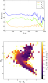 |
Fig. 2. Top: fraction of stars missing in the solar cylinder of 300 pc radius and 1 kpc height below the midplane. The orange line corresponds to the contribution from the low-quality stars, and the green curve gives an upper limit on the fraction of stars that did not enter the final sample because of the missing chemical abundances. The total fraction of missing stars is shown in blue. Bottom: total fraction of the missing stars as a function of absolute G magnitude and G − Ks colour. |
We also examined the fraction of missing stars in the Hess diagram. The bottom panel of Fig. 2 with the Ftot ratio calculated in colour-magnitude bins for the whole cylinder shows that the unclassified stars mostly influence the UMS; the LMS and red giant branch (RGB) regions are affected to a somewhat smaller extent. As it is not fully clear which of the unclassified stars really belong to the thin disc (the ratio of the thin- and thick-disc densities presented in Eq. (1) was used only to estimate the number of stars, it gives us no clue which population an individual star belongs to), we did not attempt to use the derived weights of the Hess diagram as an additional selection function during the modelling procedure. We rather kept it as a key for understanding the nature of the discrepancies between the data and model when they arose (see Sect. 5).
Now, treating all the described selection effects as independent, we defined a completeness factor for the TGAS×RAVE thin-disc sample as follows:
 (3)
(3)
Here  corresponds to the selection effect arising from the parallax cut (practical realisation described in Sect. 3.5).
  is the additional completeness factor related to the missing stars problem. All the factors of the selection function except for SQ were applied at the creating of the stellar populations and calculating of the quantities of interest such as Hess diagrams or velocity distribution functions, whereas SQ was taken into account at the post-processing of the results (Sect. 3).
3. Model and simulations
3.1. Basics of the JJ model
Our self-consistent chemodynamical model of the thin disc has been presented and discussed in a series of papers. We refer to our original Paper I for the model details and also for Paper II and Paper III for its later improvement. Here we briefly review the model basics that are relevant for the further discussions.
The thin disc is constructed from a set of 480 isothermal monoage subpopulations with ages in the range of τ = 0…12 Gyr with an equal step of Δτ = 25 Myr. The dynamical heating of the subpopulations is given by the AVR function, which describes an increase in vertical velocity dispersion with stellar age as a result of the response to small perturbations in the gravitational potential. We model the AVR as a power law with the vertical velocity dispersion starting at ∼5 km s−1 for the newly born stars and increasing up to 25 km s−1 for the oldest subpopulation. Another input function of interest is the SFR, which is implemented as a two-parametric analytic function. When combined with the AVR and IMF, it is a sensitive tool to predict star counts and age distributions. A local chemical enrichment in terms of a monotonously increasing AMR is added to the model in order to reproduce the observed metallicity distributions. In addition to the thin disc, other Galactic components are included in the total mass budget. The gas is modelled with the scaled thin-disc AVR, its scale height was optimised to hg = 100 pc in order to reproduce the observed surface density of the gas. The thick disc is included as a single-birth population with an age of 12 Gyr. The spherical isothermal DM halo is added in a simple thin-disc approximation. The thin-disc subpopulations are assumed to be in dynamic equilibrium in the total gravitational potential generated by the stellar, gaseous, and DM components of the Galaxy. By solving Poisson’s equation iteratively, we obtain a self-consistent vertical potential and density laws of the thin-disc subpopulations. Originally, the AVR parameters were calibrated against the kinematics of MS stars from the HIPPARCOS catalogue combined at the faint end with the Fourth Catalogue of Nearby Stars (CNS4; Jahreiß et al. 1997). To constrain the AMR, the local metallicity distribution from the Copenhagen F and G star sample (GCS1; Nordström et al. 2004) was used (Paper I). The thin-disc vertical profile is essentially non-exponential close to the plane, characterised by half-thickness hd = 400 pc. However, kinematic data alone do not help to distinguish SFR and IMF. Further comparison of the model to the Sloan Digital Sky Survey (SDSS) star counts towards the north Galactic pole allowed us to distinguish the SFR and IMF (Paper II) and constrain both of them (Paper II; Paper III). Our best SFR has a peak at τ ≈ 10 Gyr and is characterised by the mean and present-day star formation rate of 3.75 M⊙ pc−2 Gyr−1 and 1.4 M⊙ pc−2 Gyr−1, correspondingly. At this stage, the thick-disc parameters were also improved. The local surface density was set to 5.4 M⊙ pc−2 (18% of the thin-disc surface density), the scale height was fixed to ht = 800 pc, and the vertical velocity dispersion was σt = 45.4 km s−1.
We note that although numerous recent studies indicate that the thick disc might be more complex than we adopt here (e.g. Bovy et al. 2012a, b; Haywood et al. 2013), the topic is still under debate. It is generally recognised that the thick disc is an old, alpha-rich, and metal-poor population formed on a short timescale. The span of the suggested timescale varies significantly in different studies (4–5 Gyr in Haywood et al. 2013, but less than 2 Gyr with as low as 0.1 Gyr in the two-infall chemical models in Grisoni et al. 2017, 2018). Some authors (Haywood et al. 2013; Hayden et al. 2017) reported an increase in vertical velocity dispersion with the age of thick-disc populations. On the other hand, within the framework of the Jeans analysis developed in Sysoliatina et al. (2018), the alpha-rich metal-poor thick disc behaves as a well-mixed kinematically homogeneous population. As the local data alone are not enough to distinguish the thin and thick discs in a robust way, we did not attempt to re-define them in this work. For a quick test against Gaia DR2 (see end of Sect. 5), we modelled the thick disc with a metallicity spread. Further possible improvements are postponed to the stage when the model is fully extended, which will also include the detailed chemical evolution. This will allow us to study different Galactic populations in the abundance plane.
Thus, at the moment we arrived at a monotonous AVR and AMR, a decreasing SFR, and a three-slope broken power-law IMF for the thin disc and a single-age, scale height, and vertical velocity dispersion thick disc. Following the convention established in Paper I–Paper III, we address this best set of parameters as the fiducial model A and use it for the modelling throughout this paper.
3.2. Modelling procedure
Before going into the details, we sketch a general overview of the modelling procedure summarising all steps discussed below in Sects. 3.3–3.7.
We start with discretisation of the age-metallicity space and assigning an isochrone to each age-metallicity pair (Sect. 3.3). After this, we create a cylindrical grid (Sect. 3.4) and populate each of its space volumes with the predicted types of stars (characterised by age, metallicity, and mass from the isochrone) and take into account the parallax cut (Sect. 3.5), reddening, the TGAS×RAVE selection function (Sect. 3.6), and the corresponding abundance and photometric cuts. Then we account for the vertical effect of the distance error (Sect. 3.7) and investigate the properties of the mock sample as a function of distance from the midplane (Sect. 4).
3.3. Creation of the stellar assemblies
We started our modelling with thin-disc mono-age subpopulations. Each age corresponds to a unique value of metallicity as prescribed by the AMR law. We added a Gaussian scatter in metallicity σ[Fe/H] = 0.15 dex. Each age τi was then associated with seven metallicities representing a Gaussian with a mean AMR(τ) and a dispersion σ[Fe/H]. Each metallicity subpopulation is given an appropriate weight wk, such that  . In Paper I a similar scatter in metallicity was modelled to reproduce the observed metallicity distributions of Geneva–Copenhagen F and G stars, which can be interpreted either in terms of observational errors or in terms of real physical scatter in metallicity of mono-age populations. The added dispersion σ[Fe/H] here corresponds to a physical scatter in metallicity as the age-metallicity grid was then used to select isochrones. This complexity roughly accounts for the effect of radial migration, which is not explicitly introduced in our model.
At this point, it is useful to define a new notation in order to avoid confusion in the future. From here on, we refer with “subpopulation” to the thin-disc mono-age isothermal subpopulations. For the additional splitting in metallicity-mass parameter space, we introduce the term “stellar assembly”. Thus, the described splitting of the subpopulations in metallicity results in 480 ⋅ 7 = 3360 stellar assemblies.
The next step is to include the full stellar evolution. We used the Modules and Experiments in Stellar Astrophysics (MESA; Paxton et al. 2011, 2013, 2015) Isochrones and Stellar Tracks (MIST; Dotter 2016; Choi et al. 2016)4. We took a set of 67 isochrone tables that safely cover the whole range of the modelled metallicities, [Fe/H] = −0.6…0.46. The ages of isochrones are given in logarithmic range log(τ/yr) = 7…10.08 with a step of 0.02. Each of the 3360 stellar assemblies constructed earlier was associated with the isochrone that had the closest age and metallicity to the modelled ones. The MIST isochrones cover a range of initial masses 0.1…300 M⊙ from which we selected the range 0.1…100 M⊙ as prescribed by the model IMF. The resulting number of the stellar assemblies characterised now by the same ages, metallicities, and initial stellar masses is ∼5 × 10⁶. For each stellar assembly j, a surface number density  was calculated by weighting the SFR with the IMF and accounting for the weights wk. Isochrones also provide us with the present-day stellar masses, stellar parameters log L, log Teff, log g, and absolute magnitudes in the standard UBVRI system, 2MASS JHKs, and Gaia G band. At this step, we have a table of the mock stellar assemblies with their known surface densities in the solar neighbourhood. The remaining modelling procedure may be briefly described as checking which of these types of stars were actually observed in the TGAS×RAVE cross-match and then were selected by us for the thin-disc sample as well as for further distributing them in the local cylinder.
The volume number density is calculated by
 (4)
(4)
where  is the surface number density of a given stellar assembly, h(τj) and σW(τj) are the half-thickness and the vertical velocity dispersion defined by the AMR for the corresponding age τj, respectively, and Φ(z) is the total vertical potential at a height z, as predicted by the fiducial model A. As an example outcome of the local model, we calculated the volume densities NV at z = 0 kpc for all modelled stellar assemblies and constructed a Hertzsprung–Russel (HR) diagram for the thin disc in the solar neighbourhood (Fig. 3).
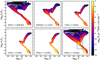 |
Fig. 3. Theoretical HR diagrams for the thin disc as predicted by the local JJ model with the use of MIST isochrones. Five age bins illustrate the contributions from the different thin-disc populations to the total HR diagram (lower right). The blue box roughly corresponds to the region studied in this work. |
Before proceeding to the next steps of the modelling, we pre-selected stellar assemblies with the effective temperatures belonging to the RAVE range (cut 5). An additional pre-selection was based on the expectations for the range of absolute G magnitudes in the sample, which we set to −2…10 mag (see bottom panel of Fig. 2). The reduced subset of the stellar assemblies used further during the simulations falls into the blue frame on the bottom right plot in Fig. 3.
3.4. Sample geometry
To model the geometry of the thin-disc sample, we created a 3D grid in cylindrical coordinates (r, θ, z). To adequately account for the parallax cut (see below), we set the initial radius of the cylinder to rin = 500 pc. This is larger than we used for the data (cut 1 in Sect. 2.1). The modelled cylinder extends vertically up to zmax = 1 kpc below the midplane. The region above the Galactic plane was not included. We binned this cylindrical volume (1) in height z with a step of Δ z = 5 pc, (2) in angle θ, which was measured from the cylinder axis, with a step of Δ θ = 3°, and (3) in radial direction r by binning the space in 20 intervals in logarithmic scale. This gives 4.8 × 10⁵ space volumes, but only those of them that correspond to the directions of observations were used in the actual modelling.
3.5. Parallax cut
The distances r and z defining the model grid are not directly comparable to the distance estimates derived for the data sample through the inversion of observed parallaxes. As a work-around, we translated the model true distances into the space of observed parallaxes. This allowed us to include in the model the same parallax cut as was applied to the data, and also to account for the distance error effects.
We split the procedure into two independent steps. First, we applied Eq. (5) at fixed z and translated the model distances to the observed parallaxes. This allowed us to reduce the number of the stellar assemblies left for the modelling at a given height by applying a parallax cut identical to the one we introduced in Sect. 2.1. Then we reduced the radius of the modelled cylinder to 300 pc using the distances calculated from the mock observed parallaxes. At this stage, we treated different z-slices as independent, that is to say, the modelled stellar assemblies remained at their initial height. The fact that a given star is observed at  different from its true distance from the midplane z was taken into account at the second stage during a post-processing of the quantities calculated in the different z-slices. This strategy was chosen in order to simplify the modelling process and speed up the calculations, as it allowed us to include the effect of the distance error in vertical direction at the post-processing stage of the simulations. We now consider the first step with the parallax cut more closely; the second step is described in Sect. 3.7.
We started with the usual assumption that the observed parallax ϖ is distributed normally about the true parallax p = 1/d with a standard deviation σϖ depending on the stellar brightness, exposure time, and number of observations per star. This is a good approximation of the real shape of the TGAS parallax error distribution, which is known to deviate slightly from normality only beyond ∼2σ (Lindegren et al. 2016). Under this assumption, the normalised probability of the observed parallax ϖ is given by the Gaussian PDF:
![Mathematical equation: $$ \begin{aligned}&P(\varpi |\sigma _{\varpi },p) = \frac{1}{A} \exp {\Big [ - \frac{(\varpi - p)^2}{2 \sigma _{\varpi }^2} \Big ]}\cdot \nonumber \\&\qquad \mathrm{with} \ A = \sqrt{2 \pi } \sigma _{\varpi }. \end{aligned} $$](/articles/aa/full_html/2018/12/aa33228-18/aa33228-18-eq20.gif) (5)
(5)
An example PDF of the observed parallax is shown in the inset of Fig. 4.
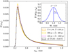 |
Fig. 4. Normalised parallax error PDF as taken from the full TGAS×RAVE cross-match (black). The orange, yellow, and violet histograms correspond to the PDFs of the subsamples with different distance ranges. The similarity of their shapes demonstrates an independence of the parallax error from the parallax itself (i.e. the distance). In the inset an example normalised Gaussian PDF for the observed parallax is plotted. The true parallax and its observational error are set to 1 and 0.3 mas, respectively. |
At each fixed height z, we have 2400 volume spaces, as implied by the model grid. We assumed that the parallax error PDF as derived from the TGAS×RAVE cross-match (Fig. 4, black histogram) does not depend on parallax or direction of observation (see coloured PDFs in Fig. 4). After this, we can easily assign parallax errors to our stellar assemblies when modelling the stellar content in each volume space. Then the observed parallaxes can be derived from the Gaussian distribution in accordance with Eq. (5). We performed this separately for each radial bin in a given z-slice. In summary, at each fixed z, we selected a pie of 20 space volumes corresponding to the same angle θ and different distances from the cylinder axis, and in each of them, we reduced the table of stellar assemblies in the following way:
-
A random true heliocentric distance d within the given space volume was assigned to each stellar assembly and was then converted into the true parallax p = 1/d.
-
Parallax errors σϖ were drawn randomly from the parallax error PDF.
-
The corresponding observed parallaxes ϖ were derived as random values from the Gaussian PDF P(ϖ|σϖ, p).
-
The observed parallaxes ϖ were converted into observed distances
 .
. -
Cuts identical to those used for the data sample were applied: ϖ > 0, σϖ/ϖ < 0.3.
-
Only stellar assemblies with
 pc were selected. This allowed us to account for the fact that the parallax errors cause some stars that lie outside the modelled cylinder to be observed within it (alternatively, stars that actually belong to the cylinder of 300 pc radius may appear at larger distance and be excluded from the sample).
 -
We also removed the stellar assemblies located at |b|< 20° to reproduce the spatial geometry of the modelled sample.
The resulting set of tables of the stellar assemblies were then subjected to the TGAS×RAVE incompleteness factor.
3.6. TGAS×RAVE selection function
After the parallax cut was applied, in each space volume at a given z we calculated the visual magnitudes in the I and J bands as well as colour (J − Ks) for all the stellar assemblies that were left. Apparent or absolute magnitudes in other photometric bands such as B, V, or G were also added when necessary. Visual magnitudes were calculated with the true model distances d.
The recent progress in mapping the dust content of the Milky Way allowed us to use a fully realistic 3D extinction model instead of the 2D map of Schlegel et al. (1998; Paper II) or the simple analytic extinction model from Vergely et al. (1998; Paper III). We implemented the 3D dust map from Bovy et al. (2016)5, which is a combination of 3D extinction models from Drimmel et al. (2003), Marshall et al. (2006), and Green et al. (2015).
The photometric cuts 7 < I/mag < 13, 0 < (J − Ks)/mag < 1 and 0 < J/mag < 14 were then applied to the stellar assemblies, in full analogy with the corresponding data selection criterion (cut 3, Sect. 2.1). The surface number densities of the remaining stellar assemblies were weighted with the completeness factor SRAVE × STGAS. For this we binned the stellar assemblies in I and J magnitudes with the corresponding steps of Δ I = 0.5 mag and Δ J = 0.1 mag as well as in colour (J − Ks) with a Δ (J − Ks)=0.14 mag step. After this, we calculated the resulting stellar number in a given grid cell by converting the surface stellar densities  into
into  in accordance with Eq. (4) and multiplying the volume density by the volume of the cell. With the known number of stars as well as their multi-band photometry, ages, and metallicities, we can predict the vertical density laws for different populations, calculate vertical kinematics with the AVR, and study the modelled sample in the colour-magnitude plane.
3.7. Vertical distance error
At the stage of post-processing the results, when the quantities of interest were calculated for different z, we also accounted for the effects of the distance errors in the vertical direction. To do so, we introduced a probability  , which defines a likelihood for a quantity Q calculated at its true z to be observed at another height
  given a corresponding vertical error σz. In order to derive the
  expression, we rewrote Eq. (5) in terms of heliocentric distance:
![Mathematical equation: $$ \begin{aligned}&P(\tilde{d}|\sigma _d,d) = \frac{1}{B} \exp {\Big [ - \frac{d^4}{\sigma _d^2} (1/\tilde{d} - 1/d)^2 \Big ]} \nonumber \\&\quad \;\;\mathrm{with} \ B = \int _{0}^{\infty } P(\tilde{d}|\sigma _d,d)\,\mathrm{d} \tilde{d}, \end{aligned} $$](/articles/aa/full_html/2018/12/aa33228-18/aa33228-18-eq28.gif) (6)
(6)
where  and d are the observed and true heliocentric distances and σd is the distance error. At this point, we need to know how both distances as well as the distance error correspond to the true and observed heights, that is, the functions of interest are
  , d(z) and σd(z). The first can be easily derived from the thin-disc sample itself (blue curve in the top panel of Fig. 5). Its behaviour is ruled by the sample geometry. Owing to the cut |b| > 20°, close to the midplane the radius of the cylinder grows linearly with
  until it reaches 300 pc, so that the mean distance
  increases almost linearly with height. At large
  the mean distance asymptotically approaches
  . The function d(z) can be calculated within the model framework, but for our accuracy, it is sufficient to use an approximation
  . Then the distance error is estimated as σd(z)=1/d2(z)⋅σϖ with a constant σϖ = 0.3 mas, which is a typical parallax error of the TGAS catalogue (magenta curve in the top panel of Fig. 5).
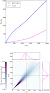 |
Fig. 5. Top: mean observed heliocentric distance |


The vertical effect of the distance error is illustrated in the bottom panel of Fig. 5. The colour-coding represents the normalised probability P( <
<  <
<  ).
).
The two projections of this diagram are of special interest. The vertical projection, calculated for a true height z = 500 pc, gives a skewed PDF that describes a likelihood for a star located at z to be observed at other heights  ,
,  . The horizontal projection shown for the same but observed height
  pc describes the impact from the different vertical bins on a given
  , which is expressed with the PDF
  . While the maximum of the probability density
  belongs to a slightly larger height than the corresponding true z, the shift is opposite in case of
  : a star observed at a given
  most probably belongs in reality to a smaller height. It is also clear that the vertical effect of the distance error is negligible close to the midplane, where the distance errors are small, and has the largest impact on the location of the most distant stars. We also have to consider heights larger than zmax = 1 kpc in order to allow the stars to not just leave the cylinder, but also to enter it from the larger heights (in full analogy with the radial direction, when we first consider a cylinder of a larger radius and then cut it to 300 pc after allowing stars to migrate horizontally due to the distance error effect). However, as the stellar density decreases approximately exponentially with increasing height, we expect the effect of not including z > zmax to be very small except in the most distant parts of the cylinder, so we did not model it.
Finally, we write
 (7)
(7)
With Eq. (7) we calculated the quantities of interest as functions of observed height  :
:
 (8)
(8)
Here an additional and final correction was included in the form of the  factor discussed in Sect. 2.2. Alternatively, when we wish to derive the model predictions in the horizontal slice of a thickness of
  , we write
 (9)
(9)
Equations (8) and 9 are used to account for the vertical effects of the distance error for the modelling of the stellar density laws and vertical kinematics. An alternative procedure for the Hess diagrams is presented in Sect. 4.3.
4. Results
4.1. Vertical density law
The first and most straightforward test that can be conducted with the JJ model is a comparison of the observed and predicted vertical density profiles because the primary focus of the model is the vertical structure of the stellar populations in the disc. By following the steps described in Sects. 3.3–3.7, we calculated the vertical stellar density law for all stars in the cylinder,  with
with  being the volume of the corresponding vertical bin. The top panel of Fig. 6 shows the stellar number density as calculated from the data (blue line) and as predicted by the model (violet and red curves). The final model prediction is plotted in red, while the violet curve is given for comparison to show the number density law as predicted without the impact of the vertical distance error taken into account. The procedure of weighting the model output with the PDF
  results in migration of stars to larger observed heights
  , which in turn leads to a better consistency with the data far from the midplane. On the other hand, the effect is very small close to the Galactic plane, predictably in view of the negligible distance error in close vicinity to the Sun (Fig. 5, top panel). The observed and the modelled density profiles agree well at all heights, which also implies a good agreement in the local region close to the Galactic plane where the model is well calibrated and is therefore expected to produce robust predictions. By analogy to the vertical profiles, we derived a distribution of stars over the observed heliocentric distances that allows us to quantify the model-to-data agreement in spherical volumes as well. The error in the predicted stellar number within a 25 pc local sphere (considered for the model calibration in Paper III) is ∼6%. However, we note that the actual number of observed stars in this volume is smaller than ten, such that the statistics is strongly influenced by Poisson noise.
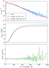 |
Fig. 6. Top: volume number density of stars in the modelled cylinder. The blue line represents the data, and violet and red curves are the model predictions before and after the vertical error effect is taken into account. Middle: cumulative number of stars in the cylinder as a function of observed height |

When investigated in terms of the cumulative number of stars as a function of observed height, the model and data demonstrate 7.8% disagreement at  kpc (Fig. 6, middle panel). The ratio of the observed to modelled stellar number in individual vertical bins as shown in the bottom panel of Fig. 6 helps to understand the systematic trends in the model-to-data differences. The ratio is close to unity over a wide range of heights, which means that the robustness of the modelled vertical profile and our treatment of the stars that are missing in the volume as a result of the lack of chemical abundances and low quality of other parameters are reliable (Fig. 2). It is also clear that starting from ∼600 pc, the Poisson noise begins to dominate star count statistics in the bins. From a height of approximately 800 pc, the number of stars is systematically under-represented in the model. Consistently, we expect this region to be biased in our simulation as we did not model stars at heights larger than 1 kpc and thus did not account for their possible presence in our sample owing to the large distance errors.
It is also interesting to perform a comparison in the space of observed parallaxes in order to validate our two-step treatment of the parallax uncertainties and the vertical distance errors. Following our standard steps, we calculated the parallax distributions at individual model heights z and then weighted the results with the corresponding probabilities  and completeness factors
  . The final distribution is shown in Fig. 7. Both data and model are normalised to the total number of observed and predicted stars, such that the shapes of the distributions can be clearly compared. We find a very good agreement between the two curves, which demonstrates the reliability of our forward-modelling approach.
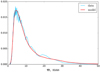 |
Fig. 7. Normalised parallax distributions as derived from the TGAS×RAVE thin-disc sample and as predicted by the JJ model. |
4.2. Vertical kinematics
It is illustrative to test the model performance in terms of the vertical kinematics that was originally used to calibrate the model parameters (Paper I). Again, following the routine described in Sects. 3.3–3.7, we evaluated for each observed height  the velocity distribution function f(|W|) as a superposition of Gaussians with the standard deviations given by the AVR. We considered the absolute W-velocities in a range of 0…60 km s−1 with a step of Δ|W|=2 km s−1. The width of the step was selected such that it allowed tracing the shape of the velocity distribution function but at the same time was larger than the typical observational error in the velocity bin. Following Eq. (9), we modelled f(|W|) in six horizontal slices probing the dynamical heating of the disc as a function of distance from the midplane. The observed and predicted normalised velocity distribution functions calculated for the different ranges in
  as well as for the whole cylinder are shown in Fig. 8. Green points represent the data with the error bars calculated as standard deviation of the Poisson distribution. The red curves are the model predictions. In general, the observed and modelled vertical kinematics of the sample agree very well. The total predicted f(|W|) (Fig. 8, right plot) is consistent with the data within 1σ at almost all |W|. This is also true for the velocity distribution functions compared to the data at different heights (Fig. 8, three left columns). A noticeable discrepancy appears in the two lowest bins, for 0 pc
  100 pc and 100 pc
  200 pc, where the fraction of the dynamically cold populations is underestimated in our model. In general, a trend with height is clearly evident: with the increase of the distance to the midplane, the shape of f(|W|) becomes less peaked at small |W|. This is a natural and straightforward result as more dynamically heated populations reach larger distances from the Galactic plane because their velocities are higher.
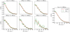 |
Fig. 8. Normalised velocity distribution functions f(|W|) for the six horizontal slices (3 × 2 plots on the left). The right graph shows f(|W|) for the whole modelled cylinder. |
We also compared f(|W|) in four magnitude bins, for which we selected different parts of the MS (CMD in Fig. 9). The bin ranges were the same as used in our previous work (compare to Fig. 3 in Paper I). The CMD shows the whole TGAS×RAVE thin-disc sample colour-coded with the RAVE metallicity. A metallicity gradient across the MS is visible such that each of the defined magnitude bins contains a mixture of stars with different metallicities and ages. To model f(|W|) for the selected magnitude bins, we added the same colour-magnitude cuts to the calculation procedure and removed the stars that did not fall under the given criteria after adding the reddening, at the stage of applying the TGAS×RAVE selection function (Sect. 3.6). The remaining calculation procedure was the same. The velocity distribution functions for the MS also show a good consistency with the data (Fig. 9, left), although the model slightly underestimates the role of the dynamically cold populations for the bin 3.5 mag < MV < 4.5 mag.
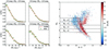 |
Fig. 9. Normalised velocity distribution functions f(|W|) for the different MV cuts. The selection of the MS stars and separation into magnitude bins is shown on the right, where the CMD of the full TGAS×RAVE thin-disc sample is plotted with APASS photometry and the RAVE metallicity is colour-coded. |
4.3. Hess diagrams
In order to achieve deeper insight into the space distribution of the thin-disc populations, we also investigated the modelled cylindric volume in the 2D colour-magnitude space, that is, we built Hess diagrams. We used the Gaia G and 2MASS Ks filters and constructed the Hess diagrams in (G − Ks, MG) within the range of colours and absolute magnitudes of −0.5…3.5 mag and 9.5…1.5 mag, respectively, with corresponding steps of Δ(G − Ks)=0.05 mag and Δ MG = 0.14 mag. The typical uncertainty of the visual G-band magnitude is ∼0.003 mag, and for the colour (G − Ks), it is larger by about a factor of ten, ∼0.025 mag. Both values are well within our resolution on the Hess diagram axes, thus the choice of G and Ks photometry allows us to construct high-quality Hess diagrams without the need to complicate the simulations by adding photometric errors.
The calculation procedure in this case differs from the one described previously at the stage of accounting for the vertical distance error. For each modelled height z, we visualised the stellar content of this thin horizontal slice on the colour-absolute magnitude axes. The absolute magnitude is itself a logarithmic function of the distance related to z through d(z) (Fig. 5, top panel). This additional distance dependence is the reason why we cannot model the resulting Hess diagram by appropriate weighting of the predictions calculated at the true heights in accordance to Eqs. (8) and (9), as we did for the other quantities. In order to account for the impact of the populations lying at some true height z1 on the Hess diagram modelled for the height z2, we took into account that the populations from z1, when observed at z2, has different absolute magnitudes shifted by Δ M = 5log(z1/z2). Thus, the vertical error effect adds a spread on the vertical axis on the Hess diagram.
To approach the problem, we rewrote Eq. (7) in terms of the absolute magnitudes:
![Mathematical equation: $$ \begin{aligned}&P(\tilde{M}|\sigma _M,M) = \frac{1}{C} \exp {\Big [ - \frac{1}{2}\Big (\frac{5}{\ln {10} \sigma _M} \Big )^2 \Big (10^{0.2(\tilde{M}-M)} - 1 \Big )^2 \Big ]} \nonumber \\&\qquad \; \mathrm{with} \ C = \int _{-\infty }^{\infty } P(\tilde{M}|\sigma _M,M)\,\mathrm{d} \tilde{M}. \end{aligned} $$](/articles/aa/full_html/2018/12/aa33228-18/aa33228-18-eq72.gif) (10)
(10)
Here  gives the probability of a star with the true absolute magnitude M to be associated with another magnitude
  given a magnitude error σM. The error in the absolute magnitude is a function of distance, that is, of the height above or below the midplane:
 (11)
(11)
Now, we can smooth the Hess diagrams predicted for the different true heights z by taking the corresponding magnitude errors σM(z) from Eq. (11). We refer to the value in some row of the Hess diagram calculated for a given z as HM. Then the smoothing procedure can be expressed as
 (12)
(12)
The limits M1 and M2 are related to the range of the heights of interest  <
<  <
<  :
:
 (13)
(13)
The Hess diagram  smoothed in such a way shows where in the absolute magnitude-colour plane the populations from the height z will appear when the range of observed heights
  is considered. The resulting Hess diagram for the given range of heights can be evaluated as a sum over all
  :
:
 (14)
(14)
We constructed Hess diagrams for the same six vertical bins as were used in Sect. 4.2. Observed and modelled Hess diagrams were additionally smoothed with a window 0.1 × 0.28 mag2 (2 × 2 bins in (G − Ks, MG)). The results are plotted in Fig. 10. The two left columns show the Hess diagrams as derived from the data and predicted by the model given for increasing  (top to bottom). A pronounced vertical trend appears: close to the Galactic plane, the LMS stars dominate; at the middle heights, the contribution of the the UMS becomes important and RGB stars appear as well; and starting from
  pc, the stellar populations in Hess diagrams are represented by UMS and RGB alone. All these changes are very confidently traced in the model. The right column in Fig. 10 shows three plots for the whole modelled cylinder (top to bottom) corresponding to the observed and predicted Hess diagrams, as well as their relative ratio calculated with the suppression of noise in the almost empty bins. The relative ratio plot demonstrates a general good agreement between data and model as it has already been inferred from investigating the vertical number density profiles, although a comparison in 2D space reveals the sources of model-to-data differences in more details. The typical model-to-data deviations over the Hess diagram are found to be ±20%, with the red and blue regions indicating the problematic areas (see Sect. 5).
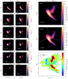 |
Fig. 10. Left: Hess diagrams in (MG, G − Ks) as derived from the data and predicted by the model (left to right) shown for the different horizontal slices. The height increases from top to bottom. The numbers of stars are given in brackets. Right: total Hess diagrams (top and middle) and their relative ratio (bottom). The white lines in the middle plot define the separation into the UMS, LMS, and RGB regions. |
We further investigated the UMS, LMS, and RGB populations separately. We defined them with the white lines in the middle plot of the right panel of Fig. 10. The border between the lower and upper parts of the MS approximately corresponds to the stellar masses of 1.5 M⊙. We plot two projections of the total Hess diagrams onto the magnitude and colour axis. The resulting colour distributions and luminosity functions are shown in the top and middle panels of Fig. 11. In addition to the general difference in the number of stars, we see more clearly that the modelled LMS is more peaked than the observed one, while the UMS and RGB regions are less pronounced in the model. The same information can be obtained from the individual vertical density laws plotted for the three populations (Fig. 11, bottom panel). The LMS, UMS, and RGB regions are under-populated in the model by 3.6%, 6%, and 34.7%, respectively.
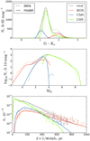 |
Fig. 11. UMS, LMS, and RGB stars studied separately. Top: colour distributions as observed and modelled for the whole local cylinder. Middle: luminosity functions for the same three populations. Bottom: stellar number densities as functions of observed height. The grey line corresponds to the red curve in Fig. 6. |
5. Discussion
In this section we discuss several potential problems of our modelling procedure. When we analyzed the Hess diagrams (Fig. 10), we found a few tenths of stars in the data that were clearly outliers (see the reddest and bluest G − Ks values). These might be misidentified stars as well as contamination of the metal-poor thick-disc and halo stars and objects with unrealistic metallicities, magnitudes, or colours. One of the problematic red areas is associated with the LMS region: the observed MS is noticeably wider than the predicted one. This might be caused by the impact of binarity, which is ignored in our modelling. Additionally, metal-rich stars are present in the data sample ([Fe/H] > 0.2), and their number is underestimated with the model AMR (see Fig. 16 in Paper I, the metallicity prescribed to the youngest stellar population is +0.02 dex). Moreover, we predict an underestimated stellar density in the RGB region. This we attribute to the simplicity of accounting for the SQ completeness factor, which is included in the modelling as a function of height above the plane (Fig. 2, top panel), although it also shows a variation with colour and absolute magnitude (Fig. 2, bottom panel). By ignoring this dependence of SQ on magnitude and colour, we may over- or underestimate stellar numbers in the regions of the Hess diagram where the values of incompleteness in Fig. 2 deviate considerably from the average. This effect can also be responsible for a blue region near the UMS at G − Ks ≈ 0.8 mag (compare to the bottom panel of Fig. 2). On the other hand, when considered together with a blue region in the LMS (see colour range 1.8 ≲ (G − Ks)/mag ≲ 2.8 at the relative ratio plot in Fig. 10), it points to a small colour shift between the modelled and observed Hess diagrams of ∼0.1 mag in G − Ks. Several reasons may be responsible for this: an underestimated reddening, a systematic shift of isochrones, or a lack of metal-poor thin-disc populations in the data due to an incorrect separation of thin- and thick-disc stars; the interplay of all these factors is also possible. Taking into account the locality of our volume, however, it is improbable that this shift is related to the underestimated reddening. We return to this question in view of the new results obtained on the basis of Gaia DR2 (see below). Furthermore, we discuss the sensitivity of our results to the choice of dust map and stellar library.
A possible unreliability of the dust map can have a twofold impact on our results. First, the predicted Hess diagram may appear shifted in the colour-magnitude plane relative to the observed one. Second, as the data selection function strongly depends on apparent magnitude and colour and the predicted number of stars may change significantly over the colour-magnitude bins (this is particularly related to the UMS and RGB regions), under- or overestimation of extinction and reddening may add up to the uncertainty in star counts. The 3D dust map used in our simulations is mainly based on the high-angular resolution extinction model from Green et al. (2015) constructed by the statistical technique from photometric data of Pan-STARRS and 2MASS. The safe range of distances covered by this map lies approximately in a range from 300 pc to 4–5 kpc, although the values of the minimum and maximum reliable distance may significantly vary over the sky. In most of our modelled sky region, the minimum reliable distance is ∼200 pc and extends to 300 pc. This implies that reddening may not be modelled reliably in those regions of the cylinder that are in close vicinity to the Sun. However, we do not expect the roughness of the extinction map in the nearby areas to have a significant effect on the modelling process because with the cut of |b| > 20°, we avoid the most problematic near-plane regions. To quantify the impact of the extinction model on our results, we tested an additional 3D reddening map from Capitanio et al. (2017)6 when we used Gaia DR2 data (see below).
With the full stellar evolution now included in the modelling, our predictions are sensitive to the choice of the stellar evolution package. To quantify the corresponding uncertainty, we tested an alternative set of isochrones generated by the PAdova and TRieste Stellar Evolution Code (PARSEC; Bressan et al. 2012, Marigo et al. 2017) for the same range of metallicities and ages as described in Sect. 3.3. The total number of predicted stars increased by ∼10%, but no appreciable difference of the model behaviour was discovered apart from this.
As the Gaia DR2 astrometry and completeness are significantly improved with respect to TGAS (Lindegren et al. 2018; Arenou et al. 2018) and the Gaia radial velocities have an even better precision than those of RAVE (Katz et al. 2018), we performed a sanity check complementary to the local test using the Gaia DR2 astrometric parameters and radial velocities. To mimic the test presented in this paper, we used the Gaia×RAVE cross-match with the Gaia radial velocities (Soubiran et al. 2018) and selected the local subset belonging to the same spatial volume and area on the sky as the TGAS×RAVE sample described in Sect. 2. We did not attempt to repeat the full forward-modelling described in Sect. 3.2 by accounting for parallax errors; instead, we used geometric distances from Bailer-Jones et al. (2018) derived in the framework of Bayesian approach on the basis of Gaia DR2 parallaxes. In this test we did not apply metallicity scatter to the AMR either, which allowed us to reduce the number of stellar assemblies and speed up the calculations. These simplifications do not influence the star counts much: (1) even if the distance errors reach ∼50% for the individual stars at 1 kpc, the overall stellar density at this heliocentric distance is quite low in our geometry, and the corresponding uncertainty introduced in the number of stars in the volume is not significant; and (2) the metallicity grid affects the modelled number of stars only indirectly through the sample selection function, which is sensitive to the apparent magnitudes and colours. In order to avoid additional incompleteness, no cuts on RAVE Fe or Mg abundances were used. Correspondingly, the thick disc was added to the model as a mono-age population with a metallicity of −0.7 dex and a Gaussian dispersion of 0.2 dex. As some stars of the RAVE DR5 are missing in the Gaia×RAVE cross-match (because of unknown Gaia radial velocities or match problems; this makes up ∼11% of the full RAVE DR5), we built a modified RAVE selection function that incorporates this additional incompleteness and used it for our test. The selected Gaia×RAVE local sample contains 63 408 stars. We built absolute and apparent Hess diagrams using the updated Gaia DR2 G-band and GBP − GRP colour from PARSEC isochrones. Because the metallicity scatter and distance errors were not modelled, all features of the predicted Hess diagram look more pronounced than those seen in the data (Fig. 12). Regardless of the width of the observed and modelled MS, we expect their centres to coincide; however, the right panel of Fig. 12 shows that this is not the case, which implies a small colour shift of about ∼0.05 mag in GBP − GRP between the data and the model. As the thick disc is included at this stage, the shift is most likely related to a systematic shift of the isochrones. We also observe an excess of stars in the UMS region, which indicates that a better understanding of the Gaia selection function is necessary. Additionally, there is a deficit of stars in the modelled LMS in the colour range of 1.7 ≲ (GBP − GRP)/mag ≲ 1.9. As we did not include any special colour cuts and the applied selection function is essentially independent of colour, this feature must arise from the stellar library and needs to be further investigated in future work. With this setup we reproduced star counts with an accuracy of ∼3%. We report the presence of non-reproduced dynamically cold populations at |z|< 100 pc even more confidently than in case of the TGAS×RAVE test (Fig. 13, also see the upper left panel of Fig. 8). Finally, we compared the outcome of the sanity check star counts for the Bovy et al. (2016) and Capitanio et al. (2017) dust maps. We find only a difference between the two runs of ∼1%. Thus, the outcome of our tests gives us a good insight into potential problems of the model and can be viewed as a first step to the future and more comprehensive work with Gaia DR2.
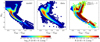 |
Fig. 12. Modelled (left) and observed (middle) absolute Hess diagrams of the the stars in common between RAVE and Gaia DR2. The right panel displays their relative ratio. The sample belongs to the solar cylinder of 300 pc radius and 1 kpc height below the midplane with stars selected in the sky area of the TGAS×RAVE sample (see Sect. 2.1 and Fig. 1). The thick disc is included in the modelling. Model and data are both smoothed with a window of 0.04 × 0.2 mag2 (2 × 2 bins in (GBP − GRP, MG)). |
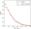 |
Fig. 13. Normalised |W|-velocity distribution function at |z|< 100 pc. The data sample is based on Gaia DR2. |
6. Conclusions
We used the forward-modelling technique to test the semi-analytic JJ model. We selected a clean sample of thin-disc stars from the TGAS×RAVE cross-match providing precise astrometry as well as radial velocities and chemical abundances. We investigated the large local volume of the solar cylinder with radius of 300 pc extending to 1 kpc below the Galactic plane. The full stellar evolution in the form of MIST stellar isochrones was implemented in the model. For each modelled height z, we accounted for the parallax errors and reddening, and reproduced the incompleteness of the sample. The results were assigned with the additional weights to model the effect of the distance error in the vertical direction.
We found that the model predictions and data agree well with each other. A deviation of ∼1σ is found between the modelled and observed velocity distribution functions f(|W|) close to the Galactic plane, indicating that the role of the cold young stellar populations may be underestimated in our local disc model. When complemented with the velocity distribution functions for the different magnitude bins of the MS stars, this implies that the source of the discrepancy in vertical kinematics is related to the lower part of the UMS region. A complementary test based on the RAVE and new Gaia DR2 data confirmed the results presented in Sect. 4, and the reported underestimation of dynamically cold populations is even more prominent when tested with Gaia DR2 astrometry and radial velocities.
With this realistic performance test, we demonstrated the robustness of the local JJ model when compared to the data up to 1 kpc away from the Galactic plane. However, non-negligible deviations from the data are identified in case of the vertical kinematics of the disc, which suggests that the model should be adapted to match the new Gaia data. The next step will include an extension of the model to other Galactocentric distances: the code Chempy will be used to build the chemical evolution model of the disc, consistent with the adopted SFR and AVR varying with Galactic radius. For this purpose, Gaia DR2 and its next releases as well as high-resolution spectroscopic surveys such as APOGEE, Gaia-ESO, and GALAH will be of high benefit.
The cross-match between catalogues was performed by the RAVE Collaboration, see https://www.rave-survey.org/downloads
Acknowledgments
This work was supported by Sonderforschungsbereich SFB 881 “The Milky Way System” (subprojects A6 and A5) of the German Research Foundation (DFG). Funding for RAVE has been provided by the Australian Astronomical Observatory, the Leibniz-Institut für Astrophysik Potsdam (AIP), the Australian National University, the Australian Research Council, the French National Research Agency, the German Research Foundation (SPP 1177 and SFB 881), the European Research Council (ERC-StG 240271 Galactica); the Istituto Nazionale di Astrofisica at Padova, The Johns Hopkins University, the National Science Foundation of the USA (AST-0908326), the W. M. Keck foundation, the Macquarie University, the Netherlands Research School for Astronomy, the Natural Sciences and Engineering Research Council of Canada, the Slovenian Research Agency, the Swiss National Science Foundation, the Science & Technology Facilities Council of the UK, Opticon, the Strasbourg Observatory, and the Universities of Groningen, Heidelberg, and Sydney. The RAVE web site is at http://www.rave-survey.org. This work has made use of data from the European Space Agency (ESA) mission Gaia (https://www.cosmos.esa.int/gaia), processed by the Gaia Data Processing and Analysis Consortium (DPAC, https://www.cosmos.esa.int/web/gaia/dpac/consortium). Funding for the DPAC has been provided by national institutions, in particular the institutions participating in the Gaia Multilateral Agreement.
References
- Arenou, F., Luri, X., Babusiaux, C., et al. 2018, A&A, 616, A17 [Google Scholar]
- Bailer-Jones, C. A. L., Rybizki, J., Fouesneau, M., Mantelet, G., & Andrae, R. 2018, AJ, 156, 58 [NASA ADS] [CrossRef] [Google Scholar]
- Bovy, J. 2017, MNRAS, 470, 1360 [NASA ADS] [CrossRef] [Google Scholar]
- Bovy, J., Rix, H.-W., Green, G. M., Schlafly, E. F., & Finkbeiner, D. P. 2016, ApJ, 818, 130 [NASA ADS] [CrossRef] [Google Scholar]
- Bovy, J., Rix, H.-W., & Hogg, D. W. 2012a, ApJ, 751, 131 [NASA ADS] [CrossRef] [Google Scholar]
- Bovy, J., Rix, H.-W., Liu, C., et al. 2012b, ApJ, 753, 148 [NASA ADS] [CrossRef] [Google Scholar]
- Bressan, A., Marigo, P., Girardi, L., et al. 2012, MNRAS, 427, 127 [NASA ADS] [CrossRef] [Google Scholar]
- Capitanio, L., Lallement, R., Vergely, J. L., Elyajouri, M., & Monreal-Ibero, A. 2017, A&A, 606, A65 [NASA ADS] [CrossRef] [EDP Sciences] [Google Scholar]
- Carrasco, J. M., Evans, D. W., Montegriffo, P., et al. 2016, A&A, 595, A7 [NASA ADS] [CrossRef] [EDP Sciences] [Google Scholar]
- Choi, J., Dotter, A., Conroy, C., et al. 2016, ApJ, 823, 102 [NASA ADS] [CrossRef] [Google Scholar]
- Czekaj, M. A., Robin, A. C., Figueras, F., Luri, X., & Haywood, M. 2014, A&A, 564, A102 [NASA ADS] [CrossRef] [EDP Sciences] [Google Scholar]
- Dotter, A. 2016, ApJS, 222, 8 [NASA ADS] [CrossRef] [Google Scholar]
- Drimmel, R., Cabrera-Lavers, A., & López-Corredoira, M. 2003, A&A, 409, 205 [NASA ADS] [CrossRef] [EDP Sciences] [Google Scholar]
- Eisenstein, D. J., Weinberg, D. H., Agol, E., et al. 2011, AJ, 142, 72 [Google Scholar]
- Gaia Collaboration (Brown, A. G. A., et al.) 2016a, A&A, 595, A2 [NASA ADS] [CrossRef] [EDP Sciences] [Google Scholar]
- Gaia Collaboration (Prusti, T., et al.) 2016b, A&A, 595, A1 [NASA ADS] [CrossRef] [EDP Sciences] [Google Scholar]
- Gaia Collaboration (Brown, A. G. A., et al.) 2018, A&A, 616, A1 [NASA ADS] [CrossRef] [EDP Sciences] [Google Scholar]
- Gao, S., Just, A., & Grebel, E. K. 2013, A&A, 549, A20 [NASA ADS] [CrossRef] [EDP Sciences] [Google Scholar]
- Gilmore, G., Randich, S., Asplund, M., et al. 2012, The Messenger, 147, 25 [NASA ADS] [Google Scholar]
- Girardi, L. 2016, Astron. Nachr., 337, 871 [NASA ADS] [CrossRef] [Google Scholar]
- Girardi, L., Groenewegen, M. A. T., Hatziminaoglou, E., & da Costa, L. 2005, A&A, 436, 895 [NASA ADS] [CrossRef] [EDP Sciences] [Google Scholar]
- Green, G. M., Schlafly, E. F., Finkbeiner, D. P., et al. 2015, ApJ, 810, 25 [NASA ADS] [CrossRef] [Google Scholar]
- Grisoni, V., Spitoni, E., & Matteucci, F. 2018, MNRAS, 481, 2570 [NASA ADS] [Google Scholar]
- Grisoni, V., Spitoni, E., Matteucci, F., et al. 2017, MNRAS, 472, 3637 [NASA ADS] [CrossRef] [Google Scholar]
- Hayden, M. R., Recio-Blanco, A., de Laverny, P., Mikolaitis, S., & Worley, C. C. 2017, A&A, 608, L1 [NASA ADS] [CrossRef] [EDP Sciences] [Google Scholar]
- Haywood, M., Di Matteo, P., Lehnert, M. D., Katz, D., & Gómez, A. 2013, A&A, 560, A109 [NASA ADS] [CrossRef] [EDP Sciences] [Google Scholar]
- Henden, A. A., Welch, D. L., Terrell, D., & Levine, S. E. 2009, AAS Meeting. Abstr., 214, 669 [Google Scholar]
- Høg, E., Fabricius, C., Makarov, V. V., et al. 2000, A&A, 355, L27 [Google Scholar]
- Jahreiß, H., & Wielen, R. 1997, in HIPPARCOS’97, Presentation of the Hipparcos and Tycho Catalogues and the First Astrophysical Results of the Hipparcos Space Astrometry Mission, eds. B. Battrick, M. A. C. Perryman, & P. L. Bernacca (Noordwijk: ESA), ESA SP-402, 675 [Google Scholar]
- Jordi, C., Gebran, M., Carrasco, J. M., et al. 2010, A&A, 523, A48 [NASA ADS] [CrossRef] [EDP Sciences] [Google Scholar]
- Just, A., & Jahreiß, H. 2010, MNRAS, 402, 461 [NASA ADS] [CrossRef] [Google Scholar]
- Just, A., & Rybizki, J. 2016, Astron. Nachr., 337, 880 [NASA ADS] [CrossRef] [Google Scholar]
- Just, A., Gao, S., & Vidrih, S. 2011, MNRAS, 411, 2586 [NASA ADS] [CrossRef] [Google Scholar]
- Just, A., Sysoliatina, K., & Koutsouridou, I. 2018, in IAU Symp., 330, eds. A. Recio-Blanco, P. de Laverny, A. G. A. Brown, & T. Prusti, 168 [NASA ADS] [Google Scholar]
- Katz, D., Sartoretti, P., Cropper, M., et al. 2018, A&A, submitted [arXiv:1804.09372] [Google Scholar]
- Kordopatis, G., Gilmore, G., Steinmetz, M., et al. 2013, AJ, 146, 134 [NASA ADS] [CrossRef] [Google Scholar]
- Kunder, A., Kordopatis, G., Steinmetz, M., et al. 2017, AJ, 153, 75 [NASA ADS] [CrossRef] [Google Scholar]
- Lindegren, L., Lammers, U., Bastian, U., et al. 2016, A&A, 595, A4 [NASA ADS] [CrossRef] [EDP Sciences] [Google Scholar]
- Lindegren, L., Hernández, J., Bombrun, A., et al. 2018, A&A, 616, A2 [NASA ADS] [CrossRef] [EDP Sciences] [Google Scholar]
- Luo, A.-L., Zhao, Y.-H., Zhao, G., et al. 2015, Res. Astron. Astrophys., 15, 1095 [NASA ADS] [CrossRef] [Google Scholar]
- Marigo, P., Girardi, L., Bressan, A., et al. 2017, ApJ, 835, 77 [NASA ADS] [CrossRef] [Google Scholar]
- Marshall, D. J., Robin, A. C., Reylé, C., Schultheis, M., & Picaud, S. 2006, A&A, 453, 635 [NASA ADS] [CrossRef] [EDP Sciences] [Google Scholar]
- Martell, S. L., Sharma, S., Buder, S., et al. 2017, MNRAS, 465, 3203 [NASA ADS] [CrossRef] [Google Scholar]
- Michalik, D., Lindegren, L., & Hobbs, D. 2015, A&A, 574, A115 [NASA ADS] [CrossRef] [EDP Sciences] [Google Scholar]
- Munari, U., Henden, A., Frigo, A., et al. 2014, AJ, 148, 81 [NASA ADS] [CrossRef] [Google Scholar]
- Nordström, B., Mayor, M., Andersen, J., et al. 2004, A&A, 418, 989 [NASA ADS] [CrossRef] [EDP Sciences] [Google Scholar]
- Paxton, B., Bildsten, L., Dotter, A., et al. 2011, ApJS, 192, 3 [Google Scholar]
- Paxton, B., Cantiello, M., Arras, P., et al. 2013, ApJS, 208, 4 [NASA ADS] [CrossRef] [Google Scholar]
- Paxton, B., Marchant, P., Schwab, J., et al. 2015, ApJS, 220, 15 [Google Scholar]
- Robin, A. C., Reylé, C., Derrière, S., & Picaud, S. 2003, A&A, 409, 523 [NASA ADS] [CrossRef] [EDP Sciences] [Google Scholar]
- Robin, A. C., Reylé, C., Marshall, D. J., & Schultheis, M. 2012, Astrophys. Space Sci. Proc., 26, 171 [NASA ADS] [CrossRef] [Google Scholar]
- Robin, A. C., Bienaymé, O., Fernández-Trincado, J. G., & Reylé, C. 2017, A&A, 605, A1 [NASA ADS] [CrossRef] [EDP Sciences] [Google Scholar]
- Röser, S., Schilbach, E., Schwan, H., et al. 2008, A&A, 488, 401 [NASA ADS] [CrossRef] [EDP Sciences] [Google Scholar]
- Rybizki, J., & Just, A. 2015, MNRAS, 447, 3880 [NASA ADS] [CrossRef] [Google Scholar]
- Rybizki, J., Just, A., & Rix, H.-W. 2017, A&A, 605, A59 [NASA ADS] [CrossRef] [EDP Sciences] [Google Scholar]
- Schlegel, D. J., Finkbeiner, D. P., & Davis, M. 1998, ApJ, 500, 525 [NASA ADS] [CrossRef] [Google Scholar]
- Schönrich, R., Binney, J., & Dehnen, W. 2010, MNRAS, 403, 1829 [NASA ADS] [CrossRef] [Google Scholar]
- Sharma, S., Bland-Hawthorn, J., Johnston, K. V., & Binney, J. 2011, Astrophysics Source Code Library [record ascl:1101.007] [Google Scholar]
- Skrutskie, M. F., Cutri, R. M., Stiening, R., et al. 2006, AJ, 131, 1163 [NASA ADS] [CrossRef] [Google Scholar]
- Soubiran, C., Jasniewicz, G., Chemin, L., et al. 2018, A&A, 616, A7 [NASA ADS] [CrossRef] [EDP Sciences] [Google Scholar]
- Steinmetz, M., Zwitter, T., Siebert, A., et al. 2006, AJ, 132, 1645 [NASA ADS] [CrossRef] [Google Scholar]
- Sysoliatina, K., Just, A., Golubov, O., et al. 2018, A&A, 614, A63 [Google Scholar]
- van Leeuwen, F. 2007, in Hipparcos, the New Reduction of the Raw Data, Astrophysics and Space Science Library, 350 [Google Scholar]
- van Leeuwen, F., Evans, D. W., De Angeli, F., et al. 2017, A&A, 599, A32 [NASA ADS] [CrossRef] [EDP Sciences] [Google Scholar]
- Vergely, J.-L., Ferrero, R. F., Egret, D., & Koeppen, J. 1998, A&A, 340, 543 [NASA ADS] [Google Scholar]
- Wojno, J., Kordopatis, G., Steinmetz, M., et al. 2016, MNRAS, 461, 4246 [NASA ADS] [CrossRef] [Google Scholar]
- Wojno, J., Kordopatis, G., Piffl, T., et al. 2017, MNRAS, 468, 3368 [NASA ADS] [CrossRef] [Google Scholar]
- Zacharias, N., Finch, C., & Frouard, J. 2017, AJ, 153, 166 [NASA ADS] [CrossRef] [Google Scholar]
All Figures
|
Fig. 1. Sky coverage of the data in the Galactic coordinates. The full TGAS×RAVE cross-match is shown in grey. The selected thin-disc sample (blue) lies below the Galactic plane; its special shape at b < −50° reflects the Gaia scanning law pattern. |
| In the text | |
|
Fig. 2. Top: fraction of stars missing in the solar cylinder of 300 pc radius and 1 kpc height below the midplane. The orange line corresponds to the contribution from the low-quality stars, and the green curve gives an upper limit on the fraction of stars that did not enter the final sample because of the missing chemical abundances. The total fraction of missing stars is shown in blue. Bottom: total fraction of the missing stars as a function of absolute G magnitude and G − Ks colour. |
| In the text | |
|
Fig. 3. Theoretical HR diagrams for the thin disc as predicted by the local JJ model with the use of MIST isochrones. Five age bins illustrate the contributions from the different thin-disc populations to the total HR diagram (lower right). The blue box roughly corresponds to the region studied in this work. |
| In the text | |
|
Fig. 4. Normalised parallax error PDF as taken from the full TGAS×RAVE cross-match (black). The orange, yellow, and violet histograms correspond to the PDFs of the subsamples with different distance ranges. The similarity of their shapes demonstrates an independence of the parallax error from the parallax itself (i.e. the distance). In the inset an example normalised Gaussian PDF for the observed parallax is plotted. The true parallax and its observational error are set to 1 and 0.3 mas, respectively. |
| In the text | |
|
Fig. 5. Top: mean observed heliocentric distance |
| In the text | |
|
Fig. 6. Top: volume number density of stars in the modelled cylinder. The blue line represents the data, and violet and red curves are the model predictions before and after the vertical error effect is taken into account. Middle: cumulative number of stars in the cylinder as a function of observed height |
| In the text | |
|
Fig. 7. Normalised parallax distributions as derived from the TGAS×RAVE thin-disc sample and as predicted by the JJ model. |
| In the text | |
|
Fig. 8. Normalised velocity distribution functions f(|W|) for the six horizontal slices (3 × 2 plots on the left). The right graph shows f(|W|) for the whole modelled cylinder. |
| In the text | |
|
Fig. 9. Normalised velocity distribution functions f(|W|) for the different MV cuts. The selection of the MS stars and separation into magnitude bins is shown on the right, where the CMD of the full TGAS×RAVE thin-disc sample is plotted with APASS photometry and the RAVE metallicity is colour-coded. |
| In the text | |
|
Fig. 10. Left: Hess diagrams in (MG, G − Ks) as derived from the data and predicted by the model (left to right) shown for the different horizontal slices. The height increases from top to bottom. The numbers of stars are given in brackets. Right: total Hess diagrams (top and middle) and their relative ratio (bottom). The white lines in the middle plot define the separation into the UMS, LMS, and RGB regions. |
| In the text | |
|
Fig. 11. UMS, LMS, and RGB stars studied separately. Top: colour distributions as observed and modelled for the whole local cylinder. Middle: luminosity functions for the same three populations. Bottom: stellar number densities as functions of observed height. The grey line corresponds to the red curve in Fig. 6. |
| In the text | |
|
Fig. 12. Modelled (left) and observed (middle) absolute Hess diagrams of the the stars in common between RAVE and Gaia DR2. The right panel displays their relative ratio. The sample belongs to the solar cylinder of 300 pc radius and 1 kpc height below the midplane with stars selected in the sky area of the TGAS×RAVE sample (see Sect. 2.1 and Fig. 1). The thick disc is included in the modelling. Model and data are both smoothed with a window of 0.04 × 0.2 mag2 (2 × 2 bins in (GBP − GRP, MG)). |
| In the text | |
|
Fig. 13. Normalised |W|-velocity distribution function at |z|< 100 pc. The data sample is based on Gaia DR2. |
| In the text | |
Current usage metrics show cumulative count of Article Views (full-text article views including HTML views, PDF and ePub downloads, according to the available data) and Abstracts Views on Vision4Press platform.
Data correspond to usage on the plateform after 2015. The current usage metrics is available 48-96 hours after online publication and is updated daily on week days.
Initial download of the metrics may take a while.