| Issue |
A&A
Volume 620, December 2018
|
|
|---|---|---|
| Article Number | A39 | |
| Number of page(s) | 15 | |
| Section | Extragalactic astronomy | |
| DOI | https://doi.org/10.1051/0004-6361/201833055 | |
| Published online | 27 November 2018 | |
Impact of metallicity and star formation rate on the time-dependent, galaxy-wide stellar initial mass function⋆
1
European Southern Observatory, Karl-Schwarzschild-Straße 2, 85748 Garching bei München, Germany
e-mail: This email address is being protected from spambots. You need JavaScript enabled to view it.
2
Helmholtz Institut für Strahlen und Kernphysik, Universität Bonn, Nussallee 14-16, 53115 Bonn, Germany
3
Astronomical Institute, Charles University in Prague, V Holešovičkách 2, 180 00 Praha 8, Czech Republic
4
Department of Physics, Institute for Advanced Studies in Basic Sciences (IASBS), PO Box 11365-9161, Zanjan, Iran
5
Instituto de Astrofísica de Canarias, 38200 La Laguna, Tenerife, Spain
6
Institute for Astronomy, University of Edinburgh, Blackford Hill, EH9 3HJ Edinburgh, UK
Received:
20
March
2018
Accepted:
24
August
2018
Abstract
The stellar initial mass function (IMF) is commonly assumed to be an invariant probability density distribution function of initial stellar masses. These initial stellar masses are generally represented by the canonical IMF, which is defined as the result of one star formation event in an embedded cluster. As a consequence, the galaxy-wide IMF (gwIMF) should also be invariant and of the same form as the canonical IMF; gwIMF is defined as the sum of the IMFs of all star-forming regions in which embedded clusters form and spawn the galactic field population of the galaxy. Recent observational and theoretical results challenge the hypothesis that the gwIMF is invariant. In order to study the possible reasons for this variation, it is useful to relate the observed IMF to the gwIMF. Starting with the IMF determined in resolved star clusters, we apply the IGIMF-theory to calculate a comprehensive grid of gwIMF models for metallicities, [Fe/H] ∈ (−3, 1), and galaxy-wide star formation rates (SFRs), SFR ∈ (10−5, 105) M⊙ yr−1. For a galaxy with metallicity [Fe/H] < 0 and SFR > 1 M⊙ yr−1, which is a common condition in the early Universe, we find that the gwIMF is both bottom light (relatively fewer low-mass stars) and top heavy (more massive stars), when compared to the canonical IMF. For a SFR < 1 M⊙ yr−1 the gwIMF becomes top light regardless of the metallicity. For metallicities [Fe/H] > 0 the gwIMF can become bottom heavy regardless of the SFR. The IGIMF models predict that massive elliptical galaxies should have formed with a gwIMF that is top heavy within the first few hundred Myr of the life of the galaxy and that it evolves into a bottom heavy gwIMF in the metal-enriched galactic centre. Using the gwIMF grids, we study the SFR−Hα relation and its dependency on metallicity and the SFR. We also study the correction factors to the Kennicutt SFRK − Hα relation and provide new fitting functions. Late-type dwarf galaxies show significantly higher SFRs with respect to Kennicutt SFRs, while star-forming massive galaxies have significantly lower SFRs than hitherto thought. This has implications for gas-consumption timescales and for the main sequence of galaxies. We explicitly discuss Leo P and ultra-faint dwarf galaxies.
Key words: galaxies: stellar content / stars: luminosity function, mass function / galaxies: elliptical and lenticular, cD / galaxies: star formation / galaxies: dwarf / stars: formation
The IGIMF grid is only available at the CDS via anonymous ftp to cdsarc.u-strasbg.fr (130.79.128.5) or via http://cdsarc.u-strasbg.fr/viz-bin/qcat?J/A+A/620/A39
© ESO 2018
1. Introduction
The stellar initial mass function (IMF) is a theoretical representation of the number distribution of stellar masses at the births of stars formed in one star formation event. The IMF is often described as ξ⋆(m) = dN/dm, where dN is the number of stars formed locally1 in the mass interval m to m+dm. The IMF can be mathematically expressed conveniently in the form of a multi-power law with indices  for stars in the mass range 0.1–0.5 M⊙ and
  for stars more massive than 0.5 M⊙. The fact that this canonical stellar IMF is an invariant probability density distribution function of stellar masses is usually considered to be a null hypothesis and a benchmark for stellar population studies (e.g. Selman & Melnick 2008; Kroupa et al. 2013; Offner et al. 2014; Jeřábková et al. 2017; Kroupa & Jerabkova 2018).
The detailed form of the IMF is relevant for almost all fields related to star formation, thus it has important implications for the luminous, dynamical, and chemical evolution of stellar populations. In studies of both Galactic and extragalactic integrated systems, an IMF needs to be assumed to derive star formation rates (SFRs) by extrapolating from massive stars that always dominat luminosities. The IMF is therefore a fundamental entity entering directly or indirectly into many astrophysical problems (e.g. Kroupa 2002; Chabrier 2003; Bastian et al. 2010; Kroupa et al. 2013; Offner et al. 2014; Hopkins 2018). Observational studies of nearby star-forming regions suggest that stars form in dense cores inside molecular clouds (Lada & Lada 2003; Lada 2010; Kirk & Myers 2011, 2012; Gieles et al. 2012; Megeath et al. 2016; Stephens et al. 2017; Ramírez Alegría et al. 2016; Hacar et al. 2017a; Lucas et al. 2018) usually following the canonical stellar IMF (e.g. Kroupa 2002; Chabrier 2003; Bastian et al. 2010; Kroupa et al. 2013).
The canonical stellar IMF is derived from observations of field stars and nearby star-forming regions that form stars in local over-densities called embedded star clusters or correlated star formation events (CSFEs), which are approximately 1 pc across and form a population of stars on a timescale of 1 Myr (Kroupa et al. 2013; Yan et al. 2017 and references therein). The molecular clouds as a whole are not self-gravitationally bound in the majority of cases (Hartmann et al. 2001; Elmegreen 2002, 2007; Ballesteros-Paredes et al. 2007; Dobbs et al. 2011; Lim et al. 2018). However, their complex filamentary substructures on sub-parsec scales can be locally gravitationally bound and also gravitationally unstable (Hacar et al. 2017a,b), which may set the initial conditions for the formation of stars. Star formation happens in correlated dense regions of molecular gas, which have intrinsic physical connections instead of being distributed randomly inside molecular clouds (e.g. Joncour et al. 2018). For practical purposes we refer to these CSFEs as embedded clusters. For the computations of gwIMF only the stellar census matters. Nevertheless the initial conditions in star-forming regions are relevant to interpret observations of stellar populations in galaxies. The CSFEs and embedded clusters are potentially dynamically very active (Kroupa & Boily 2002; Kroupa et al. 2005; Oh et al. 2015; Oh & Kroupa 2016; Brinkmann et al. 2017)2. Thus they spread their stars out through the star-forming regions and later to the galactic field very quickly within fractions of a Myr. Therefore, the dynamical processes on a star cluster scale need to be taken into account to obtain a physically correct picture of young stellar populations and of their distribution.
Increasing observational evidence suggests that star formation is a self-regulated process rather than a purely stochastic process (Papadopoulos 2010; Kroupa et al. 2013; Kroupa 2015; Yan et al. 2017; Lim et al. 2018; Plunkett et al. 2018). The idea that the star formation efficiency of embedded clusters is found, both observationally and theoretically, to be less than 30–40% (Adams & Fatuzzo 1996; Lada & Lada 2003; Lada 2010; Hansen et al. 2012; Machida & Matsumoto 2012; Federrath et al. 2014; Federrath 2015; Megeath et al. 2016) supports self-regulation. The gravitational collapse of an embedded-cluster forming cloud core leads to star formation that heats, ionizes, and removes gas from the core. This may be one reason why a relation between a most massive star and an embedded cluster mass might exist (Weidner et al. 2010).
For nearby resolved star-forming regions, the IMF can be understood as describing a single star formation event happening on a physical scale of about 1 pc and beyond this scale the molecular gas is gravitationally unstable and would form individual embedded clusters or small groups of stars. However, it is non-trivial to calculate the IMF of an unresolved stellar population, for example, of a whole galaxy because it contains many stellar clusters formed at different times. The galaxy-wide IMF (gwIMF) is, on the other hand, the sum of all the IMFs of all star-forming regions belonging to a given galaxy (e.g. Kroupa & Weidner 2003; Weidner et al. 2013b; Kroupa et al. 2013; Yan et al. 2017, see also Fig. 1). Assuming that the canonical IMF is a universal probability density distribution function, the shape of the gwIMF should be equal to that of the canonical IMF. On the other hand, if the gwIMF differs from the canonical IMF, then the canonical IMF cannot be universal and/or it cannot be described as a stationary probability density distribution function.
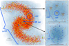 |
Fig. 1. Schematic showing a late-type galaxy. Its field population is represented by red and orange stars. The newly formed stellar population is indicated by coloured circles that represent CSFEs (embedded star clusters). The colours and sizes of symbols scale with stellar/cluster mass. The acronyms from Table 3 are shown here with examples. Right bottom panel: a young massive embedded cluster, which will most likely survive and contribute to the open star cluster population of the galaxy. Right top panel: young embedded cluster complex composed of a number of low-mass embedded clusters, which will evolve into a T Tauri association once the embedded clusters expand after loss of their residual gas and disperse into the galaxy field stellar population. |
Therefore, a fundamental question naturally arises: Is the stellar IMF a universal probability density distribution function (Kroupa et al. 2013)? An overabundance of low-mass stars (<1 M⊙) with respect to the canonical stellar IMF is called a “bottom-heavy” IMF and a deficit of low-mass stars is a “bottom-light” IMF. For the massive stars (>1 M⊙), an overabundance or deficit of stars relative to the canonical IMF results in a “top-heavy” and a “top-light” IMF, respectively. Studies of globular clusters, ultra-compact dwarf galaxies, and young massive clusters have suggested that in a low metallicity and high gas-density environment the stellar IMF may become top heavy (e.g. Dabringhausen et al. 2009, 2012; Marks et al. 2012; Zonoozi et al. 2016; Haghi et al. 2017; Kalari et al. 2018; Schneider et al. 2018), while being bottom heavy in metal-rich (Z > Z⊙) environments (Kroupa 2002; Marks & Kroupa 2012). Such bottom-heavy IMFs have been found in the centre of nearby elliptical galaxies, where the metallicities are higher than Z⊙ (van Dokkum & Conroy 2010; Conroy et al. 2017). The progenitors of elliptical galaxies, on the other hand, have been suggested to have had top-heavy gwIMFs based on the evolution of their chemical composition (Matteucci 1994; Vazdekis et al. 1997; Weidner et al. 2013b; Ferreras et al. 2015; Martín-Navarro 2016). Top-heavy gwIMFs are often found in galaxies with high SFRs (Gunawardhana et al. 2011; Fontanot & De Lucia 2017; De Masi et al. 2018; Zhang et al. 2018; Fontanot et al. 2018a,b), while top-light gwIMFs are evident in galaxies with low SFRs (e.g. Lee et al. 2009; Meurer et al. 2009; Watts et al. 2018). The new method of tracing the variation of the gwIMF using observations of CNO isotopes in the molecular ISM with ALMA is interesting in this context and shows highly consistent results with the gwIMF theory (Papadopoulos 2010; Romano et al. 2017; Zhang et al. 2018). All this work suggests that gwIMF is not in a constant form and that it deviates from the canonical IMF, depending on star formation activity. These new findings challenge the idea that the IMF is a universal probability density distribution function.
We study the variation of the gwIMF using the integrated galaxy-wide IMF (IGIMF) theory (Kroupa & Weidner 2003; Kroupa et al. 2013; Yan et al. 2017). In this theory, the model of the gwIMF, i.e. the IGIMF, is constructed by summing (i.e. integrating) the IMFs of all star formation events in the whole galaxy at a given time. This results in a dependency of the gwIMF on the galaxy-wide SFR and metallicity and therefore also on the time.
With this contribution we investigate the full range of IGIMF variation. The novel aspect is the incorporation of the metallicity dependence of the IMF, as deduced by Marks et al. (2012) based on a stellar-dynamical study of evolved globular clusters, which also took into account constraints from ultra-compact dwarf galaxies by Dabringhausen et al. (2009), Dabringhausen et al. (2010, 2012). These constraints on how the IMF varies with local physical conditions are independent from any variation of the gwIMF deduced from observation. Thus, if the observed variation of the gwIMF can be accounted for with these IMF variations then this will play an important role in the convergence of our understanding of stellar populations over cosmic time.
Section 2 defines and clarifies terminology used in the paper. Section 3 explains the IGIMF theory and its implementations. In Sect. 4, we present our results by introducing a parametrized grid of gwIMFs. The implications include the evolution of the gwIMF in elliptical galaxies, quantifying the correction factors for Hα-based SFR estimators, the case of the Leo P dwarf galaxy and its very low SFR and massive star population, the baryonic Tully-Fisher relation (BTFR), and ultra-faint dwarf (UFD) galaxy satellites. In Sect. 5 additional discussion is provided and Sect. 6 contains the conclusions. We emphasize that this is the first time that a full grid of IGIMFs, with dependency on the galaxy-wide SFR and galaxy metallicity, has been made available.
2. Terminology
In the manuscript we frequently use four acronyms referring to the stellar initial mass function, i.e. IMF, cIMF, gwIMF, and IGIMF. The IMF represents the stellar initial mass function of stars formed during one star formation event in an initially gravitationally collapsing region in a molecular cloud (timescale ≈1 Myr, spatial scale ≈1 pc), that is in an embedded cluster. The cIMF represents the sum of the IMFs over a larger region, such as whole T Tauri and OB associations or even a larger part of a galaxy. The gwIMF is the initial stellar mass function of newly formed stars in a whole galaxy formed over a timescale δt ≈ 10 Myr (see Sect. 3.2) and can be inferred from observations or can be computed. The IGIMF is the theoretical framework that allows us to compute the gwIMF. For clarity the acronyms are summarized in Table 1. We use the term cIGIMF to refer to a theoretical formulation of the cIMF within the IGIMF framework. Once the region of interest is bigger than several molecular clouds (about >100 pc) the timescale δt would not change since the lifetime of molecular clouds is about 10 Myr.
Initial mass function acronyms summary.
We emphasize that it is important to distinguish between the IMF, cIMF, and gwIMF. This is because only if the star formation process is stochastically invariant, in the sense that once stars begin to form then the mass of the star is not related to the local physical conditions, will the IMF be an invariant probability density distribution function. If however, the mass of the born star (which assembles to within about 95% of its main-sequence value within about 105 yr, Wuchterl & Tscharnuter 2003; Duarte-Cabral et al. 2013) depends on the local conditions, then the IMF is not an invariant probability density distribution function. If the physical conditions in a embedded-cluster-forming molecular cloud core differ from those in another molecular cloud core, then the distribution of stellar masses also differ. The recent ALMA observation of an extremely young embedded cluster shows the millimetre sources to be nearly perfectly mass-segregated, suggesting that local physical conditions are probably very important in determining which stars form (Plunkett et al. 2018). A variation of the IMF with physical conditions has been expected from basic theory (see e.g. the discussion in Kroupa et al. 2013), but resolved observations of star-forming regions in the Local Group have been indicating that the variations, if they exist, are not detectable (Kroupa 2001, 2002; Bastian et al. 2010).
Thus, if the IMF is not an invariant probability density distribution function, then the sum of two star-forming events is not the same as a larger event with the same number of stars. The composite and galaxy-wide IMF in this case differs from the IMF. An explicit observational example of this is reported for the Orion A cloud by Hsu et al. (2012). The physical and empirical evidence thus suggests that the gwIMF should vary. The alternative, benchmark conservative model is to treat the IMF as a scale-free invariant probability density distribution function and to set gwIMF=stellar IMF taking into account the appropriate normalization. This conservative hypothesis is referred to as the caninvgwIMF hypothesis according to which gwIMF is equal in form to the invariant canonical stellar IMF.
3. Methods
The IGIMF theory is based on several assumptions that are described below in detail. We consider possible variations resulting in several different formulations that are all considered in this work. The assumptions, or axioms, are also detailed in Recchi & Kroupa (2015).
In a nutshell, the IGIMF theory spatially integrates over the whole galaxy by summing the local galactic star-forming regions to obtain the gwIMF (of the newly formed stellar population) in a given time interval δt (see Sect. 3.2). Two approaches exist: In this work (as well as in Yan et al. 2017), the first approach is used according to which the galaxy is treated as one unresolved object in which the integration over all freshly formed embedded clusters is performed without taking into account their spatial position and individual chemical properties. In this IGIMF approach the gwIMF is calculated at a particular time assuming all embedded clusters have the same metallicity. The second, spatially resolved approach has also been pioneered (Pflamm-Altenburg & Kroupa 2008) and in principle allows the embedded clusters to have different metallicities.
In both approaches, the IMF in an individual embedded cluster follows the empirical parametrization from mostly nearby (Galactic) observations of resolved stellar populations and varies with initial volume gas density of the embedded-cluster-forming cloud core or clump and its metallicity (Marks et al. 2012; Marks & Kroupa 2012). The cosmological principle is assumed in that the physical variations and associated IMF variations apply to the early Universe as well. That is, we assume that embedded clusters with the same mass, metallicity, and density yield the same IMF independent of at which redshift they are found. The integration over the freshly formed IMFs results in a gwIMF that varies with SFR and metallicity. In the IGIMF theory, gwIMF variations are driven by the physics of the embedded cluster scales. An important aspect of the IGIMF is therefore that it is automatically consistent with the stellar populations in star clusters.
The calculations presented in this work deal with the first approach and are mainly based on the publicly available python module GalIMF (Yan et al. 2017) in which the implementation of the IGIMF theory is described in more detail. An equivalent FORTRAN package is also available (Hasani Zonoozi et al. 2018)3. Throughout this text we use log or log10 independently and always refer to the decimal logarithm.
3.1. Star-forming regions in a galaxy
Observational evidence shows that star formation is always concentrated in small (sub-parsec scale), dense (>103 cm−3) and massive H2 cores within molecular clouds (Tafalla et al. 2002; Wu et al. 2010; Joncour et al. 2018). We refer to the star-forming cloud cores as correlated star formation events (CSFEs). Depending on their density (and thus mass), these CSFEs form from a few binaries to millions of stars. For practical purposes they can be called embedded clusters or clumps (Lada & Lada 2003; Lada 2010; Gieles et al. 2012; Megeath et al. 2016; Kroupa et al. 2018) even though the definition of star cluster is neither precise nor unique (Bressert et al. 2010; Ascenso et al. 2018). For example, the low- and high-density star formation activity in the Orion A and B molecular clouds is organized in such CSFEs (Fig. 8 in Megeath et al. 2016). The important point, however, independent of whether these CSFEs are called embedded clusters or just stellar groups or NESTS (Joncour et al. 2018) is that these form a co-eval (within a few 0.1 Myr) population of stars that can be described using the stellar IMF. For simplicity we refer to the newly formed stellar groups and CSFEs as embedded clusters.
A visualization of a newly formed stellar population is shown as a sketch in Fig. 1 in which the right panels illustrate how different individual star-forming regions can be. The massive cluster containing many O stars most likely survive as an open cluster (Kroupa et al. 2001; Brinkmann et al. 2017). Low-mass embedded clusters or groups, on the other hand, dissolve quickly owing to loss of their residual gas (Brinkmann et al. 2017) and energy-equipartition driven evaporation (Binney & Tremaine 1987; Heggie & Hut 2003; Baumgardt & Makino 2003). Examples of this range of embedded clusters can be seen in Orion (Megeath et al. 2016), each having spatial dimensions comparable to the molecular cloud filaments and the intersection thereof (André et al. 2016; Lu et al. 2018).
In general the sum of outflows and stellar radiation compensate the depth of the gravitational potential of the embedded cluster and individual protostars such that star formation in the embedded clusters is feedback regulated. Indeed, observational evidence shows that the majority of gas is expelled from massive star-forming cores (e.g. in Orion A and B the star formation efficiency is less than about 30% per embedded cluster, Megeath et al. 2016). Observations of outflows from embedded clusters document this in action (Whitmore et al. 1999; Zhang et al. 2001; Smith et al. 2005; Qiu et al. 2007, 2008, 2011). Magnetohydrodynamical simulations (Machida & Matsumoto 2012; Bate et al. 2014; Federrath et al. 2014; Federrath 2015, 2016) also lead to the same result. Well-observed CSFEs, for example, the Orion nebula cluster, Pleiades, NGC 3603, and R136, span a stellar mass range from a few 10 to a few 105 M⊙ in stars. Their dynamics can be well reproduced in N-body simulations with a star formation efficiency ≈33%, 10 km s−1 gas expulsion, and 0.6 Myr for the typical embedded phase (Kroupa & Bouvier 2003; Kroupa et al. 2001; Banerjee & Kroupa 2013, 2014, 2015, 2017).
Observations suggest that even T Tauri associations lose their residual gas on a timescale of about a Myr (Neuhäuser et al. 1998), which is supported by magnetohydrodynamic radiative transfer simulations by Hansen et al. (2012). Given the loss of about two-thirds of the binding mass, embedded clusters expand by a factor of three to five owing to the expulsion of most of their gas such that embedded clusters with a stellar mass smaller than about 104 M⊙ lose more than 60% of their stars; the rest re-virialize to form longer lived low-mass open clusters (Brinkmann et al. 2017). This implies that embedded clusters that are typical in molecular clouds become unbound within less than a Myr, forming stellar associations if multiple embedded clusters spawn from one molecular cloud (e.g. also Lim et al. 2018). The observed properties of OB associations are further established by stars being efficiently ejected from their embedded clusters (Oh et al. 2015; Oh & Kroupa 2016). Interesting in this context is that a recent study was able to identify a complex expansion pattern consisting of multiple expanding substructures within the OB association Scorpius-Centaurus using Gaia data (Wright & Mamajek 2018, e.g. their Fig. 11).
3.2. Assumptions
3.2.1. Embedded cluster initial mass function
The embedded cluster initial mass function (ECMF) represents the population mass distribution, ξecl, of the birth star cluster, which was formed in one formation timescale throughout a galaxy (δt, see Sect. 3.2.2 below). In the present IGIMF implementation, based on the available data (Yan et al. 2017 and references therein), it is assumed that the ECMF is represented by a single power law with a slope β as a function of galactic SFR,
 (1)
(1)
where Mecl,min = 5 M⊙ is the lower limit of the mass in stars of the embedded cluster (Kirk & Myers 2012; Kroupa & Bouvier 2003), Mecl,max is the upper limit for the stellar mass of the embedded cluster because it is computed within the IGIMF theory (see Schulz et al. 2015; Yan et al. 2017), and kecl is a normalization constant. If dN is the number of embedded cluster with masses in stars between Mecl and Mecl + dMecl values, then ξecl = dNecl/dMecl.
The detailed shape of the ECMF might be different from the assumption of a single power law (e.g. Lieberz & Kroupa 2017), however such a change can be easily incorporated into the IGIMF framework and is not expected to cause significant differences from the results presented in this work. The dependence of β on SFR is described by the relation (Weidner et al. 2004, 2013c; Yan et al. 2017),
 (2)
(2)
This description implies that galaxies undergoing major star bursts produce top-heavy ECMFs. Observational data suggest that the ECMF may not be a probability density distribution function (Pflamm-Altenburg et al. 2013).
3.2.2. Formation timescale of the stellar population
In a galaxy, in which stars are being formed over hundreds of Myr to many Gyr, it is important to establish the duration, δt, over which the interstellar medium spawns a complete population of embedded clusters. This timescale allows us to compute the total stellar mass, Mtot, formed within δt as the integral over the ECMF over all embedded cluster masses,
 (3)
(3)
Solving this integral yields Mecl, max(SFR).
We set δt = 10 Myr for several reasons. The timescale for galaxy-wide variations of the SFR is ≈ few 100 Myr (Renaud et al. 2016). δt ≈ 10 Myr corresponds to the timescale over which molecular clouds are forming stars (Egusa et al. 2004, 2009; Fukui & Kawamura 2010; Meidt et al. 2015) and to the survival/dissolution timescale of giant molecular clouds (Leisawitz 1989; Padoan et al. 2016, 2017). In addition, it has been shown that the δt≈ 10 Myr timescale predicts the Mecl,max–SFR relation within the IGIMF concept consistent with observational data (Weidner et al. 2004; Schulz et al. 2015; Yan et al. 2017). It is to be emphasized that this timescale of δt≈10 Myr is neither the pre-main-sequence stellar evolution nor the stellar evolution timescale. Essentially, δ ≈ 10 Myr is the free-fall time of bound regions of molecular clouds and the time cycle over which the interstellar medium of a galaxy spawns new populations of embedded clusters. It is evident in the offsets between Hα and CO spiral arms (Egusa et al. 2004, 2009).
3.2.3. Stellar IMF
We describe the stellar IMF as a multi-power-law function,
 (4)
(4)
where
 (5)
(5)
is the number of stars per unit of mass and ki are normalization constants that also ensure continuity of the IMF, mmin = 0.08 M⊙ is the minimum stellar mass used in this work, the function mmax = WK(Mecl) ≤ mmax* ≈ 150 M⊙ is the most massive star in the embedded cluster with stellar mass Mecl (the mmax – Mecl relation, Weidner & Kroupa 2006), and mmax* is the empirical physical upper mass limit of stars (Weidner & Kroupa 2004; Figer 2005; Oey & Clarke 2005; Koen 2006; Maíz Apellániz et al. 2007). Stars with a higher mass are most likely formed through stellar dynamically induced mergers (Oh & Kroupa 2012; Banerjee et al. 2012).
We assume that star formation is feedback self-regulated and thus we implement the mmax = WKMecl relation based on observational data (Weidner & Kroupa 2006; Kirk & Myers 2012; Weidner et al. 2013c; Ramírez Alegría et al. 2016; Megeath et al. 2016; Stephens et al. 2017; Yan et al. 2017) assuming no intrinsic scatter (Weidner et al. 2010, 2013c). Despite the newer data (e.g. Ramírez Alegría et al. 2016; Stephens et al. 2017) supporting the existence of such an mmax–Mecl relation, future investigations of the interpretation and true scatter in this relation will be useful.
As a benchmark we use the canonical IMF αi values derived from Galactic star-forming regions by Kroupa (2001), where α1 = 1.3 and α2 = α3 = 2.3 (the Salpeter–Massey index or slope, Salpeter 1955; Massey 2003). These are mostly based on in-depth analysis of star counts (Kroupa et al. 1993) as well as young and open clusters for m ≤ 1 M⊙ and on the work of Massey (2003) for m > 1 M⊙. The relation for α3, derived by Marks et al. (2012, see erratum Marks et al. 2014), is
 (6)
(6)
where
![Mathematical equation: $ \begin{equation} x = -0.14\mathrm{[Fe/H]}+0.99\log_{10}{\left(\frac{{\varrho}_{\rm cl}}{10^6 M_{\odot}pc^{-3}}\right)}, \label{eq:MKrel} \end{equation} $](/articles/aa/full_html/2018/12/aa33055-18/aa33055-18-eq9.gif) (7)
(7)
where ϱcl is the total density (gas and stars) of the embedded cluster (Marks et al. 2012),
 (8)
(8)
where Mcl is initial cluster mass including gas and stars and rh is its half mass radius (Marks & Kroupa 2012). The density of the stars is expressed as  . We assume a star formation efficiency 33% and thus the mass of the embedded cluster in stars, Mecl, is Mecl = Mcl ⋅ 0.33. To estimate the value of the density, ϱecl, we adopt the relation from Marks & Kroupa (2012),
  , where Mecl has units of M⊙. In addition the relation log10ϱecl = 0.61 log10 Mecl + 2.08 allow us to formulate the relation between ϱcl and Mecl as log10ϱcl = 0.61 log10 Mecl + 2.85. This allows us to compute α3 once the metallicity and mass of star cluster is known. From the original formulation of Eq. (7) by Marks et al. (2012) it is possible to combine the assumptions on the cluster mass and radius to formulate the concise equation
![Mathematical equation: $ \begin{equation} x = -0.14\mathrm{[Fe/H]}+0.6\log_{10}{\left(\frac{M_{\rm ecl}}{10^6 M_{\odot}}\right)}+2.83. \label{eq:MKrel2} \end{equation} $](/articles/aa/full_html/2018/12/aa33055-18/aa33055-18-eq13.gif) (9)
(9)
We note that Eq. (9) conveniently uses only the star cluster initial stellar mass, Mecl, and the metallicity of the embedded cluster as input parameters.
In addition in Kroupa (2002), Marks et al. (2012) an empirical relation for the dependence of αi, i = 1,2, on [Fe/H] is suggested, i.e.
![Mathematical equation: $ \begin{equation} \alpha_{i} = \alpha_{ic}+\Delta \alpha \mathrm{[Fe/H]}, \label{eq:alpha12} \end{equation} $](/articles/aa/full_html/2018/12/aa33055-18/aa33055-18-eq14.gif) (10)
(10)
where Δα ≈ 0.5 and αic are the respective slopes of the canonical IMF. This equation is based on a rough estimate by Kroupa (2002) for stellar populations in the Milky Way (MW) disc, the bulge, and globular clusters spanning a range of about [Fe/H] = +0.2 to ≈ −2. Beyond this range the results are based on an extrapolation. This is also true for the validity of Eq. (6), which is based on Galactic field populations and a dynamical analysis of globular clusters and ultra-compact dwarf galaxies.
We note that we use [Fe/H] as a metallicity traces and thus these relations might be re-calibrated to use more robust full metallicity, Z, using self-consistent chemical evolution codes.
3.3. IGIMF formulation
Based on the assumptions detailed above we can describe the stellar IMF for the whole galaxy, ξIGIMF, as a sum of all the stars in all embedded clusters formed over the time δt = 10 Myr,
![Mathematical equation: $ \begin{align} \xi_{\mathrm{IGIMF}}&(m,\mathrm{SFR, [Fe/H]}) = \nonumber\\ &\qquad \qquad \int_0^{+\infty} \xi_{\star}(m,M,{\rm [Fe/H]}) \xi_{\rm ecl}(M,\mathrm{SFR})\mathrm{d}M, \label{eq:IGIMF} \end{align} $](/articles/aa/full_html/2018/12/aa33055-18/aa33055-18-eq15.gif) (11)
(11)
where ξecl, the IMF of embedded clusters, is described by Eq. (1) and the stellar IMF is given by Eqs. (4), (6), and (10).
Equation (11) represents the general recipe for constructing gwIMF from local stellar IMFs that appear within a galaxy within the time interval δt. Three versions of the IGIMF are calculated (IGIMF1, IGIMF2, IGIMF3); the properties of each are tabulated in Table 3.
Physical meanings of acronyms and model parameters.
IGIMF implementations via local variations.
4. Results
4.1. IGIMF grid
Together with this publication we provide the IGIMF grid at the CDS. That is, for each value of the galaxy-wide SFR and [Fe/H] that is in the computed set we provide the gwIMF (calculated as the IGIMF) in the mass range from 0.08 to 120 M⊙. This grid can be readily truncated at 100 M⊙. The IGIMF is tabulated as the stellar mass bin in one column and the other three columns contain IGIMF values in the form of IGIMF1/2/3 summarized in Table 3. The mass range is the same for the whole parameter space for easier implementation into any code and potential interpolation within the grid. The IGIMF is normalized to the total stellar mass, Mtot (Eq. (3)), produced in δt = 10 Myr,  .
.
A representative selection from the grid is shown in Fig. 2 in which we can see variations of the gwIMF over the large span of parameters. The panels on the left show that for low SFR the gwIMF is top light. That is, we expect a deficit of high-mass stars in comparison to the canonical IMF and that the mass of the most massive star in a galaxy varies with metallicity because of the IMF-metallicity dependence. For a SFR of 1 M⊙ yr−1, which is approximately the SFR of the MW, the gwIMF is very close to but slightly steeper than the canonical IMF above a few M⊙ (Scalo 1986; Mor et al. 2017, 2018). Therefore the IGIMF is always consistent with the MW and local star formation regions and automatically fulfills this test every theory of IMF variations needs to pass. For larger SFR values the gwIMF becomes top heavy, that is relatively more massive stars form than would be given by the canonical IMF. The IGIMF1 formulation that does not implement IMF variations, but only the mmax–Mecl relation, does not show any variations at SFR ≥ 1 M⊙ yr−1. This is essentially the IGIMF version calculated by Kroupa & Weidner (2003) before the constraints on IMF variations discussed above had become evident. The IGIMF3 formulation, which implements the full variations of the IMF with density and metallicity, can result in bottom-heavy gwIMFs at metallicities [Fe/H] > 0 and bottom-light gwIMF for [Fe/H] < 0 independent of SFR. For SFR < 1 M⊙ yr−1 the gwIMF becomes top light independent of metallicity. For SFR > 1 M⊙ yr−1 gwIMF becomes top heavy and this effect becomes stronger for [Fe/H] < 0.
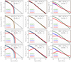 |
Fig. 2. Selection of IGIMF models representing the overall characterization of the IGIMF grid published at the CDS with this work. The metallicity used in this figure is [Fe/H] = 1, 0, −3, −5 from top to bottom; the SFR = 10−5, 100, 104 M⊙ yr−1 from left to right. All IMF models are normalized to the total stellar mass formed over δt = 10 Myr to make the comparison with the canonical IMF (black dashed line in each panel) quantitative. To compare the slope variations we plot the Salpeter-Massey slope, α = 2.3, as a grey-line grid in each plot. |
All the scripts used here are uploaded to the galIMF scripts4 such that the galIMF module can be self-consistently implemented into any chemical evolution code.
A compact quantification of the changing shape of the IGIMF for different assumptions can be achieved by calculating the mass ratios in multiple stellar mass bins. To see how relevant low-mass stars are to the total mass budget formed in δt = 10 Myr, the F05 parameter (Weidner et al. 2013a) is defined as
 (12)
(12)
This quantifies the fraction of stellar mass in stars less massive than 0.5 M⊙ relative to the total initial stellar mass. The dependency of F05 on the SFR and metallicity is shown in Fig. 4 for the different IGIMF formulations. Values F05 > 0.25 indicate bottom-heavy IGIMFs. Values of F05 > 0.6 are required to match IMF-sensitive spectral features in elliptical galaxies (La Barbera et al. 2013; Ferreras et al. 2015). Such large F05 values would not lead to very high dynamical mass-to-light ratios as the resulting IGIMF is not significantly steeper than the canonical IMF for m < 0.5 M⊙. This is very important because an IGIMF with a single Salpeter power-law index over all stellar masses would lead to unrealistically high dynamical mass-to-light ratios (see Ferreras et al. 2013).
Similarly, the mass fraction of stars with m < 0.4 M⊙ relative to the present-day stellar mass (in all stars less massive than 0.8 M⊙) is defined as
 (13)
(13)
This constitutes an approximation to a stellar population that is about 12 Gyr old. This parameter, plotted in Fig. 5, informs the bottom heaviness of the present-day stellar population ignoring stellar remnants. Furthermore, the parameter
 (14)
(14)
is the mass fraction of stars more massive than 8.0 M⊙ relative to the total initial stellar mass formed in 10 Myr, Mtot and indicates the degree of top heaviness of the IGIMFs (Fig. 6).
4.2. Evolution of gwIMF of an elliptical galaxy and its chemical evolution
The presented IGIMF grid, or the script using galIMF to produce the grid, can be readily implemented into galaxy chemical evolutionary codes to obtain a self-consistent gwIMF evolution with time. To show that the IGIMF approach is promising in this regard, we created a burst star formation history (SFH) that approximately resembles the formation of an elliptical galaxy with a total mass in all stars formed of 1012 M⊙. Its present-day roughly 12 Gyr old counterpart would according to the present results (Fig. 4) have a mass of about 2 × 10¹¹ M⊙ in main-sequence stars. The [Fe/H] enrichment, a prescribed function of time used in this work solely for the purpose of demonstration, is shown in the top panel in Fig. 3. For each δt = 10 Myr epoch the IGIMF is computed for the given SFR and [Fe/H] value. The bottom set of panels show the evolution of the IGIMF. In this example, the gwIMF is top heavy at high SFR and becomes bottom heavy during the metal-rich phase of the evolution. That is, the stellar population, as described by this IGIMF, can produce rapid α element enrichment in a fast first phase and can also potentially produce an overabundance of low-mass stars mainly in the most metal-rich centre. This is because it is plausible that star formation may continue near the centre in the high-density metal-enriched gas, which has the shortest cooling time in this region.
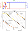 |
Fig. 3. Example of IGIMF evolution with time, plotting only the IGIMF3 model. Top panel: prescribed evolution of the SFR with time (red solid curve, left y-axis), that is the SFH, stellar mass build-up with time (blue solid curve, right y-axis) , and the metallicity evolution (upper x-axis). This example serves to show a typical evolution and therefore the curves were synthetically created. This example of how a 1012 M⊙ elliptical galaxy assembles over about 1 Gyr is consistent with downsizing (Recchi et al. 2009), but due to stellar evolution the stellar mass of this galaxy is 2 × 10¹¹ M⊙ after 12 Gyr. Using the IGIMF grid, the same principle can be applied self-consistently in a chemo-dynamical code. In addition the four vertical lines represent the chosen time snapshots shown in the bottom panels. Bottom panels: four IGIMF plots at the chosen times (see top panel), showing how the IGIMF can potentially evolve throughout elliptical galaxy assembly. Shown is the top-heavy phase, but also the bottom-heavy phase during the metal-rich part of the evolution. |
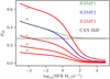 |
Fig. 4. Mass fraction formed in δt = 10 Myr in stars less massive than 0.5 M⊙ relative to the total initial mass in the IGIMF models (Eq. (12)) is shown in dependence of the SFR and [Fe/H]. The canonical IMF is depicted as the horizontal black line (F05 ≈ 0.25). We note that the IGIMF1 and IGIMF2 models lead to F05 values as if the gwIMF were bottom heavy in comparison with the canonical IMF. However this is due to the normalization caused by the IGIMF being top light for low SFRs (<1 M⊙ yr−1). |
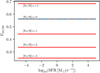 |
Fig. 5. Mass fraction formed in δt = 10 Myr in stars less massive than 0.4 M⊙ relative to the total present-day stellar mass formed in δt = 10 Myr in the IGIMF models (Eq. (13)) shown in dependence of the SFR and [Fe/H]. The canonical IMF is depicted as the horizontal black line (F04/08 ≈ 0.7), as are the IGIMF1 and IGIMF2 models as these are metallicity independent. The present-day stellar population is assumed to contain only stars less massive than 0.8 M⊙, ignoring remnant masses. The fractions are constant because these IGIMF models do not depend on the SFR for stars with m < 1 M⊙. |
 |
Fig. 6. Mass fraction formed in δt = 10 Myr in stars more massive than 8.0 M⊙ relative to the total initial mass in the IGIMF models (Eq. (14)) shown in dependence of the SFR and [Fe/H]. The canonical IMF is depicted as the horizontal black line (F80 ≈ 0.22). |
The IGIMF grid is now ready to be implemented into various chemo-dynamical codes to be tested against data in a self-consistent way.
4.3. Correction to SFR–Hα relation
Given the gwIMF varies with the SFR and metallicity of a galaxy, it is expected that any observational tracer of this SFR needs to take this into account. In the following we distinguish between the true physical SFR of a galaxy (i.e. the actual mass per unit time that is being converted to stars) versus the observationally derived SFR (e.g. SFRK in Eq. (15) below); the derived SFR requires a tracer such as the Hα flux that is often used to measure the SFR subject to an assumption concerning the shape of the gwIMF. This measure works in principle by counting the number of photons emitted from recombining hydrogen atoms such that each recombination accounts for an ionizing event, thereby the Hα flux is a measure of the flux of ionizing photons. We obtain a measure of the number of massive stars that have formed by measuring the Hα flux. We can calculate the total amount of mass converted to stars by assuming an IMF.
A widely used relationship between the galaxy-wide SFR and the measured integrated Hα flux of a galaxy is given by (Kennicutt 1998, his Eq. (2)),
 (15)
(15)
which is derived based on a single power-law IMF having a Salpeter slope (Salpeter 1955) in the mass range (0.1, 100) M⊙ assuming solar metallicity. Therefore this relation needs to be corrected for any IMF variation and metallicity, as has already been done previously (e.g. Lee et al. 2002, 2009; Pflamm-Altenburg et al. 2007).
For low SFR ≲ 1 M⊙ yr−1 and under the assumption that the universal IMF is a probability density distribution function (the Kennicutt SFRK–Hα relation; Eq. (15)), we note that large fluctuations in the measured SFRs would be obtained when applied to star-forming systems constrained by an ECMF with Mmin < mmax. The average SFR would also be biased to smaller values because the galaxy would typically lack massive stars. Such a bias can be larger than 0.5 dex for log10(SFR/(M⊙ yr−1)) ≲ −4, assuming Mmin = 20 M⊙ owing to the combination of stochastic effects and the ECMF constraint (e.g. da Silva et al. 2014). The Appendix A contains a brief comparison between the IGIMF theory and the SLUG da Silva et al. (2014) approach.
In this work corrections of the SFR–Hα function are presented in the full IGIMF (IGIMF1 and IGIMF3) framework for the first time. We note that the IGIMF2 model yields the same results as the IGMF3 model for solar metallicity and that the IGIMF1 model is metallicity independent. But a metallicity dependence enters into all IGIMF models due to the metallicity dependency of stellar evolution. For this purpose the galIMF module is linked with the PEGASE stellar population synthesis code (Fioc et al. 2011, see also Fioc & Rocca-Volmerange 1999 for an astro-ph documented manual) taking advantage of the PyPegase python wrapper5. The Hα flux is computed by PEGASE directly from the ionizing photons. Even though it is possible to introduce, for example, dust as an absorber, we do not use any additional parameters in our computations. The PEGASE code is structured such that it does not allow the input IMF or gwIMF to vary during the computation. In our application the gwIMF however varies with the SFR. Thus we limited our simulations to those with a constant SFR and metallicity over the timescale δt = 10 Myr. The gwIMF computed by the IGIMF theory is a continuous function that is approximated by multi-slope power-law functions, which are translated to an input file for PEGASE. In practice, we use four slopes to describe the calculated IGIMF: i.e. a power-law fit to each of the four mass ranges 0.08–0.5 M⊙, 0.5–1.0 M⊙, 1–0.8 mmax M⊙, 0.8 mmax–150 M⊙. This four-segment power-law description provides an excellent approximation to the full IGIMF over all stellar masses. Nevertheless, it would be better if the full numerical form of the IGIMF can be used for such calculations with PEGASE in the future; PEGASE does not currently enable an IMF to be read in as a data file but requires the IMF to be defined as power-law sections.
This allows us to calculate the Hα flux as an output from the PEGASE code for a chosen gwIMF and metallicity and thus to quantify the SFR–Hα relations for the metallicity dependent formulation of the IGIMF. From this the correction for each metallicity with respect to the Kennicut SFRK–Hα relation can be computed.
The solar-metallicity SFR–Hα relations are shown in the left panel of Fig. 7, and the sub-solar metallicity case is shown in the right panel. In addition to the Kennicutt SFRK–Hα relation and the IGIMF1,3 relations, we show the empirical correction of this relation proposed by Lee et al. (2009) based on far ultraviolet (FUV) non-ionizing continuum and Hα nebular emission, which deviates from the Kennicutt SFRK–Hα relation and is closer to the IGIMF relation.
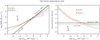 |
Fig. 7. Left panel: SFR–Hα relation. The IGIMF version in comparison with the empirical power laws proposed by Kennicutt (1998) and Lee et al. (2009). The red and green solid lines are IGIMF1/3 computed for solar metallicity [Fe/H] = 0 and the dashed lines represent the case of sub-solar metallicity, [Fe/H] = −2. Right panel: corrections to the Kennicutt SFRK–Hα relation (Eq. (17)). The true (IGIMF) SFRs are divided by the Kennicutt value. The Hα flux of LeoP is shown by the vertical dotted line in both panels. For example, from the left panel it is evident that the IGIMF1,3 models yield values of the SFR that are consistent with the presence of massive stars in the Leo P galaxy. The two panels show that dwarf galaxies with Hα fluxes near 1036 erg s−1 have a SFR that is more than 100 times larger than that suggested by the Kennicutt relation (Eq. (15)), while massive or profusely star-forming galaxies with Hα ≈ 1044 erg s−1 have SFRs that can be 10–100 times smaller than given by the traditional Kennicutt relation. As for the left panel the solid lines indicate solar metallicity [Fe/H] = 0 and the dashed lines indicate [Fe/H] = −2. |
For the purpose of general use of the corrected relations in Fig. 7, the IGIMF SFR–Hα relations are represented with third order polynomials,
 (16)
(16)
where i = 1, 3 and x = log10(LHα ergs s−1)). The polynomial coefficients for different metallicities and for the IGIMF1,3 models are summarized in Table 4. The sub-solar values are consistent with the results of Boquien et al. (2014).
The correction factor (Fig. 7) is calculated as follows:
 (17)
(17)
4.3.1. The case of the Leo P galaxy
Leo P is a late-type dwarf galaxy approximately at a distance of 1.6 Mpc, which has a metallicity [Fe/H] ≈ −1.8 and an Hα flux, LHα = 5.5 ⋅ 1036 ergs s−1. This flux comes from one HII region powered by one or two stars with individual masses of m ≈ 25 M⊙ (e.g. McQuinn et al. 2015).
We use the measured Hα flux as a star formation indicator with the newly developed SFR indicators of Sect. 4.3. Table 5 summarizes the computed SFRs based on different assumptions. The masses of the most massive star and second-most massive star are calculated for the IGIMF1 and IGIMF3 models (IGIMF2 is indistinguishable from IGIMF3; see also Yan et al. 2017) using the values of the SFR derived from the observed Hα luminosity. The most massive star has a mass of 23–26 M⊙, the second most massive star has a mass in the range 16–20 M⊙. That is, according to the IGIMF theory, the SFRIGIMF, i of Leo P would be significantly larger than the standard value, SFRK(LHα), being consistent with the presence of the observed massive stars in Leo P. The SLUG approach (see Appendix A) also implies a larger true SFR than given by the standard value (Fig. 3 in da Silva et al. 2014).
SFR of Leo P based on the observed Hα flux.
The message to be taken away from this discussion is that when the Hα flux is used as a star-formation indicator to test the IGIMF theory the appropriate Hα SFR relation also needs to be employed. Pflamm-Altenburg et al. (2007) already emphasized that there is a physical limit to the SFR if a galaxy forms a single star only at a given time (their Eq. (16)); these authors also pointed out that distant late-type dwarf galaxies are likely to have Hα-dark star formation. In the limit where only few ionizing stars form, the UV-flux derived SFRs are more robust and these are indeed consistent with the higher SFRs as calculated using the IGIMF1 formulation. This is shown explicitly in Fig. 8 of Lee et al. (2009), who compared UV- and Hα-based SFR indicators for dwarf galaxies for which the original IGIMF formulations (IGIMF1, which did not include the IMF variation of Marks et al. 2012) remain valid. We add a note of caution that part of the discrepancies between the Hα– and UV-based SFR indicators may be influenced by several physical effects, such as the different gas phases (such as the diffuse inoized gas present in galaxies), photon leakage from HII regions, gas, and dust abundance. Calzetti et al. (2013) and also for example Kennicutt & Evans (2012) provide a more detailed discussion of various SFR tracers and their interrelations.
McQuinn et al. (2015) constructed the optical colour-magnitude diagram (CMD) for Leo P in order to infer its SFH and assumed the invariant canonical IMF for this purpose, i.e. the authors assumed the caninvgwIMF hypothesis of Table 1. An issue worthy of future study is to quantify the degeneracies between the shape of the gwIMF and the derived SFH. Unfortunately, the implementation of a variable gwIMF into the time-dependent scheme that would allow the self-consistent modelling of the SFH while reproducing the full CMD has not been done for the IGIMF theory yet. Knowing the SFRIGIMF,i within the IGIMF theory using the Hα flux allows us to discuss possible effects in the CMD and the whole low-mass stellar population in the galaxy, as is touched upon in the next section.
4.3.2. Implications for the BTFR and the CMD
Given the higher SFRs in the IGIMF theory produced by the top-light gwIMF, the positions of Leo P and other dwarf galaxies in the BTFR (McGaugh et al. 2000; Lelli et al. 2016) need be considered as a consistency check. That is, if there is substantial dark star formation it might alter the total mass of the galaxy, assuming an age.
This problem is relevant also for the dark matter problem and notably for Milgromian gravitation (MOND; Milgrom 1983; Famaey & McGaugh 2012). The application of the IGIMF theory to dwarf galaxies has already shown (Pflamm-Altenburg & Kroupa 2009) that the build-up times of the observed stellar populations (as assessed using the luminosity) is well accounted for within less than a Hubble time (see their Figs. 10 and 11), solving the problem according to which such galaxies need longer than a Hubble time to form their stellar content if the SFR was not significantly larger in the past. Applying the IGIMF theory to dwarf galaxies therefore does not change their baryonic masses, it merely shortens their gas-consumption timescale (Pflamm-Altenburg & Kroupa 2009) and allows them to form stellar populations within a Hubble time. The BTFR therefore remains untouched.
For the case of Leo P, the known extent and baryonic matter in Leo P and the flat (non-rising) part of the rotational curve are prone to uncertainty and therefore more observational data are required (Giovanelli et al. 2013) to constrain the position of Leo P in the BTFR.
Another consistency test is to study if the observed CMD of Leo P can be reproduced within the IGIMF theory. This needs further work and it is to be noted that the central stellar population is similar to a canonical stellar population; for example, in the IGIMF theory the central embedded cluster that formed the two 25 M⊙ stars is, by construction, canonical for solar metallicity. A detailed calculation and comparison with the observed CMD needs to resort to the local IGIMF formulation (Sect. 5.1) that allows the spacial integration of stellar populations within a galaxy (Pflamm-Altenburg & Kroupa 2008).
4.4. Ultra-faint dwarf galaxies
Recent measurements with the Hubble Space Telescope by Gennaro et al. (2018b) of UFD satellite galaxies, as an extension of the study by Geha et al. (2013), have suggested a possible gwIMF variation in these galaxies in the stellar-mass range (0.4–0.8 M⊙). The authors, however, mentioned that a larger data sample is needed to improve the reliability of the presented results. In this work we use the gwIMF variations derived by Gennaro et al. (2018b) as an illustrative case to show how the gwIMF variations can constrain the stellar IMF on star cluster scales using the IGIMF approach. But in order to draw more robust conclusions and firmer constraints on the low-mass end of the IMF slopes (α1, α2) further measurements in such objects are required.
Figure 8 shows inferred and measured values by Gennaro et al. (2018b) in comparison with the canonical IMF and IGIMF formulations as defined in Sect. 3.3. Gennaro et al. (2018b) assumed that the gwIMF can be reprsented by a single power-law form to derive the slope of the gwIMF in the mass range 0.4–0.8 M⊙. To be able to compare these measurements with the two-part power law in the IGIMF parametrization, we compute the single power-law fit to the IGIMF/canonical IMF in the same mass range. We can see that the IGIMF predictions do not describe the Gennaro et al. (2018b) data well although the general trend is reproduced. The local IMF variations used in this work to calculate the IGIMF models are based on an extrapolation from data values in the range [Fe/H] ∈ (−0.5,0) (Kroupa 2001; Marks et al. 2012). Based on this new observation of the gwIMF in the low-mass regime at metallicities in the range [Fe/H] ∈ (−3, −2), a refinement of Eq. (10) may be needed, i.e.
![Mathematical equation: $ \begin{equation} \alpha_{1,2}^{\mathrm{cor}} = \alpha_{1\mathrm{c},2\mathrm{c}} + \Delta \alpha^{\mathrm{cor}} \left(\mathrm{[Fe/H]+2.3}\right), \label{eq:alphaSPSUNDSCRcor} \end{equation} $](/articles/aa/full_html/2018/12/aa33055-18/aa33055-18-eq23.gif) (18)
(18)
where Δαcor ≈ 2.5. For [Fe/H] > −2.3 the canonical IMF would be valid in this formulation. It may be possible to identify a systematic variation of the local IMF for low-mass stars with additional data that cover a larger metallicity range and test the robustness of these results given the uncertainties. Any such new constraints must, however, be consistent with the observationally derived stellar mass functions in present-day GCs.
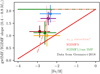 |
Fig. 8. Variable gwIMF in the stellar mass regime (0.4–0.8 M⊙) for 6 UFDs shown by the coloured points from Gennaro et al. (2018b). The IGIMF1 models (given by two slopes α1 = 1.3 and α2 = 2.3) are represented by the horizontal green line. These have the same effective invariant slope as the canonical IMF in this mass regime. The IGIMF3 metallicity-dependent effective slope based on Eq. (10) is shown in red. These data may indicate the necessity for a different dependency of the α1,2 indices on metallicity than represented by Eq. (10). This different dependency is indicated by the orange dot-dashed line (Eq. (18)). |
As a caveat we note that additional factors affect the empirically determined present-day mass function power-law index in UFDs. For example, the fraction of unresolved multiple systems may be different in the dwarfs as it depends on the dynamical history of the population (Marks & Kroupa 2012; Marks et al. 2012). Also, the final deduced index may be affected by the formation of the stellar population in embedded clusters that expel their residual gas, leading to expanding low-mass stellar populations that may be lost from a weak UFD potential. This process is exaggerated if the embedded clusters formed mass segregated (Haghi et al. 2015). In addition to this the gwIMF slopes of Gennaro et al. (2018b) are sensitive to the mass of the lowest stellar mass that is measured and to the form of the gwIMF that is assumed. In Gennaro et al. (2018a), these authors used a two-part power-law gwIMF for the case of the Coma Berenices UFD finding a smaller variation with respect to the MW.
5. Discussion
5.1. Local or regional cIMF
The gwIMF variation is parametrized within the IGIMF framework with global galaxy properties, namely the total SFR and the average metallicity. As an output we obtain the total stellar population formed in 10 Myr without any information about its spatial distribution in a galaxy. In reality, however, the gas density and metallicity varies spatially and therefore a mathematical formulation of the cIMF (Table 1), which takes into account the local gas surface density and metallicity at some position within the galaxy, is needed. A cIGIMF version has been formulated by (Pflamm-Altenburg & Kroupa 2008, the “local” IGIMF). These authors applied the IGIMF1 formulation and assumed the disc galaxy to be subdivided into radial annular bins within each of which the local IGIMF is calculated subject to the constraint that the galaxy has an exponential radial structure and the gas and SFR densities are related. This work showed that the radial Hα cut-off and extended UV discs can be explained naturally within the IGIMF framework because in the outskirts the gas density is low. This leads to a low SFR density, low-mass embedded clusters, and thus a deficit of ionizing stars, while intermediate-mass stars form there. In addition, the cIGIMF results in metallicity gradients, as are suggested to be present for example in elliptical galaxies (McConnell et al. 2016), and provides a description for low surface-brightness galaxies (LSBGs) having low gas surface densities (Pflamm-Altenburg et al. 2011). Based on the cIGIMF calculation, LSBGs form preferentially low-mass stars with a deficit of high-mass stars relative to the canonical IMF even though the global SFR can be high and the IGIMF would predict that massive stars will be formed. We plan to include a mathematically and physically consistent cIGIMF description in the next version of the galIMF code originally developed by Yan et al. (2017).
5.2. Changes to IMF variations within IGIMF framework
As formulated in this work, the IGIMF implements several empirical relations such as the star-mass function of embedded clusters, its variation, the correlation between the birth radius and mass of the embedded clusters, and local IMF variations with the physical conditions in the star-forming cloud core. Since these are empirically derived not covering all possible physical values (extreme SFRs and metallicities are not accessible in the Local Universe for example), the IGIMF prescription applied in this work can be improved with time. That is, obtaining better data or data from environments not yet probed on a galactic scale and on larger scales can be used to infer local IMF variations. This has been shown in this paper for the case of UFD measurements from Gennaro et al. (2018b; see Fig. 8 and Eq. (18)) in contrast to the original empirical extrapolation from MW data described by Eq. (10).
Any proposed changes can be readily implemented into the galIMF code (Yan et al. 2017) and further tested. However any local IMF variations need to match the canonical IMF for a SFR comparable to that of the MW and an average MW metallicity as well as the present-day mass functions observed in globular clusters, open clusters, and embedded clusters as a necessary constraint on any viable IMF theory.
6. Conclusions
For the first time a grid of gwIMFs computed within the IGIMF framework with SFR and metallicity dependence is presented, together with its implementation into the galIMF module and an equivalent FORTRAN code. This allow us to trace the variations of gwIMFs for different galaxies assuming that the physics driving the gwIMFs comes from local star-forming regions. The main contributions of this work can be summarized as follows:
– The attached IGIMF grid with the parameter-span SFR ∈(10−5, 104) and [Fe/H] ∈(−5, 1) presents the gwIMF normalized to the total stellar mass formed in 10 Myr episodes, Mtot = SFR × 10 Myr; the individual stars always have the same range of masses (from 0.08 to 120 M⊙) for an implementation into galaxy-evolution (e.g. chemo-dynamical evolution) codes and also for a possible interpolation in the grid.
– The overall variation of the gwIMF is as follows: (1) The gwIMF can become top light even if the shape of the local stellar IMF is invariant (IGIMF1 version). This can been explained with a demonstrative example: 1000 star clusters with a mass of 10 M⊙ would have a top-light stellar population in comparison to a monolithically formed star cluster of 104 M⊙ because stars more massive than 10 M⊙ would exist only in the latter case (Yan et al. 2017). This statement is basically independent of metallicity and reflects the fact that there is a maximum stellar mass that forms in a given cluster because of the mmax = WK(Mecl) relation. Also the upper limit for the most massive star cluster to be formed in a galaxy depends on galactic properties (Johnson et al. 2017). The top-light IGIMF appears to be in good agreement with gwIMF measurements in nearby dwarf galaxies (Lee et al. 2009; Watts et al. 2018). The above demonstrative example is actually found in nature (Hsu et al. 2012, 2013). (2) The gwIMF, as expected, is close to the canonical IMF for a SFR near 1M⊙ yr−1 and solar metallicity and becomes top heavy with increasing SFR above that value. (3) Interestingly, for sub-solar metallicity the gwIMF can be bottom light and for super-solar metallicity bottom heavy (according to the IGIMF3 parametrization which includes the full metallicity and density variation of the stellar IMF). This might be reflected in the cores of elliptical galaxies.
– We present the possible time evolution of the gwIMF for the case of a monolithic (star-burst) formation of an elliptical galaxy showing the potential to explain observed features: high α element abundances implying a short formation timescale, high metallicity implying a top-heavy gwIMF during this short assembly time, and an overabundance of low-mass stars indicating a metal-rich formation epoch in which the gwIMF is bottom heavy.
– As a consequence of the variable gwIMF the majority of standard and widely used stellar-population correlations used to estimate galaxy properties need to be recomputed and re-interpreted correctly. This is because assumptions concerning the IMF enter into many of these correlations. This is shown using the SFR–Hα relation. Assuming the IGIMF theory to be the correct description it follows that the SFR is underestimated for galaxies with a low SFR and it is overestimated for galaxies with high SFRs, by up to several orders of magnitude, if the standard Kennicutt SFRK–Hα relation is used. We present the appropriate correction factors (Fig. 7). The Leo P galaxy, often mentioned as posing a significant problem for the IGIMF theory because for the estimated SFR stars as massive as 25 M⊙ should not be forming in this galaxy, is shown to be well reproduced using the IGIMF theory. This is because in the literature the Kennicutt SFRK–Hα relation is incorrectly applied when star cluster masses are smaller than the most massive stars, i.e. when Mmin < mmax. In this case the ensemble of freshly formed star clusters contain low-mass clusters within which the IMF cannot be sampled to the most massive stars in the case of the IMF being a constrained probability distribution as in the SLUG approach (Appendix A). This implies a systematic deficit of massive stars in the whole ensemble. This produces a biased result when the Kennicutt relation is extrapolated to low Hα fluxes, that is when SFRK ≲ 10−4 M⊙ yr−1 because the Kennicutt relation assumes all star formation events to always have a fully sampled IMF (da Silva et al. 2012). This is naturally corrected for in the IGIMF theory such that the observed galaxy (e.g. Leo P) behaves physically correctly (see Fig. 7).
– The data by Gennaro et al. (2018b) for UFD galaxies have suggested a possible variation of the low-mass IMF for stars in the mass range (0.4–0.8 M⊙) and metallicity in the range ([Fe/H] = −3 to −2). The IMF variations over this mass range and metallicity range have not been constrained empirically and only an extrapolation has been applied in this work (Kroupa 2001; Marks et al. 2012, see Eq. (10)). The IGIMF theory is used to translate the observed galaxy-wide variation to a possible variation of the IMF and therewith to possibly improve the formulation of the local IMF variation in this stellar mass range and at low metallicity ([Fe/H] = −3 to −2). The newly suggested variation (see Eq. (18) and Fig. 8) shows how gwIMF measurements can help constrain star formation on star cluster scales, but we note the caveats discussed in Sect. 4.4.
The IGIMF theory which is, by construction, consistent with MW data, has now demonstrated its general potential in allowing the computations of gwIMFs from local empirical stellar IMF properties; this theory also has the ability to improve our understanding of how the IMF varies in embedded clusters. It is ready to be implemented into chemo-dynamical codes and to be tested with more data. First implementations of the IGIMF theory into self-consistent galaxy formation and evolution simulations have been achieved (Bekki 2013; Ploeckinger et al. 2014). The implications of the IGIMF theory for the gas-depletion and stellar-mass build-up timescales of galaxies are significant (Pflamm-Altenburg & Kroupa 2009); many other galaxy-evolution problems are potentially resolved naturally (Pflamm-Altenburg et al. 2011). The SFR correction factors shown in Fig. 7 need to be applied to the traditional Kennicutt values and, in general, entail significantly larger true SFRs for low-mass, star-dominated populations in dwarf galaxies with a general shift to significantly smaller true SFRs for massive star-forming galaxies. These correction factors (Eq. (17)) lead to a change of the slope of the galaxy main sequence (Speagle et al. 2014), which will be addressed in an upcoming contribution. Finally, the occurrence of Hα-dark star formation may significantly affect the cosmological SFR (Pflamm-Altenburg et al. 2007).
We note that we use “local” to mean a small region in a galaxy and in this case an embedded-cluster-forming molecular cloud core. It is not the solar neighbourhood.
The Nbody star cluster evolution computations available on youtube, “Dynamical ejection of massive stars from a young star cluster” by Seungkyung Oh based on Oh et al. (2015), Oh & Kroupa (2016), demonstrate how dynamically active the binary-rich very young clusters are in dispersing their stars to relatively large distances.
Acknowledgments
The authors acknowledge the exceptionally useful and comprehensive comments from an anonymous referee. We also thank to ESO visitor programme for supporting AV and PK during their stay. We thank Frederico Lelli for useful discussions and comments to the manuscript. AV {acknowledges} support from grant AYA2016-77237-C3-1-P from the Spanish Ministry of Economy and Competitiveness (MINECO). AHZ acknowledges support from Alexander von Humboldt Foundation through a Research Fellowship. The discussions and the provided references by Neal Evans are also acknowledged.
References
- Adams, F. C., & Fatuzzo, M. 1996, ApJ, 464, 256 [NASA ADS] [CrossRef] [Google Scholar]
- André, P., Revéret, V., Könyves, V., et al. 2016, A&A, 592, A54 [NASA ADS] [CrossRef] [EDP Sciences] [Google Scholar]
- Ascenso, J. 2018, in The Birth of Star Clusters, ed. S. Stahler, Astrophys. Space Sci. Libr., 424, 1 [NASA ADS] [CrossRef] [Google Scholar]
- Ballesteros-Paredes, J., Klessen, R. S., Mac Low, M. M., & Vazquez-Semadeni, E. 2007, Protostars and Planets V, 63 [Google Scholar]
- Banerjee, S., & Kroupa, P. 2013, ApJ, 764, 29 [NASA ADS] [CrossRef] [Google Scholar]
- Banerjee, S., & Kroupa, P. 2014, ApJ, 787, 158 [NASA ADS] [CrossRef] [Google Scholar]
- Banerjee, S., & Kroupa, P. 2015, MNRAS, 447, 728 [NASA ADS] [CrossRef] [Google Scholar]
- Banerjee, S., & Kroupa, P. 2017, A&A, 597, A28 [NASA ADS] [CrossRef] [EDP Sciences] [Google Scholar]
- Banerjee, S., Kroupa, P., & Oh, S. 2012, MNRAS, 426, 1416 [NASA ADS] [CrossRef] [Google Scholar]
- Bastian, N., Covey, K. R., & Meyer, M. R. 2010, ARA&A, 48, 339 [NASA ADS] [CrossRef] [Google Scholar]
- Bate, M. R., Tricco, T. S., & Price, D. J. 2014, MNRAS, 437, 77 [NASA ADS] [CrossRef] [Google Scholar]
- Baumgardt, H., & Makino, J. 2003, MNRAS, 340, 227 [NASA ADS] [CrossRef] [Google Scholar]
- Bekki, K. 2013, MNRAS, 436, 2254 [NASA ADS] [CrossRef] [Google Scholar]
- Binney, J., & Tremaine, S. 1987, Galactic Dynamics (Princeton, NJ: Princeton University Press), 747 [Google Scholar]
- Boquien, M., Buat, V., & Perret, V. 2014, A&A, 571, A72 [NASA ADS] [CrossRef] [EDP Sciences] [Google Scholar]
- Bressert, E., Bastian, N., Gutermuth, R., et al. 2010, MNRAS, 409, L54 [NASA ADS] [Google Scholar]
- Brinkmann, N., Banerjee, S., Motwani, B., & Kroupa, P. 2017, A&A, 600, A49 [NASA ADS] [CrossRef] [EDP Sciences] [Google Scholar]
- Calzetti, D. 2013, in Star Formation Rate Indicators, eds. J. Falcón-Barroso, & J. H. Knapen, 419 [Google Scholar]
- Chabrier, G. 2003, PASP, 115, 763 [NASA ADS] [CrossRef] [Google Scholar]
- Conroy, C., van Dokkum, P. G., & Villaume, A. 2017, ApJ, 837, 166 [NASA ADS] [CrossRef] [Google Scholar]
- da Silva, R. L., Fumagalli, M., & Krumholz, M. 2012, ApJ, 745, 145 [NASA ADS] [CrossRef] [Google Scholar]
- da Silva, R. L., Fumagalli, M., & Krumholz, M. R. 2014, MNRAS, 444, 3275 [NASA ADS] [CrossRef] [Google Scholar]
- Dabringhausen, J., Kroupa, P., & Baumgardt, H. 2009, MNRAS, 394, 1529 [NASA ADS] [CrossRef] [Google Scholar]
- Dabringhausen, J., Fellhauer, M., & Kroupa, P. 2010, MNRAS, 403, 1054 [Google Scholar]
- Dabringhausen, J., Kroupa, P., Pflamm-Altenburg, J., & Mieske, S. 2012, ApJ, 747, 72 [NASA ADS] [CrossRef] [Google Scholar]
- De Masi, C., Matteucci, F., & Vincenzo, F. 2018, MNRAS, 474, 5259 [NASA ADS] [CrossRef] [Google Scholar]
- Dobbs, C. L., Burkert, A., & Pringle, J. E. 2011, MNRAS, 413, 2935 [NASA ADS] [CrossRef] [Google Scholar]
- Duarte-Cabral, A., Bontemps, S., Motte, F., et al. 2013, A&A, 558, A125 [NASA ADS] [CrossRef] [EDP Sciences] [Google Scholar]
- Egusa, F., Kohno, K., Sofue, Y., Nakanishi, H., & Komugi, S. 2009, ApJ, 697, 1870 [NASA ADS] [CrossRef] [Google Scholar]
- Egusa, F., Sofue, Y., & Nakanishi, H. 2004, PASJ, 56, L45 [NASA ADS] [Google Scholar]
- Elmegreen, B. G. 2002, ApJ, 577, 206 [NASA ADS] [CrossRef] [Google Scholar]
- Elmegreen, B. G. 2007, ApJ, 668, 1064 [NASA ADS] [CrossRef] [Google Scholar]
- Famaey, B., & McGaugh, S. S. 2012, Living Rev. Relativ., 15, 10 [Google Scholar]
- Federrath, C. 2015, MNRAS, 450, 4035 [NASA ADS] [CrossRef] [Google Scholar]
- Federrath, C. 2016, MNRAS, 457, 375 [NASA ADS] [CrossRef] [Google Scholar]
- Federrath, C., Schrön, M., Banerjee, R., & Klessen, R. S. 2014, ApJ, 790, 128 [NASA ADS] [CrossRef] [Google Scholar]
- Ferreras, I., La Barbera, F., de la Rosa, I. G., et al. 2013, MNRAS, 429, L15 [NASA ADS] [CrossRef] [Google Scholar]
- Ferreras, I., Weidner, C., Vazdekis, A., & La Barbera, F. 2015, MNRAS, 448, L82 [NASA ADS] [CrossRef] [Google Scholar]
- Figer, D. F. 2005, Nature, 434, 192 [NASA ADS] [CrossRef] [PubMed] [Google Scholar]
- Fioc, M., & Rocca-Volmerange, B. 1999, ArXiv e-prints [arXiv:astro-ph/9912179] [Google Scholar]
- Fioc, M., Le Borgne, D., & Rocca-Volmerange, B. 2011, Astrophysics Source Code Library [record ascl:1108.007] [Google Scholar]
- Fontanot, F., De Lucia, G., Hirschmann, et al. 2017, MNRAS, 464, 3812 [NASA ADS] [CrossRef] [Google Scholar]
- Fontanot, F., De Lucia, G., Xie, L., et al. 2018a, MNRAS, 475, 2467 [NASA ADS] [Google Scholar]
- Fontanot, F., La Barbera, F., De Lucia, G., Pasquali, A., & Vazdekis, A. 2018b, MNRAS, 479, 5678 [NASA ADS] [CrossRef] [Google Scholar]
- Fukui, Y., & Kawamura, A. 2010, ARA&A, 48, 547 [NASA ADS] [CrossRef] [Google Scholar]
- Geha, M., Brown, T. M., Tumlinson, J., et al. 2013, ApJ, 771, 29 [NASA ADS] [CrossRef] [Google Scholar]
- Gennaro, M., Geha, M., Tchernyshyov, K., et al. 2018a, ApJ, 863, 38 [NASA ADS] [CrossRef] [Google Scholar]
- Gennaro, M., Tchernyshyov, K., Brown, T. M., et al. 2018b, ApJ, 855, 20 [NASA ADS] [CrossRef] [Google Scholar]
- Gieles, M., Moeckel, N., & Clarke, C. J. 2012, MNRAS, 426, L11 [NASA ADS] [CrossRef] [Google Scholar]
- Giovanelli, R., Haynes, M. P., Adams, E. A. K., et al. 2013, AJ, 146, 15 [NASA ADS] [CrossRef] [Google Scholar]
- Gunawardhana, M. L. P., Hopkins, A. M., Sharp, R. G., Brough, S., et al. 2011, MNRAS, 415, 1647 [NASA ADS] [CrossRef] [Google Scholar]
- Hacar, A., Alves, J., Tafalla, M., & Goicoechea, J. R. 2017a, A&A, 602, L2 [NASA ADS] [CrossRef] [EDP Sciences] [Google Scholar]
- Hacar, A., Tafalla, M., & Alves, J. 2017b, A&A, 606, A123 [NASA ADS] [CrossRef] [EDP Sciences] [Google Scholar]
- Haghi, H., Zonoozi, A. H., Kroupa, P., Banerjee, S., & Baumgardt, H. 2015, MNRAS, 454, 3872 [NASA ADS] [CrossRef] [Google Scholar]
- Haghi, H., Khalaj, P., Hasani Zonoozi, A., & Kroupa, P. 2017, ApJ, 839, 60 [NASA ADS] [CrossRef] [Google Scholar]
- Hansen, C. E., Klein, R. I., McKee, C. F., & Fisher, R. T. 2012, ApJ, 747, 22 [NASA ADS] [CrossRef] [Google Scholar]
- Hartmann, L., Ballesteros-Paredes, J., & Bergin, E. A. 2001, ApJ, 562, 852 [NASA ADS] [CrossRef] [Google Scholar]
- Hasani Zonoozi, A., Mahani, H., & Kroupa, P. 2018, MNRAS, accepted [ arXiv:1810.00034] [Google Scholar]
- Heggie, D., & Hut, P. 2003, The Gravitational Million-Body Problem: A Multidisciplinary Approach to Star Cluster Dynamics (Cambridge: Cambridge University Press) [CrossRef] [Google Scholar]
- Hopkins, A. M. 2018, PASA, accepted [arXiv:1807.09949] [Google Scholar]
- Hsu, W.-H., Hartmann, L., Allen, L., et al. 2012, ApJ, 752, 59 [NASA ADS] [CrossRef] [Google Scholar]
- Hsu, W.-H., Hartmann, L., Allen, L., et al. 2013, ApJ, 764, 114 [NASA ADS] [CrossRef] [Google Scholar]
- Jeřábková, T., Kroupa, P., Dabringhausen, J., Hilker, M., & Bekki, K. 2017, A&A, 608, A53 [NASA ADS] [CrossRef] [EDP Sciences] [Google Scholar]
- Johnson, L. C., Seth, A. C., Dalcanton, J. J., et al. 2017, ApJ, 839, 78 [NASA ADS] [CrossRef] [Google Scholar]
- Joncour, I., Duchêne, G., Moraux, E., & Motte, F. 2018, A&A, in press, DOI: 10.1051/0004-6361/201833042 [Google Scholar]
- Kalari, V. M., Carraro, G., Evans, C. J., & Rubio, M. 2018, ApJ, 857, 132 [NASA ADS] [CrossRef] [Google Scholar]
- Kennicutt, R. C. J. 1998, ARA&A, 36, 189 [Google Scholar]
- Kennicutt, R. C., & Evans, N. J. 2012, ARA&A, 50, 531 [NASA ADS] [CrossRef] [Google Scholar]
- Kirk, H., & Myers, P. C. 2011, ApJ, 727, 64 [NASA ADS] [CrossRef] [Google Scholar]
- Kirk, H., & Myers, P. C. 2012, ApJ, 745, 131 [NASA ADS] [CrossRef] [Google Scholar]
- Koen, C. 2006, MNRAS, 365, 590 [NASA ADS] [CrossRef] [Google Scholar]
- Kroupa, P. 2001, MNRAS, 322, 231 [NASA ADS] [CrossRef] [Google Scholar]
- Kroupa, P. 2002, Science, 295, 82 [NASA ADS] [CrossRef] [PubMed] [Google Scholar]
- Kroupa, P. 2005, in The Three-Dimensional Universe with Gaia, eds. C. Turon, K. S. O’Flaherty, & M. A. C. Perryman, ESA SP, 576, 629 [NASA ADS] [Google Scholar]
- Kroupa, P. 2015, Can. J. Phys., 93, 169 [NASA ADS] [CrossRef] [Google Scholar]
- Kroupa, P., & Boily, C. M. 2002, MNRAS, 336, 1188 [NASA ADS] [CrossRef] [Google Scholar]
- Kroupa, P., & Bouvier, J. 2003, MNRAS, 346, 343 [NASA ADS] [CrossRef] [Google Scholar]
- Kroupa, P., & Jerabkova, T. 2018, ArXiv e-prints [arXiv:1806.10605] [Google Scholar]
- Kroupa, P., & Weidner, C. 2003, ApJ, 598, 1076 [NASA ADS] [CrossRef] [Google Scholar]
- Kroupa, P., Tout, C. A., & Gilmore, G. 1993, MNRAS, 262, 545 [NASA ADS] [CrossRef] [Google Scholar]
- Kroupa, P., Aarseth, S., & Hurley, J. 2001, MNRAS, 321, 699 [NASA ADS] [CrossRef] [Google Scholar]
- Kroupa, P., Weidner, C., Pflamm-Altenburg, J., et al. 2013, The Stellar and Sub-Stellar Initial Mass Function of Simple and Composite Populations (Berlin: Springer), 115 [Google Scholar]
- Kroupa, P., Jeˇrábková, T., Dinnbier, F., Beccari, G., & Yan, Z. 2018, A&A, 612, A74 [NASA ADS] [CrossRef] [EDP Sciences] [Google Scholar]
- La Barbera, F., Ferreras, I., Vazdekis, A., et al. 2013, MNRAS, 433, 3017 [NASA ADS] [CrossRef] [Google Scholar]
- Lada, C. J. 2010, Trans. R. Soc. London Ser. A, 368, 713 [Google Scholar]
- Lada, C. J., & Lada, E. A. 2003, ARA&A, 41, 57 [NASA ADS] [CrossRef] [Google Scholar]
- Lee, J. C., Salzer, J. J., Impey, C., Thuan, T. X., & Gronwall, C. 2002, AJ, 124, 3088 [NASA ADS] [CrossRef] [Google Scholar]
- Lee, J. C., Gil de Paz, A., Tremonti, C., et al. 2009, ApJ, 706, 599 [NASA ADS] [CrossRef] [Google Scholar]
- Leisawitz, D. 1989, BAAS, 21, 1189 [NASA ADS] [Google Scholar]
- Lelli, F., McGaugh, S. S., & Schombert, J. M. 2016, ApJ, 816, L14 [Google Scholar]
- Lieberz, P., & Kroupa, P. 2017, MNRAS, 465, 3775 [NASA ADS] [CrossRef] [Google Scholar]
- Lim, B., Sung, H., Bessell, M. S., et al. 2018, MNRAS, 477, 1993 [NASA ADS] [CrossRef] [Google Scholar]
- Lu, X., Zhang, Q., Liu, H. B., et al. 2018, ApJ, 855, 9 [NASA ADS] [CrossRef] [Google Scholar]
- Lucas, W. E., Rybak, M., Bonnell, I. A., & Gieles, M. 2018, MNRAS, 474, 3582 [Google Scholar]
- Machida, M. N., & Matsumoto, T. 2012, MNRAS, 421, 588 [NASA ADS] [Google Scholar]
- Maíz Apellániz, J.,Walborn, N. R., Morrell, N. I., Niemela, V. S., & Nelan, E. P. 2007, ApJ, 660, 1480 [NASA ADS] [CrossRef] [Google Scholar]
- Marks, M., & Kroupa, P. 2012, A&A, 543, A8 [NASA ADS] [CrossRef] [EDP Sciences] [Google Scholar]
- Marks, M., Kroupa, P., Dabringhausen, J., & Pawlowski, M. S. 2012, MNRAS, 422, 2246 [NASA ADS] [CrossRef] [Google Scholar]
- Marks, M., Kroupa, P., Dabringhausen, J., & Pawlowski, M. S. 2014, MNRAS, 442, 3315 [NASA ADS] [CrossRef] [Google Scholar]
- Martín-Navarro, I. 2016, MNRAS, 456, L104 [NASA ADS] [CrossRef] [Google Scholar]
- Massey, P. 2003, ARA&A, 41, 15 [NASA ADS] [CrossRef] [Google Scholar]
- Matteucci, F. 1994, A&A, 288, 57 [NASA ADS] [Google Scholar]
- McConnell, N. J., Lu, J. R., & Mann, A. W. 2016, ApJ, 821, 39 [NASA ADS] [CrossRef] [Google Scholar]
- McGaugh, S. S., Schombert, J. M., Bothun, G. D., & de Blok, W. J. G. 2000, ApJ, 533, L99 [NASA ADS] [CrossRef] [PubMed] [Google Scholar]
- McQuinn, K. B. W., Skillman, E. D., Dolphin, A., et al. 2015, ApJ, 812, 158 [NASA ADS] [CrossRef] [Google Scholar]
- Megeath, S. T., Gutermuth, R., Muzerolle, J., et al. 2016, AJ, 151, 5 [NASA ADS] [CrossRef] [Google Scholar]
- Meidt, S. E., Hughes, A., Dobbs, C. L., et al. 2015, ApJ, 806, 72 [NASA ADS] [CrossRef] [Google Scholar]
- Meurer, G. R., Wong, O. I., Kim, J. H., et al. 2009, ApJ, 695, 765 [NASA ADS] [CrossRef] [Google Scholar]
- Milgrom, M. 1983, ApJ, 270, 365 [NASA ADS] [CrossRef] [Google Scholar]
- Mor, R., Robin, A. C., Figueras, F., & Lemasle, B. 2017, A&A, 599, A17 [NASA ADS] [CrossRef] [EDP Sciences] [Google Scholar]
- Mor, R., Robin, A. C., Figueras, F., & Antoja, T. 2018, A&A, in press, DOI: 10.1051/0004-6361/201833501 [Google Scholar]
- Neuhäuser, R., Frink, S., Röser, S. R., et al. 1998, Acta Hist. Astron., 3, 206 [NASA ADS] [Google Scholar]
- Oey, M. S., & Clarke, C. J. 2005, ApJ, 620, L43 [NASA ADS] [CrossRef] [Google Scholar]
- Offner, S. S. R., Clark, P. C., Hennebelle, P., et al. 2014, Protostars and Planets VI, 53 [Google Scholar]
- Oh, S., & Kroupa, P. 2012, MNRAS, 424, 65 [NASA ADS] [CrossRef] [Google Scholar]
- Oh, S., & Kroupa, P. 2016, A&A, 590, A107 [NASA ADS] [CrossRef] [EDP Sciences] [Google Scholar]
- Oh, S., Kroupa, P., & Pflamm-Altenburg, J. 2015, ApJ, 805, 92 [NASA ADS] [CrossRef] [Google Scholar]
- Padoan, P., Pan, L., Haugbølle, T., & Nordlund, Å. 2016, ApJ, 822, 11 [NASA ADS] [CrossRef] [Google Scholar]
- Padoan, P., Haugbølle, T., Nordlund, Å., & Frimann, S. 2017, ApJ, 840, 48 [NASA ADS] [CrossRef] [Google Scholar]
- Papadopoulos, P. P. 2010, ApJ, 720, 226 [NASA ADS] [CrossRef] [Google Scholar]
- Pflamm-Altenburg, J., & Kroupa, P. 2008, Nature, 455, 641 [NASA ADS] [CrossRef] [PubMed] [Google Scholar]
- Pflamm-Altenburg, J., & Kroupa, P. 2009, ApJ, 706, 516 [NASA ADS] [CrossRef] [Google Scholar]
- Pflamm-Altenburg, J., Weidner, C., & Kroupa, P. 2007, ApJ, 671, 1550 [NASA ADS] [CrossRef] [Google Scholar]
- Pflamm-Altenburg, J., Weidner, C., & Kroupa, P. 2009, MNRAS, 395, 394 [NASA ADS] [CrossRef] [Google Scholar]
- Pflamm-Altenburg, J., Weidner, C., & Kroupa, P. 2011, in UP2010: Have Observations Revealed a Variable Upper End of the Initial Mass Function? eds. M. Treyer, T. Wyder, J. Neill, M. Seibert, & J. Lee, ASP Conf. Ser., 440, 269 [NASA ADS] [Google Scholar]
- Pflamm-Altenburg, J., González-Lópezlira, R. A., & Kroupa, P. 2013, MNRAS, 435, 2604 [NASA ADS] [CrossRef] [Google Scholar]
- Ploeckinger, S., Hensler, G., Recchi, S., Mitchell, N., & Kroupa, P. 2014, MNRAS, 437, 3980 [NASA ADS] [CrossRef] [Google Scholar]
- Plunkett, A. L., Fernández-López, M., Arce, H. G., et al. 2018, A&A, 615, A9 [NASA ADS] [CrossRef] [EDP Sciences] [Google Scholar]
- Qiu, K., Zhang, Q., Beuther, H., & Yang, J. 2007, ApJ, 654, 361 [NASA ADS] [CrossRef] [Google Scholar]
- Qiu, K., Zhang, Q., Megeath, S. T., et al. 2008, ApJ, 685, 1005 [NASA ADS] [CrossRef] [Google Scholar]
- Qiu, K., Zhang, Q., & Menten, K. M. 2011, ApJ, 728, 6 [NASA ADS] [CrossRef] [Google Scholar]
- Ramírez Alegría, S., Borissova, J., Chené, A.-N., et al. 2016, A&A, 588, A40 [NASA ADS] [CrossRef] [EDP Sciences] [Google Scholar]
- Recchi, S., & Kroupa, P. 2015, MNRAS, 446, 4168 [NASA ADS] [CrossRef] [Google Scholar]
- Recchi, S., Calura, F., & Kroupa, P. 2009, A&A, 499, 711 [NASA ADS] [CrossRef] [EDP Sciences] [Google Scholar]
- Renaud, F., Famaey, B., & Kroupa, P. 2016, MNRAS, 463, 3637 [NASA ADS] [CrossRef] [Google Scholar]
- Romano, D., Matteucci, F., Zhang, Z.-Y., Papadopoulos, P. P., & Ivison, R. J. 2017, MNRAS, 470, 401 [NASA ADS] [CrossRef] [Google Scholar]
- Salpeter, E. E. 1955, ApJ, 121, 161 [Google Scholar]
- Scalo, J. M. 1986, Fund. Cosmic Phys., 11, 1 [NASA ADS] [EDP Sciences] [Google Scholar]
- Schneider, F. R. N., Sana, H., Evans, C. J., et al. 2018, Science, 359, 69 [NASA ADS] [CrossRef] [Google Scholar]
- Schulz, C., Pflamm-Altenburg, J., & Kroupa, P. 2015, A&A, 582, A93 [NASA ADS] [CrossRef] [EDP Sciences] [Google Scholar]
- Selman, F. J., & Melnick, J. 2008, ApJ, 689, 816 [NASA ADS] [CrossRef] [Google Scholar]
- Smith, N., Stassun, K. G., & Bally, J. 2005, AJ, 129, 888 [NASA ADS] [CrossRef] [Google Scholar]
- Speagle, J. S., Steinhardt, C. L., Capak, P. L., & Silverman, J. D. 2014, ApJS, 214, 15 [NASA ADS] [CrossRef] [Google Scholar]
- Stephens, I. W., Gouliermis, D., Looney, L. W., et al. 2017, ApJ, 834, 94 [NASA ADS] [CrossRef] [Google Scholar]
- Tafalla, M., Myers, P. C., Caselli, P., Walmsley, C. M., & Comito, C. 2002, ApJ, 569, 815 [NASA ADS] [CrossRef] [Google Scholar]
- van Dokkum, P. G., & Conroy, C. 2010, Nature, 468, 940 [NASA ADS] [CrossRef] [Google Scholar]
- Vanbeveren, D. 1982, A&A, 115, 65 [NASA ADS] [Google Scholar]
- Vazdekis, A., Peletier, R. F., Beckman, J. E., & Casuso, E. 1997, ApJS, 111, 203 [NASA ADS] [CrossRef] [Google Scholar]
- Watts, A. B., Meurer, G. R., Lagos, C. D. P., et al. 2018, MNRAS, 477, 5554 [NASA ADS] [CrossRef] [Google Scholar]
- Weidner, C., & Kroupa, P. 2004, MNRAS, 348, 187 [NASA ADS] [CrossRef] [Google Scholar]
- Weidner, C., & Kroupa, P. 2005, ApJ, 625, 754 [NASA ADS] [CrossRef] [Google Scholar]
- Weidner, C., & Kroupa, P. 2006, MNRAS, 365, 1333 [NASA ADS] [CrossRef] [Google Scholar]
- Weidner, C., Kroupa, P., & Larsen, S. S. 2004, MNRAS, 350, 1503 [NASA ADS] [CrossRef] [Google Scholar]
- Weidner, C., Kroupa, P., & Bonnell, I. A. D. 2010, MNRAS, 401, 275 [NASA ADS] [CrossRef] [Google Scholar]
- Weidner, C., Ferreras, I., Vazdekis, A., & La Barbera, F. 2013a, MNRAS, 435, 2274 [NASA ADS] [CrossRef] [Google Scholar]
- Weidner, C., Kroupa, P., Pflamm-Altenburg, J., & Vazdekis, A. 2013b, MNRAS, 436, 3309 [NASA ADS] [CrossRef] [Google Scholar]
- Weidner, C., Kroupa, P., & Pflamm-Altenburg, J. 2013c, MNRAS, 434, 84 [NASA ADS] [CrossRef] [Google Scholar]
- Whitmore, B. C., Zhang, Q., Leitherer, C., et al. 1999, AJ, 118, 1551 [NASA ADS] [CrossRef] [Google Scholar]
- Wright, N. J., & Mamajek, E. E. 2018, MNRAS, 476, 381 [NASA ADS] [CrossRef] [Google Scholar]
- Wu, J., Evans, II., N. J., Shirley, Y. L., & Knez, C. 2010, ApJS, 188, 313 [NASA ADS] [CrossRef] [Google Scholar]
- Wuchterl, G., & Tscharnuter, W. M. 2003, A&A, 398, 1081 [NASA ADS] [CrossRef] [EDP Sciences] [Google Scholar]
- Yan, Z., Jerabkova, T., & Kroupa, P. 2017, A&A, 607, A126 [NASA ADS] [CrossRef] [EDP Sciences] [Google Scholar]
- Zhang, Q., Fall, S. M., & Whitmore, B. C. 2001, ApJ, 561, 727 [NASA ADS] [CrossRef] [Google Scholar]
- Zonoozi, A. H., Haghi, H., & Kroupa, P. 2016, ApJ, 826, 89 [NASA ADS] [CrossRef] [Google Scholar]
- Zhang, Z.-Y., Romano, D., Ivison, R. J., Papadopoulos, P. P., & Matteucci, F. 2018, Nature, 558, 260 [NASA ADS] [CrossRef] [Google Scholar]
Appendix A: The stochastically lighting up galaxies
The stochastically lighting up galaxies (SLUG) approach (da Silva et al. 2014) is an alternative to the newer IGIMF formulation; this alternative approach implements star formation basically using principles from a first formulation of the IGIMF theory (Kroupa & Weidner 2003; Weidner & Kroupa 2005, 2006). In SLUG, a galaxy is constructed by first drawing the masses of star clusters. These star clusters are then filled up with stars by randomly choosing from an IMF until the cluster mass is reached (da Silva et al. 2014, their Sect. 2.1). Therefore this is not fully random sampling but mass-constrained sampling instead (Weidner & Kroupa 2006). This means that it is impossible to have a 100 M⊙ star in a 80 M⊙ star cluster, for example. The SLUG approach therefore is along the original IGIMF approach, which fundamentally rests on the notion that the stellar population in a galaxy is formed in star clusters and thus constitutes conditional stochasticity (Kroupa & Weidner 2003; Weidner & Kroupa 2006). We note however that the SLUG approach differs from the current IGIMF formulations by not explicitly accounting for the mmax–Mecl relation since each cluster is assumed to be populated randomly by stars subject to the mass constraint.; the published IGIMF work fulfils this constraint. Whether there is a physical function mmax = WK(Mecl) is thus an important problem to continue to study. The SLUG approach therefore does not comprise pure stochastic sampling from a gwIMF, which would yield no deficit in ionizing stars on average for galaxies with low SFRs (Pflamm-Altenburg et al. 2009). Instead, in SLUG (as in a original form of the IGIMF theory), a deficit comes about because of the mass constraint on the stars within a cluster imposed by the masses of the star clusters. The SLUG approach is thus a useful tool for comparison with the IGIMF theory as applied in this work; the IGIMF method is deterministic because it is related to the concept that star formation is strongly feedback self-regulated, by imposing the additional condition (in addition to the cluster mass Mecl) that the mmax–Mecl relation be obeyed. We also note that similar ideas to those underlying the IGIMF theory have been considered by Vanbeveren (1982).
All Tables
All Figures
|
Fig. 1. Schematic showing a late-type galaxy. Its field population is represented by red and orange stars. The newly formed stellar population is indicated by coloured circles that represent CSFEs (embedded star clusters). The colours and sizes of symbols scale with stellar/cluster mass. The acronyms from Table 3 are shown here with examples. Right bottom panel: a young massive embedded cluster, which will most likely survive and contribute to the open star cluster population of the galaxy. Right top panel: young embedded cluster complex composed of a number of low-mass embedded clusters, which will evolve into a T Tauri association once the embedded clusters expand after loss of their residual gas and disperse into the galaxy field stellar population. |
| In the text | |
|
Fig. 2. Selection of IGIMF models representing the overall characterization of the IGIMF grid published at the CDS with this work. The metallicity used in this figure is [Fe/H] = 1, 0, −3, −5 from top to bottom; the SFR = 10−5, 100, 104 M⊙ yr−1 from left to right. All IMF models are normalized to the total stellar mass formed over δt = 10 Myr to make the comparison with the canonical IMF (black dashed line in each panel) quantitative. To compare the slope variations we plot the Salpeter-Massey slope, α = 2.3, as a grey-line grid in each plot. |
| In the text | |
|
Fig. 3. Example of IGIMF evolution with time, plotting only the IGIMF3 model. Top panel: prescribed evolution of the SFR with time (red solid curve, left y-axis), that is the SFH, stellar mass build-up with time (blue solid curve, right y-axis) , and the metallicity evolution (upper x-axis). This example serves to show a typical evolution and therefore the curves were synthetically created. This example of how a 1012 M⊙ elliptical galaxy assembles over about 1 Gyr is consistent with downsizing (Recchi et al. 2009), but due to stellar evolution the stellar mass of this galaxy is 2 × 10¹¹ M⊙ after 12 Gyr. Using the IGIMF grid, the same principle can be applied self-consistently in a chemo-dynamical code. In addition the four vertical lines represent the chosen time snapshots shown in the bottom panels. Bottom panels: four IGIMF plots at the chosen times (see top panel), showing how the IGIMF can potentially evolve throughout elliptical galaxy assembly. Shown is the top-heavy phase, but also the bottom-heavy phase during the metal-rich part of the evolution. |
| In the text | |
|
Fig. 4. Mass fraction formed in δt = 10 Myr in stars less massive than 0.5 M⊙ relative to the total initial mass in the IGIMF models (Eq. (12)) is shown in dependence of the SFR and [Fe/H]. The canonical IMF is depicted as the horizontal black line (F05 ≈ 0.25). We note that the IGIMF1 and IGIMF2 models lead to F05 values as if the gwIMF were bottom heavy in comparison with the canonical IMF. However this is due to the normalization caused by the IGIMF being top light for low SFRs (<1 M⊙ yr−1). |
| In the text | |
|
Fig. 5. Mass fraction formed in δt = 10 Myr in stars less massive than 0.4 M⊙ relative to the total present-day stellar mass formed in δt = 10 Myr in the IGIMF models (Eq. (13)) shown in dependence of the SFR and [Fe/H]. The canonical IMF is depicted as the horizontal black line (F04/08 ≈ 0.7), as are the IGIMF1 and IGIMF2 models as these are metallicity independent. The present-day stellar population is assumed to contain only stars less massive than 0.8 M⊙, ignoring remnant masses. The fractions are constant because these IGIMF models do not depend on the SFR for stars with m < 1 M⊙. |
| In the text | |
|
Fig. 6. Mass fraction formed in δt = 10 Myr in stars more massive than 8.0 M⊙ relative to the total initial mass in the IGIMF models (Eq. (14)) shown in dependence of the SFR and [Fe/H]. The canonical IMF is depicted as the horizontal black line (F80 ≈ 0.22). |
| In the text | |
|
Fig. 7. Left panel: SFR–Hα relation. The IGIMF version in comparison with the empirical power laws proposed by Kennicutt (1998) and Lee et al. (2009). The red and green solid lines are IGIMF1/3 computed for solar metallicity [Fe/H] = 0 and the dashed lines represent the case of sub-solar metallicity, [Fe/H] = −2. Right panel: corrections to the Kennicutt SFRK–Hα relation (Eq. (17)). The true (IGIMF) SFRs are divided by the Kennicutt value. The Hα flux of LeoP is shown by the vertical dotted line in both panels. For example, from the left panel it is evident that the IGIMF1,3 models yield values of the SFR that are consistent with the presence of massive stars in the Leo P galaxy. The two panels show that dwarf galaxies with Hα fluxes near 1036 erg s−1 have a SFR that is more than 100 times larger than that suggested by the Kennicutt relation (Eq. (15)), while massive or profusely star-forming galaxies with Hα ≈ 1044 erg s−1 have SFRs that can be 10–100 times smaller than given by the traditional Kennicutt relation. As for the left panel the solid lines indicate solar metallicity [Fe/H] = 0 and the dashed lines indicate [Fe/H] = −2. |
| In the text | |
|
Fig. 8. Variable gwIMF in the stellar mass regime (0.4–0.8 M⊙) for 6 UFDs shown by the coloured points from Gennaro et al. (2018b). The IGIMF1 models (given by two slopes α1 = 1.3 and α2 = 2.3) are represented by the horizontal green line. These have the same effective invariant slope as the canonical IMF in this mass regime. The IGIMF3 metallicity-dependent effective slope based on Eq. (10) is shown in red. These data may indicate the necessity for a different dependency of the α1,2 indices on metallicity than represented by Eq. (10). This different dependency is indicated by the orange dot-dashed line (Eq. (18)). |
| In the text | |
Current usage metrics show cumulative count of Article Views (full-text article views including HTML views, PDF and ePub downloads, according to the available data) and Abstracts Views on Vision4Press platform.
Data correspond to usage on the plateform after 2015. The current usage metrics is available 48-96 hours after online publication and is updated daily on week days.
Initial download of the metrics may take a while.