| Issue |
A&A
Volume 620, December 2018
The XXL Survey: second series
|
|
|---|---|---|
| Article Number | A8 | |
| Number of page(s) | 13 | |
| Section | Cosmology (including clusters of galaxies) | |
| DOI | https://doi.org/10.1051/0004-6361/201731321 | |
| Published online | 20 November 2018 | |
The XXL Survey
XXIII. The mass scale of XXL clusters from ensemble spectroscopy★
1
Department of Physics and Michigan Center for Theoretical Physics, University of Michigan,
Ann Arbor,
MI 48109, USA
e-mail: aryaf@umich.edu
2
INAF–Osservatorio astronomico di Padova,
Vicolo Osservatorio 5,
35122 Padova, Italy
3
Aix Marseille Univ., CNRS, CNES, LAM, Marseille, France
4
Department of Physics and Astronomy, University of Padova,
Vicolo Osservatorio 3,
35122 Padova, Italy
5
Department of Astronomy, University of Michigan,
Ann Arbor,
MI 48109, USA
6
INAF–Osservatorio Astronomico di Bologna,
via Ranzani 1,
40127 Bologna, Italy
7
Istituto di Astrofisica Spaziale e Fisica Cosmica Milano,
via Bassini 15,
20133 Milan, Italy
8
School of Physics,
HH Wills Physics Laboratory,
Tyndall Avenue,
Bristol, BS8 1TL, UK
9
Center for Astrophysics and Space Astronomy, Department of Astrophysical and Planetary Science, University of Colorado,
Boulder,
CO 80309, USA
10
NASA Ames Research Center,
Moffett Field,
CA 94035, USA
11
Dipartimento di Fisica e Astronomia, Università di Bologna,
viale Berti Pichat 6/2,
40127 Bologna, Italy
12
Herschel Science Centre, European Space Astronomy Centre, ESA, 28691 Villanueva de la Cañada, Spain
13
Astrophysics Research Institute, Liverpool John Moores University, IC2, Liverpool Science Park,
146 Brownlow Hill, Liverpool L3 5RF, UK
14
INAF–Osservatorio Astronomico di Roma,
via Frascati 33, 00078 Monte Porzio Catone (Rome), Italy
15
School of Physics, Monash University,
Clayton,
Victoria 3800, Australia
16
International Centre for Radio Astronomy Research (ICRAR), The University of Western Australia, M468,
35 Stirling Highway, Crawley, WA 6009, Australia
17
SUPA, School of Physics and Astronomy, University of St Andrews,
North Haugh, St Andrews KY16 9SS, UK
18
Main Astronomical Observatory, Academy of Sciences of Ukraine,
27 Akademika Zabolotnoho St.,
03680 Kyiv, Ukraine
19
Astrophysics and Cosmology Research Unit, University of KwaZulu-Natal,
4041 Durban, South Africa
20
Australian Astronomical Observatory,
Box 915, North Ryde 1670, Australia
21
INAF,
Osservatorio Astronomico di Brera,
via Brera 28,
20159 Milano, Italy
22
AIM, CEA, CNRS, Univ. Paris-Saclay, Univ. Paris Diderot,
Sorbonne Paris Cité,
91191 Gif-sur-Yvette, France
23
Universität Hamburg,
Hamburger Sternwarte,
Gojenbergsweg 112,
21029 Hamburg, Germany
24
Laboratoire Lagrange, UMR 7293, Université de Nice Sophia Antipolis, CNRS, Observatoire de la Côte d'Azur,
06304 Nice, France
25
Department of Physics and Astronomy, Macquarie University,
NSW 2109,
Australia and Australian Astronomical Observatory PO Box 915, North Ryde NSW 1670, Australia
26
Argelander Institut für Astronomie,
Universität Bonn,
Auf dem Huegel 71,
53121 Bonn, Germany
27
Aristotle University of Thessaloniki, Physics Department,
54124 Thessaloniki, Greece
28
Instituto Nacional de Astrofísica Óptica y Electrónica,
AP 51 y 216,
72000 Puebla, Mexico
29
IAASARS, National Observatory of Athens,
15236 Penteli, Greece
30
School of Physics and Astronomy, University of Birmingham, Edgbaston, Birmingham B15 2TT, UK
31
Ulugh Beg Astronomical Institute of Uzbekistan Academy of Science,
33 Astronomicheskaya str.,
Tashkent,
100052 Uzbekistan
32
Max-Planck Institut füer Kernphysik,
Saupfercheckweg 1,
69117 Heidelberg, Germany
Received:
6
June
2017
Accepted:
14
November
2017
Context. An X-ray survey with the XMM-Newton telescope, XMM-XXL, has identified hundreds of galaxy groups and clusters in two 25 deg2 fields. Combining spectroscopic and X-ray observations in one field, we determine how the kinetic energy of galaxies scales with hot gas temperature and also, by imposing prior constraints on the relative energies of galaxies and dark matter, infer a power-law scaling of total mass with temperature.
Aims. Our goals are: i) to determine parameters of the scaling between galaxy velocity dispersion and X-ray temperature, T300 kpc, for the halos hosting XXL-selected clusters, and; ii) to infer the log-mean scaling of total halo mass with temperature, ⟨lnM200 | T300 kpc, z⟩.
Methods. We applied an ensemble velocity likelihood to a sample of >1500 spectroscopic redshifts within 132 spectroscopically confirmed clusters with redshifts z < 0.6 to model, ⟨lnσgal | T300 kpc, z⟩, where σgal is the velocity dispersion of XXL cluster member galaxies and T300 kpc is a 300 kpc aperture temperature. To infer total halo mass we used a precise virial relation for massive halos calibrated by N-body simulations along with a single degree of freedom summarising galaxy velocity bias with respect to dark matter.
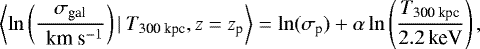
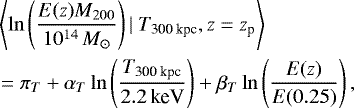
Results. For the XXL-N cluster sample, we find σgal ∝ T300 kpc0.63±0.05, a slope significantly steeper than the self-similar expectation of 0.5. Assuming scale-independent galaxy velocity bias, we infer a mean logarithmic mass at a given X-ray temperature and redshift, 〈ln(E(z)M200/1014 M⊙)|T300 kpc, z〉 = πT + αT ln (T300 kpc/Tp) + βT ln (E(z)/E(zp)) using pivot values kTp = 2.2 keV and zp = 0.25, with normalization πT = 0.45 ± 0.24 and slope αT = 1.89 ± 0.15. We obtain only weak constraints on redshift evolution, βT = −1.29 ± 1.14.
Conclusions. The ratio of specific energies in hot gas and galaxies is scale dependent. Ensemble spectroscopic analysis is a viable method to infer mean scaling relations, particularly for the numerous low mass systems with small numbers of spectroscopic members per system. Galaxy velocity bias is the dominant systematic uncertainty in dynamical mass estimates.
Key words: galaxies: clusters: general / X-rays: galaxies: clusters / galaxies: kinematics and dynamics / galaxies: groups: general
© ESO 2018
1 Introduction
The cosmic web of dark matter drives the gravitational potential wells in which baryonic matter is accelerated, shocked, stirred, and partially cooled into stars and galaxies. Under gravity and shocks alone, the internal structure of collapsed halos is anticipated to be self-similar (Bertschinger 1985), meaning that the internal density and temperature profiles for hot gas maintain fixed forms in an appropriately scaled spatial radius. Integration of these forms enables straightforward calculation of global properties such as X-ray luminosity or temperature. The model specifies the slopes and evolution with redshift of key mass-observable relations (MORs, see Kaiser 1986).
While astrophysical processes within halos, such as star formation and associated supernova and active galactic nuclei (AGN) feedback, are expected to drive deviations from self-similarity, the observed population mean behaviour of the most massive halos lie close to self-similar predictions (Mantz et al. 2016a).
The idea that both galaxies and hot gas are in virial equilibrium within a common gravitational potential, originally proposed by Cavaliere & Fusco-Femiano (1976), leads to the expectation that galaxy velocity dispersion scales as the square root of X-ray temperature,  . This behaviour reflects MOR scalings with total mass
  and
and  at fixed redshift.
For the most massive clusters in the sky, multiple surveys and follow-up observations are enabling individual halo masses to be estimated from gravitational lensing, hydrostatic, and dynamical methods (see Allen et al. 2011; Kravtsov & Borgani 2012, for reviews). These methods are subject to different sources of systematic uncertainty (e.g., Meneghetti et al. 2014), and the samples to which they are applied may have additional systematic shifts, relative to a sample complete in halo mass, due to sample selection. The resulting biases pose limits on the accuracy of empirically derived MORs.
Multiple, independent mass proxies allow for consistency tests that can expose and help mitigate systematic errors. We present here a virial analysis of 132 spectroscopically confirmed clusters identified in the XMM-XXL Survey (Pierre et al. 2016, hereafter XXL Paper I). The method extends the stacked spectroscopic technique developed by Farahi et al. (2016), originally applied to optically selected clusters in SDSS (Rykoff et al. 2014).
We focus first on the virial scaling of galaxy velocity dispersion with hot gas temperature, then infer how mean total mass scales with temperature using an additional degree of freedom that relates galaxy velocity dispersion to the underlying dark matter. This galaxy velocity bias is the largest source of uncertainty in our mass estimate.
Early N-body simulations established virial scaling for purely dark matter halos (Evrard 1989) and ensemble analysis of billion-particle and larger simulations provides a highly accurate calibration, with sub-percent error in the intercept of dark matter velocity dispersion at fixed halo mass (Evrard et al. 2008).
Inferring a virial, or dynamical, mass of an individual cluster requires a large number of spectroscopic members and a reliable interloper rejection algorithm (e.g., Biviano et al. 2006) such as that provided by the caustic technique (Rines et al. 2007; Rines & Diaferio 2010; Gifford et al. 2013). For large cluster samples emerging from surveys, a complementary approach to infer mean MOR scaling behaviour is to employ ensemble population analysis, effectively stacking the local velocities of galaxies in multiple clusters to extract a mean velocity dispersion signal (Farahi et al. 2016).
Here we have employed a large collection of galaxy spectroscopic redshifts assembled from multiple sources for groups and clusters identified in the north field of the XMM-XXL survey. The 132 systems span X-ray temperatures kT300 kpc ∈ [0.48−6.03] keV, and redshift z ∈ [0.03−0.6], and the spectroscopic sources include GAMA, SDSS-DR10, VIPERS, and VVDS Deep and Ultra Deep surveys.
The mass-temperature scaling has been studied extensively (e.g., Xue & Wu 2000; Ortiz-Gil et al. 2004; Arnaud et al. 2005; Vikhlinin et al. 2006; Kettula et al. 2015; Mantz et al. 2016b; Lieu et al. 2016). Observational relations generally steepen from close to the self-similar for hot systems to a slope of ~ 1.6−1.7 once cooler systems (kT300 kpc ≲ 3 keV) are included(Arnaud et al. 2005; Lieu et al. 2016). More than half of the clusters in this work will be systems with kT300 kpc ≲ 3 keV, which allows us to test deviation from the self-similar model, with yet another mass calibration technique.
As part of the first series of XXL papers, (Lieu et al. 2016, hereafter XXL Paper IV) estimates the mass-temperature scaling relation of X-ray bright systems using weak-lensing mass measurements from the Canada-France-Hawaii Telescope Lensing Survey (CFHTLenS) shear catalogueue (Heymans et al. 2012; Erben et al. 2013). The work presented here is complementary to that study where it provides a mean dynamical mass as a function of X-ray temperature. The X-ray sample differs from that used by XXL Paper IV, but the pipeline for deriving X-ray properties from the XMM data is identical.
We describe the sample, data, and selection criteria in Sect. 2. The likelihood model used to constrain the galaxy velocity dispersion scaling with temperature is described in Sect. 3. In Sect. 4, we present results for this relation, followed by a discussion of a range of systematic uncertainties and sensitivity analysis in Sect. 5. A key result of this work, the dynamical mass-temperature relation, is presented in Sect. 6. Finally we conclude in Sect. 7
Throughout we have assumed WMAP9 consistent cosmology with Ωm = 0.28, ΩDE = 0.72, and local Hubble constant h = H0∕100 km s−1 Mpc−1 = 0.7. Unless otherwise noted, our convention for the mass of a halo is M200, the mass contained within a spherical region encompassing a mean density equal to 200 times the critical density of the Universe, ρc(z). Similarly, rΔ is defined as the radius of the sphere inside which the mean density is a factor Δ times the critical density of the Universe at that redshift, and MΔ is the total mass within that radius.
2 Cluster and spectroscopic sample
The XXL survey consists of tiled 10 ks (or longer) exposures across two fields of roughly 25 deg2 each. The observing strategy and science goals of the survey are described in XXL Paper I while source selection and a resultant brightest 100 cluster sample are published in Pacaud et al. (2016, hereafter XXL Paper II). The X-ray images were processed with the XAMIN v3.3.2 pipeline (Pacaud et al. 2006), which produces lists of detections of varying quality. The overall catalogue with point sources will be available in computer readable form via the XXL Master Catalogue browser1 and at the Centre de Données astronomiques de Strasbourg (CDS2; Chiappetti et al. 2018, hereafter XXL Paper XXVIII), while cluster candidates are grouped by detection classes (C1, C2, C3) and hosted in the same places as catalogue XXL-365-GC (Adami et al. 2018, hereafter XXL Paper XX). The 2016 series of XXL papers, including (XXL Paper II), pertained to the brightest 100 clusters and 1000 AGN, while for the second series, including this paper, we are publishing much deeper samples: 365 clusters and 20 000 AGN, with slightly revised cluster properties and scaling relations. Of the XXL cluster sample 46% are classified as high-quality (C1) detections, 43% are intermediate quality (C2) and the remaining 11% are marginal quality (C3) sources. We discard C3 sources in this work as they do not have reliable luminosity and temperature measurements. The subject of this work is a subset in the XXL-N area, with spectroscopically confirmed redshifts and with redshifts z < 0.6, generating asample of 132 systems. A detailed discussion of the sample selection is provided by XXL Paper XX and Guglielmo et al. (2018, hereafter XXL Paper XXII). The cluster optical and X-ray images can be found in the XXL cluster database3.
The skydistribution of the systems used in this work is shown in Fig. 1. X-ray extended sources are shown as black circlesand the colour map shows the sky surface density of spectroscopic galaxies lying in an aperture of radius r ≤ 3r500 with respect to their centres. The r500 estimates are determined from weak lensing mass estimates presented in XXL Paper IV. We next provide additional details of the group/cluster and galaxy spectroscopic samples.
2.1 X-ray Temperatures
Of the 132 spectroscopically confirmed C1 and C2 clusters with z < 0.6, X-ray temperatures are available for 106, 81 C1 and 25 C2 clusters. All are C1 clusters and most but not all are included in the XXL 100 brightest sample of XXL Paper II. The temperature determination, described in detail by Giles et al. (2016, hereafter XXL Paper III), outputs the temperature measured within a physical 300 kpc aperture for sufficiently high signal-to-noise-ratio systems.
After detection by XAMIN v3.3.2 – a detection pipeline piloted by the XMM-LSS project (Pacaud et al. 2006) – as an extended X-ray source, a background subtracted radial profile is extracted in the [0.5− 2] keV band. The detection radius is defined as that at which the source is detected at 5σ above the background. A spectrum is then fit from a circular aperture of radius of 300 kpc centred on the X-ray centroid, using a minimum of five counts per energy bin, resulting in a temperature measurement we refer to as T300 kpc. Cluster spectral fits were performed in the 0.4−7.0 keV band with an absorbed APEC model with the absorbing column fixed at the Galactic value, and a fixed metal abundance of Z = 0.3 Z⊙. For more detail on the data processing, we refer the reader to Pacaud et al. (2016). We note that the measured X-ray temperatures are non-core excised owing to the limited angular resolution of XMM-Newton and the modest signal-to-noise-ratio of most detections. These temperatures are taken from XXL Paper XX.
For the systems that lack direct temperature estimates, we estimate temperatures from X-ray luminosities using published XXL scaling relations as follows. First, background-corrected XMM count-rates within 300 kpc from the cluster centre in the [0.5− 2] keV band are extracted. This forms the basis of a first luminosity estimate, the starting point for an iterative scheme that uses the L − T scaling relation from XXL Paper XX and the T − M500 relation from XXL Paper IV. The process assumes isothermal β-model emission with parameters (rc, β) = (0.15r500, 2∕3), and iterations continue until convergence. This method outputs temperature, mass, and r500 estimates. Details of the steps above are described and reported in XXL Paper XX.
To check the internal consistency of the derived X-ray temperature, XXL Paper XX performs a comparison of T300 kpc derived using the above approach with direct temperature measurements for a subset of systems, finding good agreement. Below, we show that the velocity dispersion scaling parameters using the subset of systems with directly measured temperatures are consistent with those of the full cluster sample.
Figure 2 shows redshifts and temperatures of the XXL-N clusters. At a given redshift, higher mass systems that are both brighter and hotter tend to have direct temperature measurements. As explained in Sect. 2.5, the sample size shrinks, by roughly 3% (four clusters), after we apply velocity and aperture cuts discussed below.
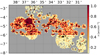 |
Fig. 1 Spatial distribution of galaxies and clusters in the XXL north field used in this work. Black circles show cluster centres with z ≤ 0.6 with area proportional to temperature. The heat map shows the sky surface density of spectroscopic galaxies lying within a projected aperture of 3r500 around cluster centres. |
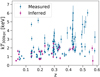 |
Fig. 2 Temperature vs. redshift of the full 132 XXL-N cluster sample. Blue circles are clusters with measured temperature and magenta squares show clusters with inferred temperature. |
2.2 Spectroscopic sample
Concerning the spectroscopic database of galaxies, reduced spectra from several public surveys are combined with XXL dedicated observing runs to create a large, heterogeneous collection of redshifts. The surveys and observing programmes, listed in Table 2 in XXL Paper XXII, include GAMA (45%; Hopkins et al. 2013; Liske et al. 2015), SDSS-DR10 (5% Ahn et al. 2014), VIPERS (32% Guzzo et al. 2014), VVDS Deep and Ultra Deep (9% Le Fèvre et al. 2005, 2015). The remaining 9% are obtained mainly by ESO Large Programme + WHT XXL dedicated observational campaigns which are individually contributing less than 2%. The typical error in redshift for galaxies is ~0.00041(1 + z), equivalent to 120(1 + z) km s^-1. The full list of spectroscopic catalogues are listed in XXL Paper XXII. We note that the spectroscopic sample adopted in this work is a subset of the spectroscopic sample of XXL Paper XXII.
Given that the catalogue sources overlap in the sky, a non-negligible number of objects are observed by more than one project. The cleaning of catalogue duplicates follows the selection criteria designed to identify the best spectrum in the final catalogue, as described by XXL Paper XXII. The selection procedure is based on two sets of priorities, the first regarding source origin and then the second regarding the reliability flag attributed to the redshift estimate.
The full sample contains 120 506 galaxies in the north XXL region, 63 681 of which are at z ≤ 0.6. For our default analysis, we employ a sub-sample comprised of those galaxies lying within a projected distance of r500 from the centres of the clusters, shown in Fig. 1, yielding 7751 galaxies.
The spectroscopic information for these galaxies, as well as for spectroscopically confirmed groups/clusters, is hosted in the CeSAM (Centre de donnéeS Astrophysiques de Marseille) database in Marseille (CeSAM-DR2)4.
2.3 Spectroscopic redshifts of XXL-selected clusters
All C1 and C2 candidate clusters identified within the XXL survey are followed up for spectroscopic redshifts using an iterative semi-automatic process similar to that used for the XMM-LSS survey (Adami et al. 2011).
First, spectroscopic redshifts from public and private sources lying within the X-ray contours are selected. These are sorted to identify significant (more than 3 galaxies) concentrations, including a preliminary “cluster population” based on projected separation from the X-ray centroid. For the large majority of cases, a single concentration appears, allowing for relatively unambiguous redshift determination.
A preliminary measure of the cluster redshift is the mean value of the redshift of the preliminary cluster population. From this redshift, a physical region of 500 kpc radius is defined, and all galaxies within this radius were selected as cluster members. This procedure is iterated with all available redshifts within a 500 kpc physical radius to get the final mean cluster redshift. However, for ambiguous cases where there are not more than three galaxies with spectroscopic redshifts, the redshift is measured by looking for the putative brightest cluster galaxy (BCG) in the i-band located close to the X-ray centroid (see XXL Paper XX for a detailed discussion).
The cluster centre is defined by the peak in the detected X-ray emission. Because X-ray emission is continuous and the gas traces the gravitational potential, we expect fewer mis-centred clusters (mis-centered with respect to the dark matter potential minimum) compared to photometrically-defined samples (Rykoff et al. 2012). We defer a detailed treatment of cluster mis-centring to future work.
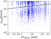 |
Fig. 3 Magnitude of the rest-frame velocity of cluster galaxies, Eq. (1), as a function of cluster temperature. Each dot is one galaxy, and some galaxies appear in the fields of multiple clusters. The black line shows the cut, Eq. (2), that separates the lower signal population from a projected background. Points above the black line are disregarded in our analysis. |
2.4 Galaxy-cluster velocities
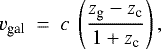
Given the redshift, zc, of each XXL-N group or cluster, we measure the rest-frame relative velocity of each galaxy within the target field of that cluster,
 (1)
(1)
where c is the speed of light and zg is the redshift of the galaxy.
In this paper the original spectroscopic galaxy selection for each cluster is defined only by sky location, not cluster redshift. Therefore, each cluster field contains a mix of galaxies residing within and outside the cluster environment. We describe below the probabilisticmethod originally applied to SDSS redMaPPer systems by Rozo et al. (2015), which involves a two-stage approach to handling foreground and background galaxies.
2.5 Signal component and final cluster sample
The model framework, wherein observable properties scale with halo mass as power laws with some intrinsic covariance, motivates the modeling process. For systems with a given temperature, T300kpc, and redshift, we expect a log-normal distribution of halo mass with some intrinsic (10− 20%) scatter (Le Brun et al. 2016). The galaxy velocities internal to these halos are assumed to follow a Gaussian distribution with a dispersion that increases with halo mass. Because the intrinsic scatter of these relations is not very large, the expected distribution of galaxy velocities, vgal, at fixed T300 kpc and z will also be close to Gaussian (see Becker et al. 2007, for a specific model applied to galaxy richness instead of temperature). This collective component is the fundamental signal we seek to model and extract from the data.
The first stage of the process removes projected interlopers with large vgal offsets, much larger than those expected from the underlying Gaussian model. The threshold value, vmax(T300 kpc), is set empirically by examination of the absolute magnitude of the line-of-sight galaxy velocities as a function of cluster temperature, given in Fig. 3. Similar to the analysis of Farahi et al. (2016), where redMaPPer optical richness plays the role of T300kpc, two populations emerge: a signal component at low velocities and a projected population offset to higher velocities.
Based on the structure of Fig. 3, we define a maximum, rest-frame galaxy velocity for the signal region of
 (2)
(2)
Applying this cut along with the radial cut, r ≤ r500, eliminates four clusters from the sample because no galaxies satisfy these cuts. The final cluster sample involves 1592 galaxies across 128 clusters, 103 of which have directly measured temperatures.
Figure 4 shows the distribution of spectroscopic galaxy counts within r500 in the cluster sample after applying the velocity threshold, Eq. (2). The modal, median, and mean values are 3, 9, and 12.4 respectively. After applying the velocity and aperture cuts, the main contribution of spectroscopic sample came from GAMA (45%), VIPERS (30%), VVDS Deep and Ultra Deep (11%), SDSS-DR10 (5%). The remaining catalogues individually contribute less than 2%.
In Sect. 5, we investigate the sensitivity of our results to vmax and r500 selection thresholds, not finding statistically significant change.
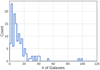 |
Fig. 4 Frequency distribution of the number of spectroscopic members per cluster within r500 after removing the high-velocity background component using the velocity cut, Eq. (2). |
3 Cluster ensemble velocity model
The study of Rozo et al. (2015) introduced an ensemble likelihood model for stacked cluster spectroscopy with the goal of assessing the quality of photometric membership likelihoods computed by the redMaPPer cluster finding algorithm (Rykoff et al. 2012). This model was designed to take advantage of sparse, wide-area spectroscopic samples, for which each cluster may have only a few member redshifts. Subsequently, the approach was extended by Farahi et al. (2016) to infer the scaling of mass with optical richness, λRM. In the present work we follow a similar approach, with X-ray temperature replacing λRM.
3.1 Ensemble galaxy velocity likelihood
Power-law scaling relations, originally motivated by the self-similar model (Kaiser 1986), are confirmed in modern hydrodynamic simulations, which model baryonic processes in halos (e.g., Truong et al. 2018; McCarthy et al. 2017). Consequently, we assume a power-law scaling relation between characteristic galaxy velocity dispersion, σgal, and X-ray temperature of the form,
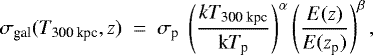 (3)
(3)
where kTp = 2.2 keV and zp = 0.25 are the pivot temperature and redshift, and E(z) = H(z)∕H0 is the normalised Hubble parameter.
The probability distribution function (PDF) of galaxy velocity at a given cluster temperature is taken to be Gaussian with the above dispersion. The ensemble likelihood for the signal component allows for a residual, constant background atop this cluster member signal. The likelihood for the ensemble cluster-galaxy rest-frame velocity sample is thus
![\begin{equation*}\mathcal{L} \ = \ \prod\limits_{i=1}^{n} \left[ \ p \ G(v_{\textrm{gal,}i} | 0, \sigma_{\textrm{gal}}(T_i,z_i)) + \frac{1-p}{ 2 {{v_{\textrm{max}}}}(T_i) } \right], \end{equation*}](/articles/aa/full_html/2018/12/aa31321-17/aa31321-17-eq9.png) (4)
(4)
where G is the Gaussian distribution with zero mean and standard deviation, σgal, vgal is the line-of-sight (LOS) velocity, Eq. (1), and the sum i is over all galaxy-cluster pairs in the spectroscopic sample lying below the maximum cutoff, Eq. (2). The parameter p is the fraction of galaxies that contribute to the Gaussian component, while 1 − p is residual fraction of projected systems that are approximated by a uniform distribution in the signal portion of velocity space.
We maximise this likelihood with respect to the four model parameters, σp, α, β, and p. Below we find that the redshift evolution parameter, β, is both relatively poorly constrained and consistent with zero. We therefore also perform a restricted analysis in which we assume self-similar evolution (SSE), with β = 0.
3.2 Ensemble velocity model in simulations
This model has been tested against simulation by Farahi et al. (2016), using cluster richness instead of X-ray temperature, with several key findings. First, the spectroscopic mass estimate is a nearly unbiased estimator of ⟨ln Mmem|λRM⟩, where Mmem is the mass of the underlying halo that contributes the maximum fraction of the cluster’s photometric member galaxies assigned by redMaPPer. Second, galaxies lying in the signal region consist of a majority coming from the top-ranked, member-matched halo (~ 60%) as well as locally projected galaxies (~40%) lying outside the matched halo. Finally, the main source of systematic uncertainty in the SDSS cluster mass estimate of Farahi et al. (2016) is uncertainty in the magnitude of the galaxy velocity bias.
4 Velocity scaling results
In this section, we present the inferred σgal − kT300 kpc scaling relation for the full cluster sample. The fiducial analysis uses the signal velocity threshold of Eq. (2), an angular limit of r500, and solves for the four degrees of model freedom using the entire sample. Sensitivity tests of the angular and velocity thresholds used in our fiducial treatment are presented in the next section.
We run the Markov chain Monte Carlo (MCMC) analysis module PyMC (Patil et al. 2010) to maximise the likelihood and recover the scaling relation parameters between velocity dispersion of galaxy members and temperatureof hot cluster gas. We assume a uniform priors on all parameters, with the following domain limits: p ∈ [0, 1], σp ∈[50, 1000] km s−1, α ∈ [−10, 10], and β ∈ [−10, 10].
The best-fit parameter values for the fiducial model and the restricted SSE model are given in Table 1. The posterior PDFs of the free parameters are presented in Appendix A.
For the fiducial treatment, the posterior constraint on the slope of galaxy velocity dispersion scaling with temperature is α = 0.63 ± 0.05, is in tension with the self-similar expectation of 0.5. A slope steeper than self-similar could potentially arise from AGN feedback effects on the ICM. Recent simulations including AGN feedback exhibit shifts in the global ICM temperature of halos that are mass-dependent, with larger increases seen at lower masses (Le Brun et al. 2016; Truong et al. 2018). Since the galaxy velocity dispersion is not directly coupled to AGN activity, the impact on the ICM would lead to α >0.5.
We findno significant change in the scaling amplitude with redshift but our constraint is weak, β =−0.49 ± 0.38. Since the fiducial analysis yields no evidence of redshift evolution, it is no surprise that the posterior SSE parameter values are identical to those of the fiducial analysis.
The Gaussian component amplitude, p, is close to, but significantly different from unity. While the value of 0.88± 0.02 is consistent with the 0.916 ± 0.004 value found by Rozo et al. (2015) in their study of SDSS redMaPPer clusters, differences in selection and measurement preclude a direct comparison. Besides sample selection differences, the SDSS galaxy velocities are pairwise with respect to the central galaxy’s velocity, whereas ours are determined by the mean cluster redshift, zc. Some of thedifference could reflect mis-centering, as a larger fraction of mis-centered clusters both reduces p and increases σp (Farahi et al. 2016). We defer detailed modeling of such selection effects to future work.
Normalised velocity residuals about the mean scaling behaviour in the fiducial analysis are shown in Fig. 5. We bootstrap the galaxy sample to compute means and standard deviations of the PDF in 64 bins between − 4 and 4 in v∕σgal, and these are shown as points with error bars in the figure. The line is the model, a Gaussian of zero mean, unit variance and amplitude given by the fiducial best fit plus a constant background.
From Fig. 5, it is evident that our fit is not a good fit to data in the standard chi-squared sense. The normalised velocity PDF structure is very similar to that seen by Rozo et al. (2015) and Farahi et al. (2016) for redMaPPer clusters and simulations, respectively. We find χ2∕d.o.f. = 74∕44 for vgal∕σgal ∈ [−3, 3], which is less than that for the best-fit value found by Rozo et al. (2015) for SDSS redMaPPer clusters,  .
.
While the centrally peaked nature of the normalised velocity PDF remains to be carefully modeled, two potential sources are likely to be important. One is projected large-scale structure; the Farahi et al. (2016) simulations show that only ~ 60% of the galaxies in the signal component of velocity space actually lie within r200 of the halo matched to each member of the cluster ensemble. Another is intrinsic scatter in σgal − TX, which will distort the Gaussian shape. The fact that the χ2∕d.o.f. is smaller for the XXL sample compared to SDSS redMaPPer may reflect the fact that the intrinsic scatter in galaxy velocity dispersion is smaller at fixed temperature than at fixed richness, but differences in selection may also play a role.
Although the best fit is not a good fit to a Gaussian, the simulation of Farahi et al. (2016) show that the derived galaxy velocity dispersion scaling is unbiased with respect to the log-mean value obtained by matching each cluster to the halo that contributes the majority of its galaxy members. Because the galaxy velocities in that simulation are unbiased relative to the dark matter by construction, the virial mass scaling derived from the galaxy velocity dispersion,  , presents an unbiased estimate of the log-mean, membership-matched halo mass of the cluster ensemble. The reader interested primarily in mass scaling estimates can move directly to Sect. 6.
We turnnext to comparing our scaling of galaxy velocity dispersion with gas temperature to previous work, and then explore the robustness of our parameter values in Sect. 5.
Soon after early observations of extended X-ray emission from clusters indicated a thermal gas atmosphere, a dimensionless parameter of interest emerged: the ratio of specific energies in galaxies and hot gas,  , where μ is the mean molecular weight of the plasma and mp is the proton mass (note this beta is fundamentally different from the symbol used in Sect. 3).
Early estimates of this ratio in small observational samples (Mushotzky et al. 1978) and gas dynamic simulations (Evrard 1990; Navarro et al. 1995)yielded βspec ≈ 1, consistent with a scenario in which both components are in virial equilibrium within a common gravitational potential. More recently, this ratio has been explored at high redshift; Nastasi et al. (2014) find βspec = 0.85 ± 0.28 for 15 clusters with z > 0.6.
Figure 6 compares the fiducial scaling relation of this work to previous determinations in the literature. In addition, the dashed (magenta) line shows βspec = 1 assuming mean molecular weight μ = 0.6, appropriate for a metal abundance of 0.3 Z⊙. Shaded regions show 1σ uncertainty on the expected velocity dispersion at a given temperature.
Table 2 summarises the comparison with previous studies. The published scaling relations are re-evaluated at the pivot point of this work to be directly comparable. When appropriate, errors in the published slope are propagated to the normalization error.
The measured slope is consistent between our work and previous works. Wilson et al. (2016) find a slope 0.86± 0.14 for a sample of 38 clusters from the XMM Cluster Survey. Using simulations, however, they show that the orthogonal fitting method on their sample produces a substantial overestimate in slope, by ~ 0.3, in the test shown in their Table 7 and Fig. 9. They caution that their fit overestimates the velocity dispersion of clusters above 5 keV. Similarly Ortiz-Gil et al. (2004) uses the orthogonal fitting method and find a steep slope ~ 1.00 ± 0.16 for a sample of 54 clusters.
If a bias correction is applied, the slope of Wilson et al. (2016) reduces to ~ 0.55, consistent with our findings. We note that a smaller shift of ~0.2 would bring the Ortiz-Gil et al. (2004) result into consistency with self-similarity at the 2σ level. For a heterogeneous sample constructed from the literature, Xue & Wu (2000) report a slope of 0.61± 0.01, consistent with our result.
The velocity dispersion normalizations given in Table 2 at the pivot temperature and redshift are all in good agreement within their stated errors. The 3% fractional uncertainty in our quoted normalization is among the tightest published constraints, comparable to the statistical error of the more heterogeneous sample of Xue & Wu (2000).
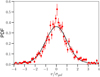 |
Fig. 5 Normalised residuals of galaxy velocity about the mean scaling relation in the fiducial analysis. Red points show the data and the black line is the model, Eq. (4), a mixture of a Gaussian and a uniform distribution. Error bars are calculated by bootstrapping the velocities of the spectroscopic sample, using 64 bins between − 4 and 4 in vgal ∕σgal. See text for discussion of the goodness of fit. |
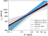 |
Fig. 6 Comparison of the σgal − kT300 kpc scaling relation of this work with prior literature, as labeled. Shaded regions are 1σ uncertainty on the expected velocity dispersion at given temperature. The magenta line is the locus of constant specific energy ratio, |
5 Systematic errors and sensitivity analysis
In this section, we investigate sources of uncertainty in the scaling presented in the previous section, including survey selection and the sensitivity of the posterior parameters to the details of the spectroscopic sample used to define the signal region.
Table 3 summarises the results of the tests presented below. A cursory look at the table indicates that most parameters shift by modest amounts, typically within one or two standard deviations of the fiducial result, with the exception of the Gaussian amplitude, p, discussed further below.
5.1 Temperature estimates
As presented in Sect. 2.1, the XXL temperatures are directly determined for 103 of the 128 clusters in our sample. A natural question to ask is whether our results are sensitive to the temperature estimation method applied to the remaining 25 clusters.
We first note that the 103 systems with measured T300 kpc tend to be more massive at a given redshift, with higher galaxy richness. The higher richness translates into more galaxies with spectroscopy, and it turns out that this subset holds most of the statistical weight of the spectroscopic sample. Within the fiducial r500 aperture, there are 1421 galaxies in the 103 clusters with direct temperatures, compared with 171 galaxies in the 25 clusters with inferred temperatures. So ~90% of the statistical weight comes from clusters with measured temperatures.
As a consistency check, we refit the scaling relation after removing all clusters with inferred temperature from the sample. The parameter constraints remain consistent with our fiducial analysis.
5.2 Angular aperture
The velocitydispersion of dark matter particles in simulations varies weakly as a function of distance from the halo centre (Old et al. 2013), and this effect has been confirmed observationally (Biviano & Girardi 2003). We test the sensitivity of our fit parameters by varying the angular aperture of inclusion by factors of 2±1 from the fiducial value of r500. We note that the size of the sample varies slightly as the aperture is changed. The main change is that a larger aperture induces a larger projection effect, evident from the Gaussian normalization, p = 0.82 ± 0.02 for 2r500 versus p = 0.90 ± 0.02 for 0.5r500. There are modest trends in the other parameters, including a slightly steeper slope α = 0.67 ± 0.07 at 0.5r500, and β is not consistent with 0 at the ~2σ level at 0.5r500, but the statistical power of the sample is insufficient to determine these trends with high precision.
Sensitivity analysis of σgal − kT300 kpc inferred parameters.
5.3 Signal component maximum velocity
Recall that the likelihood model is applied to a subset of all spectroscopic galaxies that lie in the signal region, with rest-frame velocities below a maximum value, vmax(T300 kpc), given by Eq. (2). We test the effect of this maximum by independently varying the amplitude by ± 500 km s−1 (or ± 20%) and the power-law index by ± 0.2. The number of signal galaxies does not vary much with these changes, indicating that our fiducial cut is roughly identifying the caustic edge that separates bound and unbound galaxies in clusters (Miller et al. 2016). All parameters remain within 1σ of their fiducial values as these changes are made.
5.4 Redshift range
We take the pivot redshift in this work, zp = 0.25, and split the full sample into high and low redshift subsets. For these, we do not find statistically significant deviations from the fiducial model parameters. The changes in the normalization, slope, redshift evolution, and parameter p are all less than 1σ. Although, as to be expected, there remains no effective constraints on the redshift evolution factor.
5.5 X-ray selection and Malmquist bias
The aim of our analysis is to produce unbiased estimates of the scaling relations inherent to the population of dark matter halos. Selection by X-ray flux and angular size (Pacaud et al. 2006) can introduce bias in the inferred σgal − kT300 kpc scaling relation if there is non-zero covariance between X-ray selection properties and galaxy velocity dispersion (see Sect. 5.1 in Kelly 2007). Such data sets are said to be “truncated”, and the truncation effects need to be explicitly modeled in the likelihood.
There have not yet been observational estimates of the correlation between galaxy velocity dispersion and X-ray properties at fixed halo mass. Halos in the Millennium Gas simulations of Stanek et al. (2010) show intrinsic correlation coefficients of ~ 0.3 for LX and σDM, where σDM is the velocity dispersion of dark matter particles in the halos. However, translating this estimate into correlations involving σgal projected along the line-of-sight is non-trivial and lies beyond the scope of this work. Redshift-space projection presumably dilutes any intrinsic halo correlation, unless the source of the projected velocity component also carries associated X-ray emission.
The magnitude of potential selection biases can be addressed by simulating the entire process of survey selection and subsequent spectroscopic analysis, along the lines of that done by Farahi et al. (2016) for redMaPPer optical selection. We defer that work to future analysis. From the perspective of halo mass estimation, corrections to the velocity dispersion scaling from sample selection are likely to be smaller than the systematic uncertainty associated with galaxy velocity bias, as discussed below.
6 Ensemble dynamical mass scaling of XXL clusters
As previously noted, Farahi et al. (2016) use sky realizations derived from lightcone outputs of cosmological simulations to show that the mass determined through virial scaling of the ensemble, or stacked, pairwise velocity dispersion offers an unbiased estimate of the log-mean mass of halos matched via joint galaxy membership. Here, we apply this approach to the fiducial velocity dispersion scaling in order to estimate the characteristic mass scale, ⟨ln M200|TX⟩ of XXL clusters as a function of temperature at the pivot redshift, zp = 0.25.
The simulation of Farahi et al. (2016) assumed galaxies to be accurate tracers of the dark matter velocity field, but real galaxies may be biased tracers. To estimate the velocity dispersion of the underlying dark matter from the galaxy redshift measurements, we introduce a velocity bias factor, bv, defined as the mean ratio of galaxy to dark matter velocity dispersion within the target projected r200 region used in our analysis. The normalization of the dark matter velocity scaling with temperature is then
 (5)
(5)
where σp is the galaxy normalization with temperature, Eq. (3).
Following Farahi et al. (2016), we proceed by: i) imposing an external bv estimate to derive the normalization of the dark matter virial velocity scaling with X-ray temperature; then ii) applying the dark mattervirial relation calibrated by Evrard et al. (2008) to determine the scaling of total system mass with temperature.
We use bv = 1.05 ± 0.08 which is an empirical estimate derived from redshift-space clustering of bright galaxies by Guo et al. (2015a). A similar value of 1.06± 0.03 is found in the simulation study of Wu et al. (2013), although that study found galaxy bias slightly below 1 for the brightest galaxies. We note that the peak of distribution of absolute r-band magnitude of selected galaxies in this work is Mr = 21.5 (see Appendix B), which is consistent with the brightest galaxy sample of Guo et al. (2015a). Using a velocity bias of 1.05 ± 0.08 leads to an estimate of the dark matter velocity dispersion at the pivot temperature and redshift,
 (6)
(6)
We note that σp, DM uncertainty has contribution from the bv prior and σp posterior.
The virial scaling of halos in simulations displays a linear relationship between the cube of the dark matter velocity dispersion,  , and a mass measure, E(z)MΔ, where E(z) = H(z)∕H0 is the normalised Hubble parameter. Using Eq. (6) and Table 3 of Evrard et al. (2008) along with h = 0.7, the total mass within r200 at the pivot temperature and redshift is
 (7)
(7)
corresponding to  .
.
The full velocity scaling implies a log-mean mass for the XXL selected cluster sample of
 (8)
(8)
with intercept πT = 0.45 ± 0.24, temperature slope αT = 3α = 1.89 ± 0.15, redshift slope βT = 3β = −1.29 ± 1.14. Recall that this result is based on 300 kpc temperature estimates, T ≡ T300 kpc.
Biviano et al. (2006) have examined the robustness of virial mass estimates in a cosmological hydrodynamic simulation. They find that dynamical mass estimates are reliable for densely sampled clusters (over 60 cluster members). Due to the ensemble technique adapted here, this work does not suffer from sparse sampling of cluster members. Generally speaking, stacking techniques reduce the noise associated with sparse samples, at the price of not constraining the intrinsic scatter.
While we explicitly remove extreme projected outliers in velocity space (see Fig. 3) and account for a residual, constant contribution in the velocity likelihood, it is worth noting that the central Gaussian component has contributions from galaxies that do not lie in the main source halo. While this component retains some degree of projected galaxies, Farahi et al. (2016) shows that the dynamically-derived mass is a robust estimate of log-mean mass at a given observable, in that case ⟨lnM200|λRM, z⟩. While the optical and X-ray samples are selected differently, not enough is known about hot gas and galaxy property covariance to model selection effects precisely. We discussed in Sect. 5.5 why selection effects are unlikely to imprint significant bias into the inferred scaling relation.
6.1 Comparison with previous studies
Figure 7 compares the mass-temperature scaling relation, a dynamical mass estimates, derived in this work with previous studies that use weak lensing (XXL Paper IV) and hydrostatic (Arnaud et al. 2005) mass estimates. Overall, there is a good agreement within the uncertainties.
The data points with error bars are weak lensing estimates of M200 for a subsample of the 100 brightest clusters in XXL (XXL Paper IV). In order to directly compare our MOR with XXL Paper IV and other works, we evaluate all results atz = 0 using h = 1. When shifting the normalization, we assume SSE, βT = 0, yielding πT = 0.09 ± 0.25.
Assuming self-similar redshift evolution, XXL Paper IV estimated the mass−temperature scaling relation using a subsample of 38 out of 100 brightest XXL clusters. To improve their constraint, their sample is complemented with weak lensing mass measurements from clusters in the COSMOS (Kettula et al. 2013) and CCCP (Hoekstra et al. 2015) cluster samples. While the data points plotted in Fig. 7 are taken directly from XXL Paper IV, their published MOR is framed in terms of M500. We therefore convert the normalization to M200 using an NFW profile with concentration c = 3.1, the median value of the XXL Paper IV sample, for which M200∕M500 = 1.4. The slope of the weak lensingrelation lies within ~1σ of the self-similar expectation of 1.5.
The assumption of hydrostatic equilibrium is commonly used to derive masses from X-ray spectral images, and Arnaud et al. (2005) apply this method to a sample of ten nearby, z < 0.15, relaxed clusters in the X-ray temperature range [2−9] keV. The masses are derived from NFW fits to the mass profiles, obtained under the hydrostatic assumption using measurements from the XMM-Newton satellite. We note that they use a core-excised spectroscopic temperature from a 0.1r200 ≤ r ≤ 0.5r200 region. Our result is consistent with that of Arnaud et al. (2005) within their respective errors.
Kettula et al. (2015) combine 12 low mass clusters from the CFHTLenS and XMM-CFHTLS surveys with 48 high-mass clusters from CCCP (Hoekstra et al. 2015) and 10 low-mass clusters from COSMOS (Kettula et al. 2013). From this sample of 70 systems, they measure a mass - temperature scaling relation with slope 1.73 ± 0.19 for M200. When M500 is used, they find a slope of 1.68 ± 0.17 which they argue may be biased by selection. Applying corrections to this (Eddington) bias, they find a slope of 1.52 ± 0.17, consistent with self-similarity.
Table 4 summarises these comparisons, showing the slopes and normalizations scaled to z = 0 for a pivot X-ray temperatureof 2.2 keV. The expected logmass is the largest for weak-lensing proxies, and smallest under the hydrodynamic assumption, but they are statistically consistent within their stated 10−20% errors. The slope derived in this work is statistically consistent with the scalings derived from weak-lensing and hydrostatic techniques. In agreement with prior work, we find a significantly (> 2.5σ) steeper slope than the expected self-similar value of 1.5. A more precise comparison would need to take into account different approaches to measuring X-ray temperature, as well as potential instrument biases (Zhao et al. 2015; Schellenberger et al. 2015). For example, Arnaud et al. (2005) and Kettula et al. (2015) measure core-excised temperatures within r200 while the temperatures used in this work are measured within fixed physical radius. Comparing the non-core excised temperatures of XXL clusters with the core excised temperatures used by Kettula et al. (2013), XXL Paper IV found a mean ratio of  .
.
Several independent hydrodynamic simulations that incorporate AGN feedback, including models from variants of the Gadget code (cosmo-OWLS; Le Brun et al. 2016; Truong et al. 2018) as well as RAMSES Rhapsody-G (Hahn et al. 2017), find slopes near 1.7 for the scaling of mean mass with spectroscopic temperature. These results are in agreement with our finding. We note that the cluster sample used in this work is dominated by systems with kTX < 3 keV, while Lieu et al. (2016)’s cluster sample is dominated by clusters with temperature above 3 keV. Slopes steeper than the self similar prediction for low temperature systems have been noted in preceding observational works as well (e.g., Arnaud et al. 2005; Sun et al. 2009; Eckmiller et al. 2011).
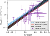 |
Fig. 7 M200 − kT scaling relation from this work (black line and dark shaded region) is compared with published relations given in the legend and Table 4. Shaded regions are the 1σ uncertainty in the expected mass at a given temperature. See the text for more discussion. |
Comparison of the mass normalization, ln A = ⟨ln(M200∕1014 h−1 M⊙) | kTX = 2.2 keV, z = 0⟩, and slope of the mass–temperature determined by the works listed.
6.2 Velocity bias
As in the original application of Farahi et al. (2016) to estimate the mass-richness scaling of redMaPPer clusters, the dominant source of systematic uncertainty in ensemble dynamical mass estimates comes from the uncertainty in the velocity bias correction.
Dynamical friction is a potential physical cause for the velocity bias that would generally drive galaxy velocities to be lower than that of dark matter particles within a halo (e.g., Richstone 1975; Cen & Ostriker 2000; Yoshikawa et al. 2003). On the other hand, clusters that are undergoing mergers tend to have galaxy members with a larger velocity dispersion relative to the dark matter particles (Faltenbacher & Diemand 2006), and merging of the slowest galaxies onto the central galaxy could also tend to drive bv to be greater than one. These competing effects are subject to observational selection in magnitude, colour, galaxy type, star formation activity and aperture which need to be addressed with larger sample size. There is growing observational evidence that velocity bias is a function of the aforementioned selection variables (e.g., Guo et al. 2015a; Barsanti et al. 2016; Bayliss et al. 2017).
The space density of clusters as a function of velocity dispersion also constrains the velocity bias in an assumed cosmology, and (Rines et al. 2007) find bv = 0.94 ± 0.05 and 1.28 ± 0.06 for WMAP1 and WMAP3 cosmologies, respectively. The quoted errors are statistical and based on a sample of 72 clusters in the SDSS DR4 spectroscopic footprint. The study of Maughan et al. (2016) compares caustic masses derived from galaxy kinematics (e.g., Diaferio 1999; Miller et al. 2016) with X-ray hydrostatic masses. Such a comparison yields a measure of relative biases in hydrostatic and caustic methods, and their finding of  for the ratio of hydrostatic to caustic M500 estimates is consistent with unity at the <2σ level. If incomplete thermalization of the intracluster plasma leads hydrostatic masses to underestimate true masses by 20% (e.g., Rasia et al. 2006, and references therein), then the central value of Maughan et al. (2016) indicates that caustic masses would further underestimate true masses. Because of the relatively strong scaling
  , a value bv ≃ 0.9 would suffice for consistency.
Redshift space distortions provide another means to test velocity bias (Tinker et al. 2007). The current constraints from Guo et al. (2015b,a) indicate a magnitude-dependent bias, with  changing from slightly above one for bright systems – the value bv = 1.05 ± 0.08 we employ in Sect. 6 to infer total mass – to slightly below one for fainter galaxies. Oddly, this trend is opposite to that inferred for galaxies from both hydrodynamic and N-body simulations, where bright galaxies are kinematically cooler than dimmer ones (Old et al. 2013; Wu et al. 2013). The recent observational study of (Bayliss et al. 2017) finds a similar trend.
In summary, studies are in the very early stages of investigating velocity bias in the non-linear regime, both via simulations and in observational data. The statistical precision of future spectroscopic surveys, such as DESI (DESI Collaboration 2016), will empower future analyses that may produce more concrete estimates of bv as a function of galaxy luminosity and host halo environment.
Given the current level of systematic error in mass calibration, our ensemble velocity result is consistent with the weak-lensing mass calibration results of XXL Paper IV. Similarly, the weak lensing results of Simet et al. (2017) and Melchior et al. (2017) for redMaPPer clusters agree with the Farahi et al. (2016) estimates. Better understanding of the relative biases of weak lensing, hydrostatic and other mass estimators will shed light on the magnitude of velocity bias in the galaxy population.
7 Conclusion
We model ensemble kinetic motions of galaxies as a function of X-ray temperature to constrain a power-law scaling of mean galaxy velocity dispersion magnitude, ⟨lnσgal|T300 kpc, z⟩ for a sampleof 132 spectroscopically confirmed C1 and C2 clusters in the XXL survey. Spectroscopic galaxy catalogues derived from GAMA, SDSS DR10, VIPERS, VVDS and targeted follow-up surveys provide the input for the spectroscopic analysis. From the kinetic energy, we derive total system mass using a precise dark matter virial calibration from N-body simulations coupled with a velocity bias degree of freedom for galaxies relative to dark matter.
Following Rozo et al. (2015) and Farahi et al. (2016), we employ a likelihood model for galaxy–cluster relative velocities, after removal of high-velocity outliers, and extract underlying parameters by maximising the likelihood using an MCMC technique. The analysis constrains the behaviour of a primary Gaussian component, containing ~ 90% of the non-outlier galaxies, the width of which scales as a power law with temperature, as anticipated by assuming self-similarity (Kaiser 1986).
Based on 1908 galaxy-cluster pairs, we find a scaling steeper than self-similarity,
 (9)
(9)
with σp = 539 ± 16 and α = 0.63 ± 0.05 at a pivot redshift of zp = 0.25. While redshift evolution is included in the likelihood, the data are not sufficiently dense at high redshift to establish a meaningful constraint on evolution.
We identify and characterise several sources of systematic error and study the sensitivity of inferred parameters to the galaxy selection model and assumptions of the stacked model. The method is largely robust (Table 3). It is worth noting that these systematic error sources are generally different from those of other mass calibration methods, such as weak-lensing and hydrostatic X-ray methods, which allows the XXL survey to have an independent estimate of the cluster mass scale.
Employing the precise N-body virial mass relation calibrated in Evrard et al. (2008) coupled with an external constraint on galaxy velocity bias, σgal∕σDM = 1.05 ± 0.08, we derive a halo mass scaling
 (10)
(10)
with normalization, πT = 0.45 ± 0.24, and slopes, αT = 1.89 ± 0.15 and βT = −1.29 ± 1.14.
Within the uncertainties, our result is consistent with mass scalings derived from both weak-lensing measurements of the XXL sample (XXL Paper IV) and provides an independent X-ray analysis using the hydrostatic assumption to obtain mass. But uncertainties in the scaling normalization remain at the level of 10− 25% (see Table 2), and fractional errors in slope are also of order ten percent.
We notethat the dominant source of uncertainty in our mass estimator is not statistical, but systematic uncertainty due to the galaxy velocity bias. Deeper and denser spectroscopic surveys, partnered with sophisticated sky simulations, will enable richer analyses than that performed here. As the accuracy of weak lensing and hydrostatic mass estimates improve, the ensemble method we employ here could be inverted to constrain the magnitude of velocity bias at small scales from future surveys such as DESI (DESI Collaboration 2016). Such an approach has recently been applied to a small sample of Planck clusters by Amodeo et al. (2017).
Larger numbers of spectroscopic galaxies at z > 0.5 are needed to constrain the redshift evolution. In recent hydrodynamic simulations that incorporate AGN feedback, Truong et al. (2018) present evidence for weak redshift evolution in the slope of the mass-temperature scaling relation at z < 1, with stronger evolution at z > 1. Next generation X-ray missions, such as eROSITA (Merloni et al. 2012) and Lynx (Gaskin et al. 2015), will offer the improved sensitivity needed to identify and characterise this population. In the meantime, deeper XMM exposures over at least a subset of the XXL area can be used to improve upon the modest constraints on evolution we obtain using the current 10 ks exposures.
The best practice in comparing the forthcoming, more sensitive observational data with theoretical models will require generating synthetic light-cone surveys from simulations and applying the same data reduction techniques to the models and observations.
An extension that we leave to future work is to properly include temperature errors into the ensemble spectroscopic likelihood model. Richer data will allow investigation of potential modifications to the simple scaling model assumed here, including testing for deviations from self-similarity (in the redshift evolution of the normalization or a redshift-dependent slope, for example) and potential sensitivity to the assembly history or large-scale environment of clusters.
Acknowledgements
XXL is an international project based around an XMM-Newton Very Large Programme surveying two 25 deg2 extragalactic fields at a depth of 5 × 10⁻¹⁵ erg cm−2 s−1 in the [0.5−2] keV band for point-like sources. The XXL website is http://irfu.cea.fr/xxl. Multi-band information and spectroscopic follow-up of the X-ray sources are obtained through a number of survey programmes, summarised at http://xxlmultiwave.pbworks.com/. National Facility which is funded by the Australian Government for operation as a National Facility managed by CSIRO. GAMA is a joint European-Australasian project based around a spectroscopic campaign using the Anglo-Australian Telescope. The GAMA input catalogue is based on data taken from the Sloan Digital Sky Survey and the UKIRT Infrared Deep Sky Survey. Complementary imaging of the GAMA regions is being obtained by a number of independent survey programmes including GALEX MIS, VST KiDS, VISTA VIKING, WISE, Herschel-ATLAS, GMRT and ASKAP providing UV to radio coverage. GAMA is funded by the STFC (UK), the ARC (Australia), the AAO, and the participating institutions. The GAMA website is http://www.gama-survey.org/. This paper uses data from the VIMOS Public Extragalactic Redshift Survey (VIPERS). VIPERS has been performed using the ESO Very Large Telescope, under the “Large Programme” 182.A-0886. This work was supported by NASA Chandra grant CXC-17800360. D.R. is supported by a NASA Postdoctoral Program Senior Fellowship at the NASA Ames Research Center, administered by the Universities Space Research Association under contract with NASA. F.P. acknowledges support by the German Aerospace Agency (DLR) with funds from the Ministry of Economy and Technology (BMWi) through grant 50 OR 1514 and grant 50 OR 1608. The Saclay group acknowledges long-term support from the Centre National d’Études Spatiales (CNES). E.K. thanks CNES and CNRS for support of post-doctoral research.
Appendix A: Posterior parameter distributions
Figure A.1 shows the posterior distributions of the free parameters of the fiducial model5. Posterior PDFs are close to Gaussian, illustrating the convergence of the MCMC chains.
 |
Fig. A.1 Posterior likelihood distributions for σgal − kT300 kpc scaling relation parameters. |
Appendix B: Absoluter-band magnitude of selected galaxies
According to Guo et al. (2015a) the velocity bias runs with the absolute magnitude of selected galaxies. Figure B.1 shows the distribution of absolute r-band magnitude of selected galaxies in this work. We find that the peak of this distribution lies very near Mr = 21.5, which justifies the choice of our prior distribution, bv = 1.05 ± 0.08 found by Guo et al. (2015a) for this magnitude threshold.
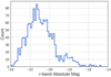 |
Fig. B.1 Thedistribution of r-band absolute magnitude for selected galaxies after applying the fiducial aperture and velocity cuts. |
References
- Adami, C., Mazure, A., Pierre, M., et al. 2011, A&A, 526, A18 [NASA ADS] [CrossRef] [EDP Sciences] [Google Scholar]
- Adami, C., Giles, P., Koulouridis, E., et al. 2018, A&A, 620, A5 (XXL Survey, XX) [NASA ADS] [CrossRef] [EDP Sciences] [Google Scholar]
- Ahn, C. P., Alexandroff, R., Allende Prieto, C., et al. 2014, APJS, 211, 17 [CrossRef] [Google Scholar]
- Allen, S. W., Evrard, A. E., & Mantz, A. B. 2011, ARA&A, 49, 409 [NASA ADS] [CrossRef] [Google Scholar]
- Amodeo, S., Mei, S., Stanford, S. A., et al. 2017, ApJ, 844, 101 [NASA ADS] [CrossRef] [Google Scholar]
- Arnaud, M., Pointecouteau, E., & Pratt, G. W. 2005, A&A, 441, 893 [NASA ADS] [CrossRef] [EDP Sciences] [Google Scholar]
- Barsanti, S., Girardi, M., Biviano, A., et al. 2016, A&A, 595, A73 [NASA ADS] [CrossRef] [EDP Sciences] [Google Scholar]
- Bayliss, M. B., Zengo, K., Ruel, J., et al. 2017, ApJ, 837, 88 [NASA ADS] [CrossRef] [Google Scholar]
- Becker, M. R., McKay, T. A., Koester, B., et al. 2007, ApJ, 669, 905 [NASA ADS] [CrossRef] [Google Scholar]
- Bertschinger, E. 1985, ApJS, 58, 39 [NASA ADS] [CrossRef] [Google Scholar]
- Biviano, A., & Girardi, M. 2003, ApJ, 585, 205 [NASA ADS] [CrossRef] [Google Scholar]
- Biviano, A., Murante, G., Borgani, S., et al. 2006, A&A, 456, 23 [NASA ADS] [CrossRef] [EDP Sciences] [Google Scholar]
- Cavaliere, A., & Fusco-Femiano, R. 1976, A&A, 49, 137 [NASA ADS] [Google Scholar]
- Cen, R., & Ostriker, J. P. 2000, ApJ, 538, 83 [NASA ADS] [CrossRef] [Google Scholar]
- Chiappetti, L., Fotopoulou, S., Lidman, C., et al. 2018, A&A, 620, A12 (XXL Survey, XXVII) [NASA ADS] [CrossRef] [EDP Sciences] [Google Scholar]
- DESI Collaboration 2016, ArXiv e-prints [arXiv:1611.00036] [Google Scholar]
- Diaferio, A. 1999, MNRAS, 309, 610 [NASA ADS] [CrossRef] [Google Scholar]
- Eckmiller, H. J., Hudson, D. S., & Reiprich, T. H. 2011, A&A, 535, A105 [NASA ADS] [CrossRef] [EDP Sciences] [Google Scholar]
- Erben, T., Hildebrandt, H., Miller, L., et al. 2013, MNRAS, 433, 2545 [NASA ADS] [CrossRef] [Google Scholar]
- Evrard, A. E. 1989, ApJ, 341, L71 [NASA ADS] [CrossRef] [Google Scholar]
- Evrard, A. E. 1990, ApJ, 363, 349 [NASA ADS] [CrossRef] [Google Scholar]
- Evrard, A. E., Bialek, J., Busha, M., et al. 2008, ApJ, 672, 122 [NASA ADS] [CrossRef] [Google Scholar]
- Faltenbacher, A., & Diemand, J. 2006, MNRAS, 369, 1698 [NASA ADS] [CrossRef] [Google Scholar]
- Farahi, A., Evrard, A. E., Rozo, E., Rykoff, E. S., & Wechsler, R. H. 2016, MNRAS, 460, 3900 [NASA ADS] [CrossRef] [Google Scholar]
- Foreman-Mackey, D. 2016, The Journal of Open Source Software, DOI: DOI:10.21105/joss.00024 [Google Scholar]
- Gaskin, J. A., Weisskopf, M. C., Vikhlinin, A., et al. 2015, in UV, X-Ray, and Gamma-Ray Space Instrumentation for Astronomy XIX, Proc. SPIE, 9601, 96010J [CrossRef] [Google Scholar]
- Gifford, D., Miller, C., & Kern, N. 2013, ApJ, 773, 116 [NASA ADS] [CrossRef] [Google Scholar]
- Giles, P. A., Maughan, B. J., Pacaud, F., et al. 2016, A&A, 592, A3 (XXL Survey, III) [NASA ADS] [CrossRef] [EDP Sciences] [Google Scholar]
- Guglielmo, V., Poggianti, B. M., Vulcani, B., et al. 2018, A&A, 620, A7 (XXL Survey, XXII) [NASA ADS] [CrossRef] [EDP Sciences] [Google Scholar]
- Guo, H., Zheng, Z., Zehavi, I., et al. 2015a, MNRAS, 453, 4368 [NASA ADS] [CrossRef] [Google Scholar]
- Guo, H., Zheng, Z., Zehavi, I., et al. 2015b, MNRAS, 446, 578 [NASA ADS] [CrossRef] [Google Scholar]
- Guzzo, L., Scodeggio, M., Garilli, B., et al. 2014, A&A, 566, A108 [NASA ADS] [CrossRef] [EDP Sciences] [Google Scholar]
- Hahn, O., Martizzi, D., Wu, H.-Y., et al. 2017, MNRAS, 470, 166 [NASA ADS] [Google Scholar]
- Heymans, C., Van Waerbeke, L., Miller, L., et al. 2012, MNRAS, 427, 146 [NASA ADS] [CrossRef] [Google Scholar]
- Hoekstra, H., Herbonnet, R., Muzzin, A., et al. 2015, MNRAS, 449, 685 [NASA ADS] [CrossRef] [Google Scholar]
- Hopkins, A. M., Driver, S. P., Brough, S., et al. 2013, MNRAS, 430, 2047 [NASA ADS] [CrossRef] [Google Scholar]
- Kaiser, N. 1986, MNRAS, 222, 323 [NASA ADS] [CrossRef] [Google Scholar]
- Kelly, B. C. 2007, ApJ, 665, 1489 [NASA ADS] [CrossRef] [Google Scholar]
- Kettula, K., Finoguenov, A., Massey, R., et al. 2013, ApJ, 778, 74 [NASA ADS] [CrossRef] [Google Scholar]
- Kettula, K., Giodini, S., van Uitert, E., et al. 2015, MNRAS, 451, 1460 [NASA ADS] [CrossRef] [Google Scholar]
- Kravtsov, A. V., & Borgani, S. 2012, ARA&A, 50, 353 [NASA ADS] [CrossRef] [Google Scholar]
- Le Brun, A. M. C., McCarthy, I. G., Schaye, J., & Ponman, T. J. 2016, MNRAS, 466, 4442 [Google Scholar]
- Le Fèvre, O., Vettolani, G., Garilli, B., et al. 2005, A&A, 439, 845 [NASA ADS] [CrossRef] [EDP Sciences] [Google Scholar]
- Le Fèvre, O., Tasca, L. A. M., Cassata, P., et al. 2015, A&A, 576, A79 [NASA ADS] [CrossRef] [EDP Sciences] [Google Scholar]
- Lieu, M., Smith, G. P., Giles, P. A., et al. 2016, A&A, 592, A4 (XXL Survey, IV) [NASA ADS] [CrossRef] [EDP Sciences] [Google Scholar]
- Liske, J., Baldry, I. K., Driver, S. P., et al. 2015, MNRAS, 452, 2087 [NASA ADS] [CrossRef] [Google Scholar]
- Mantz, A. B., Allen, S. W., Morris, R. G., & Schmidt, R. W. 2016a, MNRAS, 456, 4020 [NASA ADS] [CrossRef] [Google Scholar]
- Mantz, A. B., Allen, S. W., Morris, R. G., et al. 2016b, MNRAS, 463, 3582 [NASA ADS] [CrossRef] [Google Scholar]
- Maughan, B. J., Giles, P. A., Rines, K. J., et al. 2016, MNRAS, 461, 4182 [NASA ADS] [CrossRef] [Google Scholar]
- McCarthy, I. G., Schaye, J., Bird, S., & Le Brun A. M. C. 2017, MNRAS, 465, 2936 [NASA ADS] [CrossRef] [Google Scholar]
- Melchior, P., Gruen, D., McClintock, T., et al. 2017, MNRAS, 469, 4899 [NASA ADS] [CrossRef] [Google Scholar]
- Meneghetti, M., Rasia, E., Vega, J., et al. 2014, ApJ, 797, 34 [NASA ADS] [CrossRef] [Google Scholar]
- Merloni, A., Predehl, P., Becker, W., et al. 2012, ArXiv e-prints[arXiv:1209.3114] [Google Scholar]
- Miller, C. J., Stark, A., Gifford, D., & Kern, N. 2016, ApJ, 822, 41 [NASA ADS] [CrossRef] [Google Scholar]
- Mushotzky, R. F., Serlemitsos, P. J., Boldt, E. A., Holt, S. S., & Smith, B. W. 1978, ApJ, 225, 21 [NASA ADS] [CrossRef] [Google Scholar]
- Nastasi, A., Böhringer, H., Fassbender, R., et al. 2014, A&A, 564, A17 [NASA ADS] [CrossRef] [EDP Sciences] [Google Scholar]
- Navarro, J. F., Frenk, C. S., & White, S. D. M. 1995, MNRAS, 275, 720 [NASA ADS] [CrossRef] [Google Scholar]
- Old, L., Gray, M. E., & Pearce, F. R. 2013, MNRAS, 434, 2606 [NASA ADS] [CrossRef] [Google Scholar]
- Ortiz-Gil, A., Guzzo, L., Schuecker, P., Böhringer, H., & Collins, C. A. 2004, MNRAS, 348, 325 [NASA ADS] [CrossRef] [Google Scholar]
- Pacaud, F., Pierre, M., Refregier, A., et al. 2006, MNRAS, 372, 578 [NASA ADS] [CrossRef] [Google Scholar]
- Pacaud, F., Clerc, N., Giles, P. A., et al. 2016, A&A, 592, A2 (XXL Survey, II) [NASA ADS] [CrossRef] [EDP Sciences] [Google Scholar]
- Patil, A., Huard, D., & Fonnesbeck, C. J. 2010, Journal of Statistical Software, 35, 1 [Google Scholar]
- Pierre, M., Pacaud, F., Adami, C., et al. 2016, A&A, 592, A1 (XXL Survey, I) [NASA ADS] [CrossRef] [EDP Sciences] [Google Scholar]
- Rasia, E., Ettori, S., Moscardini, L., et al. 2006, MNRAS, 369, 2013 [NASA ADS] [CrossRef] [Google Scholar]
- Richstone, D. O. 1975, ApJ, 200, 535 [NASA ADS] [CrossRef] [Google Scholar]
- Rines, K., & Diaferio, A. 2010, AJ, 139, 580 [NASA ADS] [CrossRef] [Google Scholar]
- Rines, K., Diaferio, A., & Natarajan, P. 2007, ApJ, 657, 183 [Google Scholar]
- Rozo, E., Rykoff, E. S., Becker, M., Reddick, R. M., & Wechsler, R. H. 2015, MNRAS, 453, 38 [NASA ADS] [CrossRef] [Google Scholar]
- Rykoff, E. S., Koester, B. P., Rozo, E., et al. 2012, ApJ, 746, 178 [NASA ADS] [CrossRef] [Google Scholar]
- Rykoff, E. S., Rozo, E., Busha, M. T., et al. 2014, ApJ, 785, 104 [NASA ADS] [CrossRef] [Google Scholar]
- Schellenberger, G., Reiprich, T. H., Lovisari, L., Nevalainen, J., & David, L. 2015, A&A, 575, A30 [NASA ADS] [CrossRef] [EDP Sciences] [Google Scholar]
- Simet, M., McClintock, T., Mandelbaum, R., et al. 2017, >MNRAS, 466, 3103 [NASA ADS] [CrossRef] [Google Scholar]
- Stanek, R., Rasia, E., Evrard, A. E., Pearce, F., & Gazzola, L. 2010, ApJ, 715, 1508 [NASA ADS] [CrossRef] [Google Scholar]
- Sun, M., Voit, G. M., Donahue, M., et al. 2009, ApJ, 693, 1142 [NASA ADS] [CrossRef] [Google Scholar]
- Tinker, J. L., Norberg, P., Weinberg, D. H., & Warren, M. S. 2007, ApJ, 659, 877 [NASA ADS] [CrossRef] [Google Scholar]
- Truong, N., Rasia, E., Mazzotta, P., et al. 2018, MNRAS, 474, 4089 [NASA ADS] [CrossRef] [Google Scholar]
- Vikhlinin, A., Kravtsov, A., Forman, W., et al. 2006, ApJ, 640, 691 [NASA ADS] [CrossRef] [Google Scholar]
- Wilson, S., Hilton, M., Rooney, P. J., et al. 2016, MNRAS, 463, 413 [NASA ADS] [CrossRef] [Google Scholar]
- Wu, H.-Y., Hahn, O., Evrard, A. E., Wechsler, R. H., & Dolag, K. 2013, MNRAS, 436, 460 [NASA ADS] [CrossRef] [Google Scholar]
- Xue, Y.-J., & Wu, X.-P. 2000, ApJ, 538, 65 [NASA ADS] [CrossRef] [Google Scholar]
- Yoshikawa, K., Jing, Y. P., & Börner, G. 2003, ApJ, 590, 654 [NASA ADS] [CrossRef] [Google Scholar]
- Zhao, H.-H., Li, C.-K., Chen, Y., Jia, S.-M., & Song, L.-M. 2015, >ApJ, 799, 47 [Google Scholar]
Publicly available at http://www.lam.fr/cesam/
Plot produced with the Python package corner.py (Foreman-Mackey 2016)
All Tables
Comparison of the mass normalization, ln A = ⟨ln(M200∕1014 h−1 M⊙) | kTX = 2.2 keV, z = 0⟩, and slope of the mass–temperature determined by the works listed.
All Figures
|
Fig. 1 Spatial distribution of galaxies and clusters in the XXL north field used in this work. Black circles show cluster centres with z ≤ 0.6 with area proportional to temperature. The heat map shows the sky surface density of spectroscopic galaxies lying within a projected aperture of 3r500 around cluster centres. |
| In the text | |
|
Fig. 2 Temperature vs. redshift of the full 132 XXL-N cluster sample. Blue circles are clusters with measured temperature and magenta squares show clusters with inferred temperature. |
| In the text | |
|
Fig. 3 Magnitude of the rest-frame velocity of cluster galaxies, Eq. (1), as a function of cluster temperature. Each dot is one galaxy, and some galaxies appear in the fields of multiple clusters. The black line shows the cut, Eq. (2), that separates the lower signal population from a projected background. Points above the black line are disregarded in our analysis. |
| In the text | |
|
Fig. 4 Frequency distribution of the number of spectroscopic members per cluster within r500 after removing the high-velocity background component using the velocity cut, Eq. (2). |
| In the text | |
|
Fig. 5 Normalised residuals of galaxy velocity about the mean scaling relation in the fiducial analysis. Red points show the data and the black line is the model, Eq. (4), a mixture of a Gaussian and a uniform distribution. Error bars are calculated by bootstrapping the velocities of the spectroscopic sample, using 64 bins between − 4 and 4 in vgal ∕σgal. See text for discussion of the goodness of fit. |
| In the text | |
|
Fig. 6 Comparison of the σgal − kT300 kpc scaling relation of this work with prior literature, as labeled. Shaded regions are 1σ uncertainty on the expected velocity dispersion at given temperature. The magenta line is the locus of constant specific energy ratio, |
| In the text | |
|
Fig. 7 M200 − kT scaling relation from this work (black line and dark shaded region) is compared with published relations given in the legend and Table 4. Shaded regions are the 1σ uncertainty in the expected mass at a given temperature. See the text for more discussion. |
| In the text | |
|
Fig. A.1 Posterior likelihood distributions for σgal − kT300 kpc scaling relation parameters. |
| In the text | |
|
Fig. B.1 Thedistribution of r-band absolute magnitude for selected galaxies after applying the fiducial aperture and velocity cuts. |
| In the text | |
Current usage metrics show cumulative count of Article Views (full-text article views including HTML views, PDF and ePub downloads, according to the available data) and Abstracts Views on Vision4Press platform.
Data correspond to usage on the plateform after 2015. The current usage metrics is available 48-96 hours after online publication and is updated daily on week days.
Initial download of the metrics may take a while.