| Issue |
A&A
Volume 619, November 2018
|
|
|---|---|---|
| Article Number | A180 | |
| Number of page(s) | 19 | |
| Section | Catalogs and data | |
| DOI | https://doi.org/10.1051/0004-6361/201834051 | |
| Published online | 22 November 2018 | |
Reanalysis of the Gaia Data Release 2 photometric sensitivity curves using HST/STIS spectrophotometry⋆
1
Centro de Astrobiología, CSIC-INTA, Campus ESAC, Camino bajo del castillo s/n., 28692
Villanueva de la Cañada, Spain
e-mail: jmaiz@cab.inta-csic.es
2
Departament de Física Quàntica i Astrofísica, Institut de Ciències del Cosmos (ICCUB), Universitat de Barcelona (IEEC-UB), Martí i Franquès 1, 08028
Barcelona, Spain
Received:
8
August
2018
Accepted:
4
September
2018
Context. The second data release (DR2) from the European Space Agency mission Gaia took place on April 2018. DR2 included photometry for more than 1.3 × 10⁹ sources in the three bands G, GBP, and GRP. Even though the Gaia DR2 photometry is very precise, there are currently three alternative definitions of the sensitivity curves that show significative differences.
Aims. The aim of this paper is to improve the quality of the input calibration data to produce new compatible definitions of the G, GBP, and GRP bands and to identify the reasons for the discrepancies between previous definitions.
Methods. We have searched the Hubble Space Telescope (HST) archive for Space Telescope Imaging Spectrograph (STIS) spectra with G430L+G750L data obtained with wide apertures and combined them with the CALSPEC library to produce a high quality spectral energy distribution (SED) library of 122 stars with a broad range of colors, including three very red stars. This library defines new sensitivity curves for G, GBP, and GRP using a functional analytical formalism.
Results. The new sensitivity curves are significantly better than the two previous attempts we use as a reference, REV (Evans et al. 2018, A&A, 616, A4) and WEI (Weiler 2018, A&A, 616, A17). For G we confirm the existence of a systematic bias in magnitude and correct a color term present in REV. For GBP we confirm the need to define two magnitude ranges with different sensitivity curves and measure the cut between them at Gphot = 10.87 mag with a significant increase in precision. The new curves also fit the data better than either REV or WEI. For GRP, our new sensitivity curve fits the STIS spectra better and the differences with previous attempts reside in a systematic effect between ground-based and HST spectral libraries. Additional evidence from color–color diagrams indicate that the new sensitivity curve is more accurate. Nevertheless, there is still room for improvement in the accuracy of the sensitivity curves because of the current dearth of good-quality red calibrators: adding more to the sample should be a priority before Gaia data release 3 takes place.
Key words: surveys / methods: data analysis / techniques: photometric
Table 2 is only available at the CDS via anonymous ftp to cdsarc.u-strasbg.fr (130.79.128.5) or via http://cdsarc.u-strasbg.fr/viz-bin/qcat?J/A+A/619/A180
© ESO 2018
1. Introduction
The second data release (DR2) of the Gaia mission (Prusti et al. 2016) took place in April 2018 (Brown et al. 2018). Gaia DR2 includes photometry for over 1.3 × 10⁹ sources in the three bands G, GBP, and GRP. The G photometry was extracted using point-spread-function (PSF) fitting and has formal uncertainties under 1 mmag for most stars brighter than G = 16. The GBP and GRP magnitudes were obtained through aperture photometry and have larger formal uncertainties, on the order of a few mmag for stars brighter than G = 15, larger than those for G because they are measured just once per transit as opposed to the nine measurements per transit for G. Gaia DR2 constitutes the first all-sky multiband high-precision deep optical photometric survey and as such is likely to be considered an astronomical milestone that will be used as a reference and a calibration source for many studies. However, a high formal precision does not necessarily imply a high accuracy, as one needs to read the “fine print” of how the photometry was obtained to determine the applicability of the published magnitudes and uncertainties. For example, the different nature of the photometry (PSF vs. aperture) leads to G being more accurate than GBP and GRP in crowded (where multiple sources can be included more easily) or nebular (where the background model can be biased) regions (Evans et al. 2018).
Another accuracy issue, which is the main subject of this paper, is the comparison between the observed magnitudes (mphot) and the synthetic ones (msynth) derived from the spectral energy distributions (SEDs) of the sources. In this paper we use Vega magnitudes, as customary for Gaia photometry, and the reader is referred to Appendix B to see how we define the relevant quantities, including the zero points (ZPs) that are one of our results. An accurate definition of the sensitivity curves is especially important for the Gaia photometric system because the three passbands are very broad: G has an effective width1 around 2900 Å (centered around 6400 Å) while those of GBP and GRP are close to 1900 Å (with that of GRP slightly larger) and centered around 5100 Å and 7800 Å, respectively. For comparison, the widths of the Johnson UBV system are 500–700 Å. When doing broad-band photometry of sources with very different intrinsic SEDs and degrees of extinction one needs to integrate each SED to calculate the magnitudes, as a simple evaluation of the flux at a central wavelength does not work. Already for the Johnson UBV system the classical Q approximation to calculate extinction (Johnson & Morgan 1953) breaks down in many practical situations (see Appendix B in Maíz Apellániz & Barbá 2018) due to the non-linearity of the extinction trajectories in the U − B + B − V plane induced by this effect. For Gaia photometry such extinction non-linearities in a color–color plane are even larger and more dependent on the precise definition of the passbands, as we will show later on in this paper.
The first sensitivity curves for the three Gaia passbands were published by Jordi et al. (2010) but those were based on pre-launch data that were later modified. In one of the Gaia DR1 calibration papers, Carrasco et al. (2016) noted that if one used those curves a color term was present in the G photometry and Maíz Apellániz (2017) published a modified sensitivity curve that was able to correct for it. An independent analysis by Weiler et al. (2018) found a very similar sensitivity curve. The Gaia DR1 photometry was affected by a contamination effect caused by water freezing in some optical elements (Prusti et al. 2016) so the Gaia DR2 G data were expected to be characterized by a different sensitivity curve. Indeed, Evans et al. (2018) published not a set but two sets of sensitivity curves for the G, GBP, and GRP photometry in the second data release: one they called DR2 and another one they called REV (for revised, that set was considered the preferred one by the authors). Later on, Weiler (2018) provided a third set that differed from the other two, and that we refer to as WEI. All three by now published sets of Gaia DR2 passbands are based on the same set of calibration sources, the ”Spectrophotometric Standard Stars” (SPSS, Pancino et al. 2012; Altavilla et al. 2015) with the only exception of the WEI GBP passbands, which were derived using CALSPEC (Bohlin et al. 2014, 2017). The SPSS set of calibration spectra is being constructed for the calibration of Gaia, and a first subset of 92 stars was made available for deriving Gaia DR2 passbands. Other spectral libraries, namely CALSPEC, the Next Generation Spectral Library (NGSL, Heap & Lindler 2007), and the library by Stritzinger et al. (2005) have been used for validation purposes by Evans et al. (2018) and Weiler (2018).
The DR2, REV, and WEI results are similar (but not identical) for G: the three sensitivity curves show few differences and agree in their overall shape. They all require a correction for a drift in the zero point of the observed G photometry, as discussed further in Sect. 3 (the corrected G magnitude is denoted G′ here). The results are more different for GBP, as Weiler (2018) found that bright and faint stars follow different sensitivity curves and that there is a jump of 20 mmag in zero point between the two. The WEI sensitivity curves for GBP for the bright and the faint stars both differ strongly in their overall shape from the DR2 and REV passbands. For GRP the differences in shape between the DR2 and REV sensitivity curves and the WEI curve are large, too, although resulting in a small improvement for the SPSS calibration spectra only. Furthermore, Weiler (2018) noted that, while the WEI sensitivity curve for GRP improves the results for the SPSS, Stritzinger, and NGSL libraries, it yields a worse result than the REV passband for the CALSPEC spectra. Weiler (2018) also compared synthetic color–color relationships with observed relationships to test the consistency of a set of sensitivity curves for the three different Gaia passbands. This consistency test showed that the REV set of sensitivity curves fails to reproduce the observed color–color relationships. On the other hand, the WEI sensitivity curves have been designed not only to result in a good reproduction of the observed photometry for each passband individually, but also to reproduce the observed color–color relationships even outside the range in colors covered by the calibration spectra.
In this work, we first compile a new set of calibration spectra based on high-quality HST/STIS optical observations. This set of calibration spectra extends the CALSPEC set significantly, both in number and coverage of different spectral types. In Sect. 2 we describe this set of calibration spectra in detail. We then use the new set of calibration spectra to derive refined sensitivity curves (that will be referred to as MAW from our last names) for all Gaia passbands in Sect. 3. Finally, in Sect. 4 we demonstrate that the calibration data of this work is superior in quality to existing sets of calibration spectra. We also compare synthetic color–color relationships with observed ones, both for main sequence stars and for highly reddened stars, demonstrating that the sensitivity curves derived in this work with a new set of calibration spectra are the most accurate available to date.
2. A new compilation of HST/STIS optical spectra
One of us (J.M.A.) has performed several analyses of the validity of sensitivity curves for different photometric systems (Maíz Apellániz 2005, 2006, 2007, 2017). In those works the main source of spectrophotometric data was NGSL, a spectrophotometric library built from HST/STIS data obtained with the three gratings G230LB+G430L+G750L that covers the 1700–10 200 Å for several hundreds of stars of diverse spectral type. Our original idea for this work was to base it also on NGSL but after several tests we discovered that the quality of their absolute and relative calibrations was not good enough for the purposes of calibrating Gaia DR2 photometry. This issue can be seen, for example, in Figs. 3 and 8 of Weiler (2018), where the dispersion for NGSL stars is higher than for the other three libraries. The likely reason for this problem is that the NGSL data were obtained with a narrow STIS slit, 52 × 0.2, for which absolute flux calibration is difficult to attain.
Not being able to use NGSL, we looked for spectrophotometric substitutes in the HST archive subject to the following criteria:
-
Existence of data for at least the G430L+G750L grating to allow for coverage of the 2900–10 200 Å range. We note that G and GRP have some sensitivity at longer wavelengths but that is small enough that the SED can be interpolated between the STIS data and NIR photometry without a significant bias in the analysis.
-
Use of a wide STIS slit (52 × 0.5 or wider) to avoid flux calibration issues. We note that in a single case below we relax this criterion.
-
S/N large enough in the STIS data for the CTI correction not to introduce large uncertainties.
-
Existence of good-quality Gaia DR2 G, GBP, and GRP photometry.
-
Lack of extended nebulosity around the object and of notorious variability.
1. CALSPEC: This library was already used as a secondary source in our previous works (e.g. Maíz Apellániz 2006) and has been built over the years to calibrate STIS (and other HST instruments) in absolute flux (Bohlin et al. 2017 and references therein). It constitutes the most reliable source, as some of the sources have been observed repeatedly under different conditions and because it uses the widest STIS slit 52 × 2. For this set we downloaded the reduced spectra directly from the CALSPEC web site2. CALSPEC contributes with 63 stars.
2. HOTSTAR: This set is described in Khan & Worthey (2018). It is a hot star extension to NGSL that used the 52 × 0.5 slit, allowing it to be included in this work. In this case we downloaded the raw data from the HST archive and processed it ourselves using the STSDAS package in pyraf. The only exception to the latter is BD −13 4930, whose data is not yet public at the time of this writing; for that star we used the author’s reduction. HOTSTAR contributes with 17 stars.
3. Massa: The third set is that of HST program 13 760 (P.I.: Massa). To our knowledge, no paper has appeared that uses those data. The Massa set uses the 52 × 2 slit and contains 40 stars. As for the previous case, we downloaded the raw data from the archive and processed it ourselves.
4. Other: One problem that is crucial for an accurate calibration of the Gaia DR2 photometry is the use of SEDs covering a wide range in color. In particular the calibration of very red sources of M type require SEDs of such objects in the set of calibration spectra (Weiler et al. 2018). The 120 stars in the three sets described above however only contain stars with a GBP, phot − GRP, phot color less than 1.5, with the only exception of the M-dwarf 2MASS J16553529−0823401 at GBP, phot − GRP, phot = 2.9. It is therefore desirable to include more very red objects in our set of calibrations spectra and to extend it to even redder objects. To address this issue we searched the HST archive for additional red objects with little variability. We found two M dwarfs that satisfy those conditions: BD −11 3759 and Proxima Cen. The first one was observed by HST program 8422 (P.I.: Ferguson) using the 52 × 2 slit. As we did with the previous two sets, we downloaded the raw data from the HST archive and processed it ourselves. For Proxima Cen we used the reduced spectrum provided by Ribas et al. (2017). We note that this second star was observed with the 52 × 0.2 slit but in that paper it was recalibrated in absolute flux using external information.
A fraction of red dwarfs is known to be variable but only 8% of them show variations above 20 mmag (Hosey et al. 2015). We therefore performed checks on the three M-type targets to ensure they are not too strongly variable. We searched the literature for indications of variability. Hosey et al. (2015) lists an amplitude of 13.8 mmag in the V band for BD −11 3759, which is small enough for our purposes. Proxima Cen experiences flux variations due to rotational modulation of surface inhomogenities (Ribas et al. 2017). However, in the optical those have relatively large amplitudes only at short wavelengths. In the V band the amplitude is only on the order of 20 mmag and at longer wavelengths, where we are more interested, is even smaller, a dependence with wavelength that is typical of variable red dwarfs. 2MASS J16553529−0823401 is the faintest of the three red dwarfs and there is less information about variability than for the other two. The AAVSO International Variable Star Index in VizieR lists an amplitude of 45 mmag in V, which likely contains a low-S/N component as the object has a magnitude of 16.7 in that band. On the other hand, 2MASS J16553529−0823401 shows very little variation in the WISE (Cutri et al. 2013) bands, where it is an eighth-magnitude star and has a variability flag of 1 (in a scale of 0–9 with variability starting at 6). Ideally, one would use the variability flag provided by Gaia itself when selecting calibration sources, but this flag will not be available for most of the observed sources until the next data release (DR3). A proxy for variability, however, is the uncertainty on the mean fluxes provided in Gaia DR2. The uncertainty of the mean flux is computed as the standard deviation of the mean flux, which is the standard deviation of the sample of all epoch photometry of a particular source that entered into the computation of the mean flux, divided by the square root of the number of observations (Carrasco et al. 2016). We therefore multiplied the standard deviation of the mean flux with the square root of the number of observations to obtain the standard deviation of the epoch photometry for the three M dwarfs. The standard deviation of the sample of epoch photometry in Gaia DR2 is a very strong function of magnitude and color, though. For a meaningful comparison with typical values for the standard deviation of the epoch photometry we therefore computed the median standard deviation for stars in a small bins in the magnitude-color plane and compared the standard deviation of the three M-dwarfs with the medians of the nearby bins. For all three M dwarfs and for all three Gaia passbands, the standard deviation is smaller than the median standard deviation of stars in the corresponding region of the magnitude-color diagram. The available Gaia DR2 photometry shows thus no indication for significant variability for the three M dwarfs in our set of calibration spectra.
3. Generating the new sensitivity curves
3.1. Theoretical approach
For the determination of the sensitivity curves we use the formalism developed in Weiler et al. (2018). This formalism has already been applied in the computation of the Gaia DR2 sensitivity curves by Weiler (2018), where it has been described in detail. We therefore only provide a sketch of the method here.
The idea of this formalism is to describe a particular sensitivity curve by the sum of two orthogonal functions. One of these functions, denoted the parallel component of the passband, is a linear combination of the principal components of the set of calibration spectra. This function is uniquely defined by the calibration spectra and their corresponding photometric observations. It can be derived by solving a simple set of linear equations for the coefficients of the principal components derived from the calibration spectra. The second function, denoted the orthogonal component of the passband, is unconstrained by the calibration data and is derived in such a way that the passband resulting from adding the parallel and orthogonal component satisfies the physical requirements for the passband (such as non-negativity, being bound to unity, and not oscillating). When deriving several passbands, as is the case here, we can also use the requirement of reproducing observed color–color relationships with the synthetic photometry resulting from the set of passbands as an additional constraint on the choice of the orthogonal component. The derivation of the orthogonal component is performed using an initial guess for the passband and defining a multiplicative linear model for the deformation of the initial guess. For this modification model, we use a linear combination of B-spline basis functions, which is multiplied to the initial guess for the passband. We then choose the coefficients of the B-spline basis functions in such a way that the passband resulting from the multiplication is close to the initial guess, under the constraint that the parallel component of the resulting passband is is agreement with the formal interval of confidence on the parallel component.
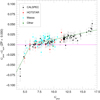 |
Fig. 1. Correction of the systematic errors in G. The horizontal axis is the observed (uncorrected) G magnitude and the vertical axis is the difference between that value and the synthetic G magnitude assuming the G sensitivity curve in this paper and a ZP of 0. The points with error bars show the data, color-coded according to data set, and the dark green solid line shows the fit used to derive the correction proposed in this paper. The size of the error bars is explained in Sect. 4. |
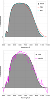 |
Fig. 2. G sensitivity curves. Top: total responses for this work (MAW), Evans et al. 2018 (REV), and Weiler 2018 (WEI) normalized to the same area. Bottom: total response and parallel component for this work with the same scale as on the top panel. |
For a detailed description of this formalism and its practical implementation the reader is referred to Weiler (2018). The sensitivity curves are given in Table 2, separated into their parallel and orthogonal components, respectively. This table is only available at the CDS.
3.2. Sensitivity curve for G
The Gaia DR2 photometry in the G band is affected by systematic errors. Arenou et al. (2018) noticed that G − GBP magnitude shows a systematic trend with G magnitude, which is approximately linear between about 6 and 16 in G. Weiler (2018) and Casagrande & VandenBerg (2018) noticed an approximately linear trend in the difference between the observed G magnitude (Gphot) and the synthetic G magnitude (Gsynth) computed with the REV passband for the CALSPEC spectra. This trend was estimated to be 3.5 ± 0.3 mmag mag−1 and manifests itself in a magnitude dependence of the zero point of the G passband, which can be removed by introducing a correction factor for Gphot.
Here we estimate the correction again excluding sources with G < 6 and G > 16 from our data set. Furthermore, as the Massa data set shows a slight systematic deviation from the remaining calibration spectra, we also exclude them from estimating the trend in G. We find a value of 3.2 ± 0.3 mmag mag−1, thus slightly lower than previous works3. This is the value we use for producing  , the corrected Gphot magnitudes, before computing the sensitivity curves, that is, we assume a relationship:
 (1)
(1)
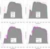 |
Fig. 3. Same as Fig. 2 for GBP. Left panel: bright magnitude range. Right panel: faint magnitude range. |
between  and the number of photoelectrons in the G band, IG, where AZP is the absolute zero point (not to be mistaken with the Vega zero points used elsewhere in this paper). Alternatively,
  can expressed as:
 (2)
(2)
Equation (2) can be used to correct the G magnitudes downloaded from the archive before comparing them with external photometry or synthetic photometry from SEDs. We have no calibration spectra for sources fainter than 16.7 available. The analysis of Arenou et al. (2018) suggests a more complex systematic error for fainter sources, so the linear correction derived in this work may not apply there. Since our data set also contains eleven stars brighter than G = 6 we can produce a correction for them, which we find to be an order of magnitude larger, 27.1 ± 5.8 mmag mag−1, that is: (3)
(3)
The correction for these eleven bright stars is larger because of saturation but is much smaller than the equivalent discussed for Gaia DR1 photometry by Maíz Apellániz (2017), indicating that Gaia DR2 did a much better job with them than Gaia DR1. We note that our eleven stars are all fainter than G = 4, so the correction may fail for brighter stars. Evans et al. (2018) did another saturation analysis and found a correction with the same sign in the range probed here, though its value was slightly larger. In any case, these bright stars were not included in our calculation of the G sensitivity curve. The fits for the two magnitde ranges are shown in Fig. 1.
The G sensitivity curve is computed using six basis functions obtained with the functional principal component analysis of the set of calibration spectra and using the Weiler (2018)G passband as the initial guess. The resulting sensitivity curve is shown in Fig. 2 and compared to the REV and WEI ones. The new curve is very similar to the WEI one, with the main difference between the two in the secondary peak to the left of the Balmer jump which is larger in the new curve. On the other hand, there are significant differences with the REV curve, which has a lower sensitivity in the 7000–8000 Å region and a higher one beyond 9000 Å, that is, it is “redder” (in the sense of being more sensitive at longer wavelengths or, in stellar terms, for cooler temperatures). The consequences of this difference will be explored in the next section.
3.3. Sensitivity curves for GBP
Systematic errors were also previously detected for Gaia DR2 GBP photometry. Arenou et al. (2018) describe a branching of the GBP − GRP versus G − GBP color–color relation for very blue sources, occurring at a G magnitude around 11. This branching results in a “jump” of approximately 20 mmag in GBP. Weiler (2018) confirmed the inconsistency in the GBP photometry by comparing observed and synthetic magnitudes resulting from the REV passband for four different spectral libraries, and located the position of the jump in the range between G magnitudes of 10.47 and 10.99. As the differences between the GBP magnitudes for sources brighter and fainter than the position of the jump depends on color, different sensitivity curves for both sides of the jump are required to describe the GBP photometry. Weiler (2018) thus presented two different passbands for GBP, valid for sources brighter and fainter than 10.99 in G.
The set of calibration spectra used in this work confirms the existence of the inconsistency of the GBP photometry for bright and faint blue sources. In order to better constrain the position of the jump, we used the errors on the mean GBP fluxes. Multiplying these values, provided with Gaia DR2, with the square root of the number of observations results in the standard deviation of the epoch fluxes that entered into the computation of the mean fluxes (Carrasco et al. 2016), which we refer to as the sample standard deviation to clearly distinguish it from the standard deviation of the mean flux. Figure 4 shows this sample standard deviation for all sources with Galactic latitude |b|> 30° for small GBP, phot − GRP, phot color intervals. An abrupt break occurs at a Gphot magnitude of about 10.87, with a clearly increased standard deviation for blue sources fainter than 10.87 mag than for sources brighter than that limit. This jump in the sample standard deviations decreases strongly for redder sources. Assuming that the jump in the sample standard deviations in Gaia’s GBP photometry has the same origin as the jump in the mean magnitudes, we can thus locate the position of the jump more accurately than was done by Weiler (2018) and we obtain a value of 10.87 mag in Gphot.
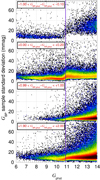 |
Fig. 4. Sample standard deviations of the GBP flux as a function of Gphot for Gaia DR2 stars far from the Galactic Plane (|b|> 30°) for four color ranges GBP, phot − GRP, phot. The histogram shows the logarithm of the number of stars per bin on a common scale for all four panels. We note that the total number of stars per panel increases from the top one to the bottom one. The location of the break is marked with a purple line. |
Although the jump in the sample standard deviations for GBP decreases strongly with increasing color index, it remains detectable up to a GBP, phot − GRP, phot color of about two. When comparing the position of the jump as a function of color in G and GBP, we find that the position in G is far less dependent on color than it is in GBP. We can therefore confirm that the position of the jump in GBP photometry is determined by the G magnitude rather than the GBP magnitude of a source. As the choice of the instrumental configuration (gate and window class) under which a star is observed by Gaia is chosen according to an estimate of the G magnitude, the abrupt jump in GBP at 10.87 mag points to a problem with the calibration of the GBP photometry at different instrumental configurations. The increased sample standard deviation for blue sources fainter than 10.87 mag suggests that the calibration of faint blue sources is less accurate than for the brighter sources, resulting also in the observed systematic color-dependent differences in the mean GBP fluxes and magnitudes.
To take this effect properly into account, we derive two different GBP passbands in this work as was already done in Weiler (2018), valid for sources brighter and fainter than 10.87 mag in Gphot, respectively. The two sensitivity curves were computed using the Weiler (2018)GBP passbands as the initial guess, and using 6 and 5 basis functions for the bright and faint magnitude range, respectively. The resulting bright and faint passbands are shown in Fig. 3 and compared to the REV and WEI ones, noting that the REV result is the same for both magnitude ranges. The same pattern as with G takes place here: the new curves are more similar to the WEI result than to the REV result. The main difference of either MAW or WEI with REV is that REV shows a much more prominent peak for λ < 3800 Å, that is, to the left of the Balmer jump. The peak is weak in the WEI curves and in the faint MAW curve but has almost disappeared from the bright MAW curve. The WEI and MAW faint curves are very similar while the WEI bright curve is slightly “bluer” (in the sense of being more sensitive at shorter wavelengths) than the MAW equivalent.
3.4. Sensitivity curve for GRP
The GRP photometry is less affected by systematic errors than the G and GBP photometry. Weiler (2018) derived a GRP passband that differs clearly from the REV passband. The main effect of the strong change in the RP passband was the removal of a small color tendency in the residuals for the SPSS and Stritzinger spectra. Weiler (2018) however noted that while improving the GRP residuals for the SPSS and Stritzinger spectra, the residuals for the CALSPEC spectra are worse with the WEI passband. Having more calibration spectra available for this work, we can assess the differences between different sets of spectra in more detail in this work.
The GRP passband in this work is computed again with the WEI passband as an initial guess and with 6 basis functions. The solution found in this work is presented in Fig. 5 and compared to the REV and WEI ones. The situation for GRP is different than for G or GBP in the sense that MAW is more similar to REV than to WEI. WEI is more sensitive in the 8000–9000 Å region and less sensitive in the 9500–10 000 Å region, which is the opposite situation to what we find for G, where REV was the one that had those differences in similar wavelength ranges. MAW and REV are not identical and their most importance difference is found below 8000 Å, where REV is redder. In the next section we will explore the consequences of these effects.
Results for the three Gaia bands using the MAW, REV, and WEI sensitivity curves.
4. Testing the new sensitivity curves
We test the MAW sensitivity curves we have generated for the three Gaia DR2 passbands using a similar strategy to the one we recently employed for Gaia DR1 G photometry (Maíz Apellániz 2017) and for the three 2MASS bands (Maíz Apellániz & Pantaleoni González 2018). We check that there are no magnitude or color terms when plotting the difference between observed and synthetic magnitudes and we determine the Vega ZPs (ZPVega, p, see Appendix B for definitions and for how to use the alternative AB or ST systems) for each of the three filters p. We do the same comparison for the REV and WEI sensitivity curves.
For REV and WEI we start by calculating and applying corrections to G in the same way we did for MAW with Eqs. (2) and (3). We then calculate a minimum uncertainty in each band σmin, p (divided by magnitude or color ranges, as appropriate, see below) from the dispersion of the data, as we did in Maíz Apellániz (2006) for Johnson UBV and Strömgren uνby photometry and in Maíz Apellániz (2017) for Gaia DR1 photometry. The minimum uncertainty is the threshold value that should be applied when comparing observed and synthetic magnitudes and depends on the accuracies of the absolute calibration of the spectrophotometric library and the passband characterization as well as on the possible existence of variabilty in the sample. The individual uncertainty for the magnitude of a given star used in this paper is the larger one of (a) the minimum uncertainty for that filter and (b) the published one in each case. We then fit a restricted (slope forced to zero) and an unrestricted linear fit to the difference between (corrected if needed) observed magnitudes and synthetic ones as a function of the GBP, phot − GRP, phot color. The value of the restricted fit yields the ZPVega, p and the slope of the unrestricted fit bp indicates the possible existence of a color term. Our proposed values for ZPVega, p, σmin, p, and bp are given in Table 1.
4.1. G
Our results for G are given in Table 1 and Fig. 6. The left panels of Fig. 6 show that the magnitude dependence is well removed for the three tested sensitivity curves. The right panels of Fig. 6 show that there is no significant color term for either MAW or WEI (bG is less than one sigma from zero) and both solutions provide very similar results, as expected from the comparison of the sensitivity curves (Fig. 2). On the other hand, REV has a strong color term indicated not only by a large value of bG but also by the increasing deviation in the residual  for the three M stars of increasing color. This is a consequence of the redder nature of the REV sensitivity curve previously mentioned. This improvement in the G passband (already present in WEI) remained undetected before, as no sufficiently red calibration sources were available before this work. In fact, the modification of the G passband is highly relevant for getting a good representation of the color–color relationships, as we will see below.
We derive values of σmin, G for the three G sensitivity curves by measuring the dispersion with respect to the ZP in the restricted fit. As saturation effects set in at Gphot = 6, we use that value as the breaking point to define two magnitude ranges. Results are the same for MAW and WEI, 8 mmag for faint stars and 12 mmag for bright ones, with the value for faint stars in REV significantly worse (13 mmag). Those values are much smaller than the 30 mmag (faint) and 74 mmag (bright) derived by Maíz Apellániz (2017) but it is clear now that the reason for such high values was the use of the NGSL spectral library (see above). The σmin, G values are also significantly lower than their equivalents for literature Johnson photometry (20 mmag for B − V and 28 mmag for U − B, Maíz Apellániz 2006) and, furthermore, they refer to the absolute (magnitude) calibration and not to the relative (color) one. Ground-based optical surveys also have higher values of σmin than Gaia: see Padmanabhan et al. (2008) for SDSS and Drew et al. (2014) for VPHAS+. The slightly larger, though still insignificant color term for MAW as compared to WEI results from the Massa spectra, which tend to cluster in a small color range, have a small but systematic offset with respect to the other calibration spectra of this work, as already mentioned in Sect. 3.2. Excluding Massa spectra from the computation, the color term actually becomes zero. The improvement of MAW as compared to WEI is essentially the removal of a small systematic deviation of the CALSPEC spectra at colors around GBP − GRP of 0.3. Considering all of the above and that the formal uncertainty on ZPVega, G is just 1 mmag, we can conclude that the current calibration of the Gaia DR2 G magnitude has an unparalleled quality among deep all-sky photometric survey.
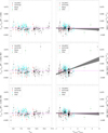 |
Fig. 6. Comparison between the corrected observed G magnitudes and the synthetic G magnitudes as a function of Gphot (left column) and as a function of GBP, phot − GRP, phot (right column). The first, second, and third row show the result for MAW, REV, and WEI, respectively. Data points and error bars are color-coded by data set. The region shaded in gray in the right column shows the 1σ confidence range for the unrestricted fit. |
 |
Fig. 9. Comparison between the (corrected in the G case) observed magnitudes and the synthetic G magnitudes as a function of GBP, phot − GRP, phot for the sample in this paper (black circles) and the Stritzinger sample (red stars). The top, middle, and bottom rows show the results for G, GBP, and GRP, respectively. The left, center, and right columns show the results for MAW, REV, and WEI, respectively. The region shaded in gray shows the 1σ confidence range for the unrestricted fit for the sample in this paper. The region shaded in light orange shows the equivalent for the Stritzinger sample. |
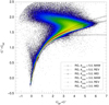 |
Fig. 10. GBP − G′ vs. G′−GRP diagram that includes all stars with 2MASS counterparts, good-quality photometry, and K < 9 mag. The intensity scale is logarithmic. The lines with symbols mark the extinction trajectories of a red giant with Gphot > 10.87 mag using the family of extinction laws of Maíz Apellániz et al. (2014; symbols are spaced by ΔE(4405 − 5495)=0.1 mag and reach to E(4405 − 5495)=5.0 mag) combined in six ways by selecting (a) R5495 = 3 (normal extinction) or R5495 = 5 (H II region extinction) and (b) MAW, REV, or WEI sensitivity curves. See the text for more details. |
4.2. GBP
Our results for GBP are given in Table 1 and Fig. 7. As previously discussed, we have divided our sample into two with a break at Gphot = 10.87 mag, which we also use to divide the calculation of σmin, GBP. As a result, the two subsamples are clearly divided in the left panels of Fig. 7 but are mixed in the right panels.
The jump at Gphot = 10.87 mag manifests itself in the ZPVega, GBP for the two ranges, with differences of 21, 19, and 26 mmag for MAW, REV, and WEI, respectively. There is a large difference in σmin, GBP for bright stars between REV (20 mmag) and either MAW (9 mmag) or WEI (11 mmag). This is a sign of the reality of different GBP sensitivity curves for the two ranges, a factor included in MAW and WEI but not in REV. The difference is smaller for faint stars, indicating that the REV calibration is not as bad there. This is in agreement with the SPSS calibration spectra used to derive the REV passband being dominated by sources in the faint magnitude regime. The small difference between MAW and WEI points toward an improvement of the results in this paper.
Looking at the right panels in Fig. 7 we see a difference between MAW and either REV or WEI. The latter two have a significant negative value of bGBP while that of the former is zero. This indicates that, as it happened with G, the addition of very red sources introduces an improvement in the sensitivity curves that was previously undetected. Furthermore, in this case the improvement takes place in the transition from WEI to MAW while for G it was in the transition from REV to WEI. Considering also that the formal uncertainties on ZPVega, G for the MAW calibration are just 1 mmag (faint) and 2 mmag (bright), we conclude that the current calibration of the Gaia DR2 GBP magnitude has a similar quality to that of G.
We also mention that we attempted an alternative procedure by using a single sensitivity curve for GBP (the faint one) and correcting the bright GBP, phot values into the faint system using a second degree polynomial in GBP, phot − GRP, phot. When doing so, we derived a reasonable transformation but the values of σmin, GBP were higher than the ones described above. Looking into the detailed behavior of the sample, we realized that the reason resided in the different behavior of late-B and early-A stars that is, those with a large Balmer jump, which (for a given extinction) have intermediate GBP, phot − GRP, phot values between those of O/early-B stars and late-type stars. As the most important differences between the bright and faint GBP sensitivity curves are to the left of the Balmer jump, those stars deviate from a correction defined mostly from other types of stars4. Therefore, we decided that alternative procedure (correcting GBP, phot), though attractive due to its simplicity, should be discarded in favor of using different definitions of GBP, synth for different ranges of Gphot.
4.3. GRP
Our results for GRP are given in Table 1 and Fig. 8. In this case we do not need to divide our sample in magnitude ranges, as there is no magnitude-dependent correction (as for G) or need for two different sensitivity curves (as for GBP). However, we divided the sample by color in order to increase the value of σmin, GRP for the three red dwarfs, which play a large role in the calibration of the passband.
The left panels of Fig. 8 do not show trends in magnitude or large differences among the three sensitivity curves and the derived values of σmin, GRP (excluding the three red dwarfs) are also similar (10 mmag for MAW, 11 mmag for the other two). On the other hand, the right panels show significant differences: REV yields a negative value of bGRP, WEI a positive one, and only MAW yields one that is within one sigma of zero. Therefore, the new calibration is an improvement over the previous two but, in this case, the result at this point is more uncertain as it depends mostly on the three red dwarfs. For that reason, we explore the issue in more detail in the next two subsections, where we discuss the effect of using different spectrophotometric libraries and employ additional information from color–color diagrams.
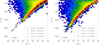 |
Fig. 11. Lower-right region of the GBP − G′ vs. G′−GRP diagram that includes all stars with 2MASS counterparts, good-quality photometry, and K < 11. Left panel: faint stars (Gphot > 10.87 mag). Right panel: bright stars (Gphot < 10.87 mag). The intensity scale is logarithmic. The black and white symbols mark the location of the main sequence using the MAW, REV, or WEI sensitivity curves. The red and white symbols mark the extinction trajectory of a 30 kK main-sequence star using the family of extinction laws of Maíz Apellániz et al. (2014; symbols are spaced by ΔE(4405 − 5495)=0.1 mag). |
4.4. Comparing different spectrophotometric libraries
In order to test the sensitivity curves derived in this work, we compute the synthetic photometry for the spectrophotometric standard stars from Stritzinger et al. (2005) and compare it with the corresponding Gaia DR2 photometry. We omit a comparison with the NGSL because of the large level of uncertainty in these spectra and with the SPSS data set because it has not been published yet. Figure 9 shows the resulting residuals as a function of GBP − GRP color for the MAW, REV, and WEI sensitivity curves and for the three Gaia passbands, respectively.
In all three Gaia passbands, an offset in the residuals from Stritzinger et al. (2005) with respect to our calibration data set is visible, indicating a difference in zero point. For the G passband, all three sets of sensitivity curves result in a similar color trend in the residuals for Stritzinger et al. (2005), with MAW providing the least color dependency. For GBP, the REV passband results in a color dependency for Stritzinger et al. (2005) residuals, which is related to the break in the GBP photometry. All blue Stritzinger et al. (2005) stars with GBP − GRP < 0.6 belong to the bright magnitude regime, which is not well represented by the REV sensitivity curve. The WEI sensitivity curves for GBP remove the color dependency for the Stritzinger et al. (2005) residuals. However, WEI does not fully remove the effects of the break in photometry in the set of calibration spectra used in this work, which may also affect the color dependency of the Stritzinger et al. (2005) residuals. The MAW sensitivity curves describe the calibration sources of this work better than WEI, but at the same time introduce a color dependency in the residuals for the Stritzinger et al. (2005) spectra.
For GRP, the color dependency in the residuals for Stritzinger et al. (2005) spectra is strongest. For the REV sensitivity curves, a clear color dependency of the Stritzinger et al. (2005) residuals is visible. A similar color dependency of the residuals was also observed for the SPSS set of calibration spectra by Weiler (2018), and the WEI sensitivity curve for GRP was constructed to remove this color term from the SPSS residuals. As seen in Fig. 9, the WEI curve also entirely removes the color dependency from the Stritzinger et al. (2005) residuals. The MAW sensitivity curve removes that color term from the calibration spectra of this work, becoming very similar in its overall shape to the REV passband, but it re-introduces the color term in the Stritzinger et al. (2005) data set. We are thus in the situation that the WEI passband provides a better description of the GRP photometric system if the ground-based SPSS and Stritzinger et al. (2005) spectra are used as a standard, while the REV and the MAW sensitivity curves provide a better description if the calibration spectra in this work are used as reference.
The origin for the discrepancy between the different sets of calibration spectra remains unknown. It is however not related to the choice of the orthogonal component of the GRP sensitivity curve. We may use the angle γ as defined in Weiler et al. (2018) to describe the sensitivity of the Stritzinger et al. (2005) spectra to the choice of the orthogonal component of the sensitivity curve. Approximately computing this angle for all Stritzinger et al. (2005) spectra results in very small values below 2° for all spectra in G and GRP, with only one spectrum exceeding 2° in GBP. The synthetic photometry for the Stritzinger et al. (2005) set of spectra is thus strongly dominated by the parallel component of the sensitivity curve with respect to the calibration set used in this work and the systematic difference between the ground-based calibration spectra (SPSS and Stritzinger et al. 2005) and the STIS spectra used for calibration in this work is a small but likely real effect. The difference in shape between the WEI and MAW sensitivity curves for the GRP passband, although appearing large, eventually reflects this small effect.
4.5. GBP-G′ vs. G′-GRP diagrams
A final test of the validity of the different sensitivity curves can be done by comparing the stellar locus in the GBP − G′ vs. G′−GRP observed color–color diagram with the synthetic photometry from stellar models. For this purpose, we cross-matched the Gaia DR2 catalog with 2MASS (Skrutskie et al. 2006) and selected the stars with good-quality photometry and K magnitudes less than 9 or 11, respectively. That selection reduces the dispersion in the color–color diagram and preferentially selects luminous stars, as the bright population in K selects mostly high luminosity and nearby stars for blue colors and mostly red giants for red colors. For the synthetic photometry we use the Maíz Apellániz (2013) solar metallicity grid and the Maíz Apellániz et al. (2014) family of extinction laws5.
Figure 10 shows the GBP − G′ vs. G′−GRP for the sample described above with K < 9 mag. The sample follows a tight correlation in the color–color diagram as one moves diagonally from blue colors to red ones, with an extension that goes from GBP − G′∼4, G′−GRP ∼ 1.6 toward GBP − G′∼0, G′−GRP ∼ 2.1. As described by Evans et al. (2018), the tight correlation that extends from the lower left to the upper right is the real stellar locus while the extension toward the upper left corner is caused by objects with “flux excess”, that is, objects where crowding, nebulosity, or background subtraction introduce contamination in GBP and/or GRP. The lower left part of the stellar locus is populated mostly by low-extinction stars (with some intermediate-extinction O+B stars) with “normal” colors while the central and upper right parts are populated mostly by red giants of increasing extinctions as one moves from center to right. The intrinsic Gaia colors of red giants are relatively well characterized (most of them are bluer than the three M dwarfs in our calibration set) but the extinction trajectories depend on the type of extinction (i.e. the R5495 value for the Maíz Apellániz et al. 2014 family of extinction laws) and the sensitivity curves of the three Gaia passbands. Figure 10 shows the extinction trajectories for a solar-metallicity red giant using two different assumptions for R5495 and the three sets of sensitivity curves described in this paper. The extinction trajectories of the REV sensitivity curves follow very similar paths independently of R5495 (but we note that the position along the trajectory is not the same for a fixed E(4405 − 5495) if R5495 changes) but the trajectories are well below the stellar locus by up to several tenths of a magnitude. This indicates that one or more of the REV sensitivity curves does not correctly describe its passband. Our previous analysis suggests that all three bands have systematic errors for very red objects, with G being the worst of the three. On the other hand, the extinction trajectories for the MAW and WEI passbands show a small dependence with R5495, with the R5495 = 5 case predicting a higher value of G − GRP for a given GBP − G than the R5495 = 3 case. Both MAW and WEI yield trajectories that are consistent with the stellar locus but MAW has the advantage that the center of the stellar locus lies between the R5495 = 3 and R5495 = 5 trajectories, which is the expected result (Maíz Apellániz & Barbá 2018). Therefore, the Gaia color–color diagram for high-extinction stars indicates that the MAW sensitivity curves are slightly better than the WEI ones and significantly better than the REV ones. Another interesting consequence of this analysis is that the extinction trajectories for red giants in the Gaia color–color plane depend more strongly on the definition of the passbands than on the extinction law.
Figure 11 shows the same color–color diagram but for the equivalent sample with K < 11 mag divided into the two subsamples limited by the Gphot = 10.87 magnitude that separates the two GBP sensitivity curves. The left panel shows that for faint stars there are few objects hotter that 10 kK, which is expected because normal stars with K < 11 mag and Gphot > 10.87 mag can be only slightly bluer than Vega in any color formed by filters with most of their sensitivity to the right of the Balmer jump. That panel is dominated by low-extinction AFG stars and the three sets of sensitivity curves describe that stellar locus correctly assuming zero extinction. We note that for faint stars it is possible to use the Gaia colors to differentiate between a zero-extinction A0 main-sequence star and an O star with E(4405 − 5495)∼0.3, as there is a significant separation between the zero-extinction main-sequence stellar locus and the extinction trajectory for hot stars. However, at higher values of E(4405 − 5495) the zero-extinction stellar locus and the extinction trajectory get closer and such a distinction is no longer possible. That is the reason why the stellar locus at high extinctions is so narrow: temperature and extinction become degenerate. The distinction is possible at lower extinctions because of the extra sensitivity of GBP to the left of the Balmer jump.
The right panel of Fig. 11 shows differences with the left panel. In the first place, the diagram is populated up to the extreme of the zero-extinction stellar locus, that is, there are a few low-extinction O and early B stars with K < 11 mag and Gphot < 10.87 mag. That leads to an important difference: the position of the tip agrees with the prediction of the MAW and WEI sensitivity curves but not with that of the REV sensitivity curves. This is another consequence of the reality of the existence of two GBP sensitivity curves. Another difference takes place for redder colors, as the stellar locus is located between the zero-extinction prediction (for any set of sensitivity curves) and the extinction trajectory for hot stars. This indicates that for brighter stars there is a significant fraction of either (a) OBA stars with non-negligible extinction or (b) AF supergiants6. Finally, the switch of GBP sensitivity curve at Gphot = 10.87 mag has the consequence of decreasing the spacing between A0 main-sequence stars with no extinction and O stars with E(4405 − 5495)∼0.3, as the GBP sensitivity to the left of the Balmer jump is lower for bright stars. This is unfortunate, as it makes the use of Gaia photometry by itself to distinguish between populations less useful. In a future paper we will analyze how the combination with 2MASS photometry helps in this issue.
In summary, the GBP − G′ vs. G′−GRP color–color diagrams provide additional evidence that the MAW sensitivity curves are clearly better than the REV ones and that they are slightly better than the WEI ones.
5. Summary and future work
In this work we produced an extension of the CALSPEC set of spectrophotometric standard stars by compiling and re-calibrating suitable HST/STIS observations. The resulting set of calibration spectra was used to derive new sensitivity curves for the three passbands of the Gaia DR2. We used the functional analytic framework by Weiler et al. (2018) for the passband computations.
For the G passband we confirm a systematic magnitude-dependent trend in the photometric system. For the range of magnitudes between 6 and 16, we derive a linear correction of 3.2 mmag mag−1. This correction needs to be applied for an accurate comparison of Gaia DR2 photometry with synthetic photometry. The sensitivity curve for G derived in this work results in a small improvement compared to the WEI sensitivity curve, and a large improvement over the REV one, which shows a strong color term for very red sources.
For the GBP passband we confirm the existence of a color-dependent break in the DR2 photometry that was described by Weiler (2018). This break can be accurately modeled by two different sensitivity curves for GBP, valid for bright and faint sources, respectively. From an analysis of the uncertainties of the GBP fluxes, we can constrain the position of the break better than it was done in Weiler (2018) and we confirm that the break is a result of the G magnitude rather than the GBP magnitude. We therefore present two GBP sensitivity curves, valid for Gphot > 10.87 mag and Gphot < 10.87 mag, respectively. These new sensitivity curves result in a strong improvement as compared to REV, and still a clear improvement as compared to WEI.
For the GRP sensitivity curve we obtained a solution that is similar in its shape to the REV curve, but resulting in an improvement by removing a color dependency in the residuals. However, this solution re-introduces a color dependency in ground-based calibration spectra that was removed by the WEI sensitivity curves. The difference between WEI and the sensitivity curve of this work is thus related to the different sets of calibration spectra used. It is not a lack of constraints on the sensitivity curves in one of the sets of calibration spectra that is causing the difference in shape, but rather a small but systematic difference in spectral shapes.
To verify the consistency of the sensitivity curves for the different passbands, we compared synthetic color–color relationships derived from stellar models with observed color–color relationships. We extend this approach, described in Weiler (2018), by also including high-extinction sources into the comparison. The set of sensitivity curves presented in this work result in a very good agreement with Gaia DR2 color–color relationships over a wide range of colors.
We have demonstrated that HST/STIS observations provide excellent means for calibrating Gaia photometry, allowing for an accuracy better than any other set of spectrophotometric standards. However, there is still room for improvement in the calibration of Gaia DR2 photometry, as the definition of the sensitivity curves for G and GRP depend strongly on three M dwarfs. It is urgent that additional HST spectrophotometry of several tens of very red sources is obtained to solve this deficiency. Once we have seen the diffuclties in producing an accurate calibration for the photometry in Gaia DR2, it is necessary to plan ahead for the calibration of the spectrophotometry in Gaia DR3.
There are different ways to measure the center and width of a passband (see e.g. Sect. 5.1 in Laidler 2005) but that does not affect the argument here.
We have repeated the analysis below with the Cardelli et al. (1989) family of extinction laws and the results are very similar.
We decided not to represent in Fig. 11 the zero-extinction stellar locus for supergiants in order to reduce confusion but for AF stars it is also displaced in the same direction as the extinction trajectory for hot stars. Note, however, that the AF supergiant phase is a short evolutionary phase, so it has few members.
Available from ftp://ftp.stsci.edu/cdbs/calspec/alpha_lyr_stis_003.fits.
See https://www.sdss.org/dr12/algorithms/fluxcal/ for the SDSS case.
Acknowledgments
We thank J.A.C. Escurialensis for his help cum pumilionibus rubris. This work has made use of data from the European Space Agency (ESA) mission Gaia (https://www.cosmos.esa.int/gaia), processed by the Gaia Data Processing and Analysis Consortium (DPAC, https://www.cosmos.esa.int/web/gaia/dpac/consortium). Funding for the DPAC has been provided by national institutions, in particular the institutions participating in the Gaia Multilateral Agreement. J.M.A. acknowledges support from the Spanish Government Ministerio de Ciencia, Innovación y Universidades through grant AYA2016-75 931-C2-2-P. M.W. acknowledges support from the Spanish Government Ministerio de Ciencia, Innovación y Universidades through grants ESP2016-80 079-C2-1-R (MICINN/FEDER, UE), ESP2014-55 996-C2-1-R (MICINN/FEDER, UE), and MDM-2014-0369 of ICCUB (Unidad de Excelencia “María de Maeztu”).
References
- Altavilla, G., Marinoni, S., Pancino, E., et al. 2015, Astron. Nachr., 336, 515 [NASA ADS] [CrossRef] [Google Scholar]
- Arenou, F., Luri, X., Babusiaux, C., et al. 2018, A&A, 616, A17 [Google Scholar]
- Bohlin, R. C.2007, in The Future of Photometric, Spectrophotometric and Polarimetric Standardization, ed. C. Sterken, ASP Conf. Ser., 364, 315 [NASA ADS] [Google Scholar]
- Bohlin, R. C. 2014, AJ, 147, 127 [NASA ADS] [CrossRef] [Google Scholar]
- Bohlin, R. C., Gordon, K. D., & Tremblay, P.-E. 2014, PASP, 126, 711 [NASA ADS] [Google Scholar]
- Bohlin, R. C., Mészáros, S., Fleming, S. W., et al. 2017, AJ, 153, 234 [NASA ADS] [CrossRef] [Google Scholar]
- Brown, A. G. A., Vallenari, A., Prusti, T., et al. 2018, A&A, 616, A1 [NASA ADS] [CrossRef] [EDP Sciences] [Google Scholar]
- Cardelli, J. A., Clayton, G. C., & Mathis, J. S. 1989, ApJ, 345, 245 [NASA ADS] [CrossRef] [Google Scholar]
- Carrasco, J. M., Evans, D. W., Montegriffo, P., et al. 2016, A&A, 595, A7 [NASA ADS] [CrossRef] [EDP Sciences] [Google Scholar]
- Casagrande, L., & VandenBerg, D. A. 2018, MNRAS, 479, L102 [NASA ADS] [CrossRef] [Google Scholar]
- Cutri, R. M., Skrutskie, M. F., van Dyk, S., et al. 2013, VizieR Online Data Catalog: II/328 [Google Scholar]
- Drew, J. E., González-Solares, E., Greimel, R., et al. 2014, MNRAS, 440, 2036 [NASA ADS] [CrossRef] [Google Scholar]
- Evans, D. W., Riello, M., De Angeli, F., et al. 2018, A&A, 616, A4 [NASA ADS] [CrossRef] [EDP Sciences] [Google Scholar]
- Heap, S. R., & Lindler, D. J.2007, in From Stars to Galaxies: Building the Pieces to Build Up the Universe, eds. A.Vallenari, R.Tantalo, L.Portinari, ASP Conf. Ser., 409 [Google Scholar]
- Hosey, A. D., Henry, T. J., Jao, W.-C., et al. 2015, AJ, 150, 6 [NASA ADS] [CrossRef] [Google Scholar]
- Johnson, H. L., & Morgan, W. W. 1953, ApJ, 117, 313 [NASA ADS] [CrossRef] [Google Scholar]
- Jordi, C., Gebran, M., Carrasco, J. M., et al. 2010, A&A, 523, A48 [NASA ADS] [CrossRef] [EDP Sciences] [Google Scholar]
- Khan, I., & Worthey, G. 2018, A&A, 615, A115 [NASA ADS] [CrossRef] [EDP Sciences] [Google Scholar]
- Laidler, V., et al. 2005, Synphot User’s Guide v5.0 (Baltimore: STScI) [Google Scholar]
- Maíz Apellániz, J. 2005, PASP, 117, 615 [NASA ADS] [CrossRef] [Google Scholar]
- Maíz Apellániz, J. 2006, AJ, 131, 1184 [NASA ADS] [CrossRef] [Google Scholar]
- Maíz Apellániz, R. C. 2007, in The Future of Photometric, Spectrophotometric and Polarimetric Standardization, ed. C. Sterken, ASP Conf. Ser., 364, 227 [Google Scholar]
- Maíz Apellániz, J. 2013, Highlights of Spanish Astrophysics, 7, 657 [NASA ADS] [Google Scholar]
- Maíz Apellániz, J. 2017, A&A, 608, L8 [NASA ADS] [CrossRef] [EDP Sciences] [Google Scholar]
- Maíz Apellániz, J., & Barbá, R. H. 2017, A&A, 613, A9 [Google Scholar]
- Maíz Apellániz, J., Evans, C. J., Barbá, R. H., et al. 2014, A&A, 564, A63 [NASA ADS] [CrossRef] [EDP Sciences] [Google Scholar]
- Maíz Apellániz, J., & Pantaleoni González, M. 2018, A&A, 616, L7 [NASA ADS] [CrossRef] [EDP Sciences] [Google Scholar]
- Padmanabhan, N., Schlegel, D. J., Finkbeiner, D. P., et al. 2008, ApJ, 674, 1217 [NASA ADS] [CrossRef] [MathSciNet] [Google Scholar]
- Pancino, E., Altavilla, G., Marinoni, S., et al. 2012, MNRAS, 426, 1767 [NASA ADS] [CrossRef] [Google Scholar]
- Prusti, T., de Bruijne, J. H. J., Brown, A. G. A., et al. 2016, A&A, 595, A1 [NASA ADS] [CrossRef] [EDP Sciences] [Google Scholar]
- Ribas, I., Gregg, M. D., Boyajian, T. S., & Bolmont, E. 2017, A&A, 603, A58 [NASA ADS] [CrossRef] [EDP Sciences] [Google Scholar]
- Skrutskie, M. F., Cutri, R. M., Stiening, R., et al. 2006, AJ, 131, 1163 [NASA ADS] [CrossRef] [Google Scholar]
- Stritzinger, M., Suntzeff, N. B., Hamuy, M., et al. 2005, PASP, 117, 810 [NASA ADS] [CrossRef] [Google Scholar]
- Weiler, M. 2018, A&A, 616, A17 [Google Scholar]
- Weiler, M., Jordi, C., Fabricius, C., & Carrasco, J. M. 2018, A&A, 615, A24 [NASA ADS] [CrossRef] [EDP Sciences] [Google Scholar]
Appendix A: Additional table
Sample used in this paper sorted by GBP, phot − GRP, phot.
continued.
continued.
Appendix B: Zero points and conversions between magnitude systems
We follow the notation of Maíz Apellániz (2007) to write the synthetic magnitudes based on the Vega system for a filter p as: (B.1)
(B.1)
where Pp(λ) is the total-system dimensionless sensitivity curve; fλ, s and fλ, Vega are the star and Vega SEDs, respectively; and ZPVega, p is the filter zero point. One usually tries to define a system with values of zero for the ZPs but, in practice, the ZPs are small but non-zero and have to be calculated from external sources to ensure photometric compatibility across surveys (that is what we have done in this paper, see Maíz Apellániz 2007 for other examples). For consistency with our previous work, we use the Vega spectrum provided by Bohlin (2007)7.
Vega-based magnitude systems have been commonly used in astronomy for decades but they have been critized because they depend on an assumed Vega SED and different authors provide different ones (which makes sense as our knowledge improves over time, see e.g Bohlin 2014). That criticism is valid only as a consistency issue because if one indicates which Vega SED is being used (and makes it available) and defines the ZPs consistently using Eq. (B.1), the magnitudes are correctly defined. If, at one point in the future, somebody comes up with a better Vega SED, the ZPs will change accordingly: (B.2)
(B.2)
and the resulting mVega, p will remain unchanged. Therefore, it is possible to work with the Vega-based definitions on this paper without having to resort to systems based on other reference SEDs.
Nevertheless, some readers may prefer to use the alternative AB system defined as: (B.3)
(B.3)
where fν, AB = 3.63079 × 10⁻²⁰ erg s−1 cm−2 Hz−1 (constant), leading to: (B.4)
(B.4)
On a survey where AB magnitudes are used by default, the values of ZPAB, p will be close to zero (as it is also done for surveys where Vega magnitudes are used, see above) but not exactly so8. However, Gaia uses Vega magnitudes by default so if one imposes the condition mVega, p = mAB, p necessary to compare the synthetic magnitudes calculated this way with the observed ones we find: (B.5)
(B.5)
where mAB, ZP = 0, p(Vega) is the magnitude of Vega in the filter p using the default AB system (the one where ZP = 0). The values of those quantities for the three filters in this paper using the Bohlin (2007) Vega spectral energy distribution are mAB, ZP = 0, G(Vega)=0.125 mag, mAB, ZP = 0, GBP(Vega)=0.044 mag, and mAB, ZP = 0, GRP(Vega)=0.369 mag.
We can do the same analysis for the ST system, whose magnitudes are defined as: (B.7)
(B.7)
where fλ, ST = 3.63079 × 10⁻⁹ erg s−1 cm−2 Å−1 (constant), to reach: (B.8)
(B.8)
where mST, ZP = 0, p(Vega) is the magnitude of Vega in the filter p using the default ST system (the one where ZP = 0). The values of those quantities for the three filters in this paper using the Bohlin & Bohlin (2007) Vega spectral energy distribution are mST, ZP = 0, G(Vega)=0.405 mag, mST, ZP = 0, GBP(Vega)= − 0.137 mag, and mST, ZP = 0, GRP(Vega)=1.124 mag. We note that these values and the equivalent ones for the AB system are not close to zero, as expected, as we have forced the AB and ST magnitudes to be the same as the Vega ones. In other words, these AB (or ST) magnitudes are far from the exact or default AB (or ST) system (defined as the one with ZP = 0).
All Tables
Results for the three Gaia bands using the MAW, REV, and WEI sensitivity curves.
All Figures
|
Fig. 1. Correction of the systematic errors in G. The horizontal axis is the observed (uncorrected) G magnitude and the vertical axis is the difference between that value and the synthetic G magnitude assuming the G sensitivity curve in this paper and a ZP of 0. The points with error bars show the data, color-coded according to data set, and the dark green solid line shows the fit used to derive the correction proposed in this paper. The size of the error bars is explained in Sect. 4. |
| In the text | |
|
Fig. 2. G sensitivity curves. Top: total responses for this work (MAW), Evans et al. 2018 (REV), and Weiler 2018 (WEI) normalized to the same area. Bottom: total response and parallel component for this work with the same scale as on the top panel. |
| In the text | |
|
Fig. 3. Same as Fig. 2 for GBP. Left panel: bright magnitude range. Right panel: faint magnitude range. |
| In the text | |
|
Fig. 4. Sample standard deviations of the GBP flux as a function of Gphot for Gaia DR2 stars far from the Galactic Plane (|b|> 30°) for four color ranges GBP, phot − GRP, phot. The histogram shows the logarithm of the number of stars per bin on a common scale for all four panels. We note that the total number of stars per panel increases from the top one to the bottom one. The location of the break is marked with a purple line. |
| In the text | |
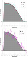 |
Fig. 5. Same as Fig. 2 for GRP. |
| In the text | |
|
Fig. 6. Comparison between the corrected observed G magnitudes and the synthetic G magnitudes as a function of Gphot (left column) and as a function of GBP, phot − GRP, phot (right column). The first, second, and third row show the result for MAW, REV, and WEI, respectively. Data points and error bars are color-coded by data set. The region shaded in gray in the right column shows the 1σ confidence range for the unrestricted fit. |
| In the text | |
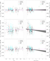 |
Fig. 7. Same as Fig. 6 for GBP. |
| In the text | |
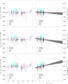 |
Fig. 8. Same as Fig. 6 for GRP. |
| In the text | |
|
Fig. 9. Comparison between the (corrected in the G case) observed magnitudes and the synthetic G magnitudes as a function of GBP, phot − GRP, phot for the sample in this paper (black circles) and the Stritzinger sample (red stars). The top, middle, and bottom rows show the results for G, GBP, and GRP, respectively. The left, center, and right columns show the results for MAW, REV, and WEI, respectively. The region shaded in gray shows the 1σ confidence range for the unrestricted fit for the sample in this paper. The region shaded in light orange shows the equivalent for the Stritzinger sample. |
| In the text | |
|
Fig. 10. GBP − G′ vs. G′−GRP diagram that includes all stars with 2MASS counterparts, good-quality photometry, and K < 9 mag. The intensity scale is logarithmic. The lines with symbols mark the extinction trajectories of a red giant with Gphot > 10.87 mag using the family of extinction laws of Maíz Apellániz et al. (2014; symbols are spaced by ΔE(4405 − 5495)=0.1 mag and reach to E(4405 − 5495)=5.0 mag) combined in six ways by selecting (a) R5495 = 3 (normal extinction) or R5495 = 5 (H II region extinction) and (b) MAW, REV, or WEI sensitivity curves. See the text for more details. |
| In the text | |
|
Fig. 11. Lower-right region of the GBP − G′ vs. G′−GRP diagram that includes all stars with 2MASS counterparts, good-quality photometry, and K < 11. Left panel: faint stars (Gphot > 10.87 mag). Right panel: bright stars (Gphot < 10.87 mag). The intensity scale is logarithmic. The black and white symbols mark the location of the main sequence using the MAW, REV, or WEI sensitivity curves. The red and white symbols mark the extinction trajectory of a 30 kK main-sequence star using the family of extinction laws of Maíz Apellániz et al. (2014; symbols are spaced by ΔE(4405 − 5495)=0.1 mag). |
| In the text | |
Current usage metrics show cumulative count of Article Views (full-text article views including HTML views, PDF and ePub downloads, according to the available data) and Abstracts Views on Vision4Press platform.
Data correspond to usage on the plateform after 2015. The current usage metrics is available 48-96 hours after online publication and is updated daily on week days.
Initial download of the metrics may take a while.