| Issue |
A&A
Volume 619, November 2018
|
|
|---|---|---|
| Article Number | A167 | |
| Number of page(s) | 15 | |
| Section | Stellar structure and evolution | |
| DOI | https://doi.org/10.1051/0004-6361/201833450 | |
| Published online | 20 November 2018 | |
The evolved fast rotator Sargas
Stellar parameters and evolutionary status from VLTI/PIONIER and VLT/UVES⋆, ⋆⋆
1
Université Côte d’Azur, Observatoire de la Côte d’Azur, CNRS, UMR7293 Lagrange, 28 Av. Valrose, 06108
Nice Cedex 2, France
e-mail: This email address is being protected from spambots. You need JavaScript enabled to view it.
2
LESIA, Observatoire de Paris, Université PSL, CNRS, Sorbonne Université, Univ. Paris Diderot, Sorbonne Paris Cité, 5 place Jules Janssen, 92195
Meudon, France
3
Université de Toulouse, UPS-OMP, IRAP, Toulouse, France
4
CNRS, IRAP, 14 Avenue Edouard Belin, 31400
Toulouse, France
5
University of Alcalá, 28871
Alcalá de Henares, Spain
Received:
18
May
2018
Accepted:
13
September
2018
Abstract
Context. Gravity darkening (GD) and flattening are important consequences of stellar rotation. The precise characterization of these effects across the Hertzsprung–Russell (H-R) diagram is crucial to a deeper understanding of stellar structure and evolution.
Aims. We seek to characterize such important effects on Sargas (θ Scorpii), an evolved, fast-rotating, intermediate-mass (∼5 M⊙) star, located in a region of the H-R diagram where they have never been directly measured as far as we know.
Methods. We use our numerical model CHARRON to analyze interferometric (VLTI/PIONIER) and spectroscopic (VLT/UVES) observations through a MCMC model-fitting procedure. The visibilities and closure phases from the PIONIER data are particularly sensitive to rotational flattening and GD. Adopting the Roche approximation, we investigate two GD models: (1) the β-model (Teff ∝ geff β), which includes the classical von Zeipel’s GD law, and (2) the ω-model, where the flux is assumed to be anti-parallel to geff.
Results. Using this approach we measure several physical parameters of Sargas, namely, equatorial radius, mass, equatorial rotation velocity, mean Teff, inclination and position angle of the rotation axis, and β. In particular, we show that the measured β leads to a surface flux distribution equivalent to the one given by the ω-model. Thanks to our results, we also show that Sargas is most probably located in a rare and interesting region of the H-R diagram: within the Hertzsprung gap and over the hot edge of the instability strip (equatorial regions inside it and polar regions outside it because of GD).
Conclusions. These results show once more the power of optical/infrared long-baseline interferometry, combined with high-resolution spectroscopy, to directly measure fast-rotation effects and stellar parameters, in particular GD. As was the case for a few fast rotators previously studied by interferometry, the ω-model provides a physically more profound description of Sargas’ GD, without the need of a β exponent. It will also be interesting to further investigate the implications of the singular location of such a fast rotator as Sargas in the H-R diagram.
Key words: stars: individual: Sargas / stars: rotation / stars: massive / methods: numerical / methods: observational / techniques: interferometric
Based on observations performed at ESO, Chile under program IDs 097.D-0230(ABC) and 266.D-5655(A).
The OIFits files with the VLTI/PIONIER data that we used are publicly available at the JMMC OIDB website service: http://oidb.jmmc.fr/index.html
© ESO 2018
1. Introduction
Sargas is the Sumerian-origin name1 of the evolved, intermediate-mass star θ Scorpii (HIP 86228, HD 159532, HR 6553), the third apparently brightest star (mag V = 1.86) and one of the most southern stars in the Scorpius constellation.
Sargas is classified as an F1III giant by Gray & Garrison (1989, adopted by the SIMBAD database), while other authors classify Sargas as an F0-1II bright giant (e.g., Hohle et al. 2010; Snow et al. 1994; Hoffleit & Jaschek 1991; Samedov 1988). Recently, Ayres (2018) has placed Sargas between F1III and a low-luminosity supergiant of type F0Ib.
Eggleton & Tokovinin (2008) detected a faint companion (visible magnitude 5.36) at a relatively large angular separation of 6.47″. Early on, See (1896) reported the discovery of a companion at a similar separation, (mean values of 6.24″ at a position angle of 321.5°), but much fainter (approx. thirteenth magnitude). Ayres (2018) discusses more recent results concerning the existence of this putative companion.
Despite it being an evolved star, well beyond the main sequence, Sargas is rapidly rotating, with a projected equatorial rotation velocity Veq sin i ∼ 105−125 km s−1 (e.g., Glebocki & Gnacinski 2005; Ochsenbein & Halbwachs 1987). Such a high rotation velocity in an evolved intermediate-mass star is rather atypical, and therefore Sargas provides us with a rare opportunity to further our knowledge on the effects of rotation on post-main sequence stars. In particular, because of its fast rotation rate, Sargas is expected to present (1) geometrical flattening and (2) gravity darkening (GD).
These two effects can be directly constrained by optical/infrared (IR) long-baseline interferometry (OLBI). Indeed, since the beginning of this century, modern stellar interferometers have measured these two consequences of rotation in different stars across the Hertzsprung–Russell (H-R) diagram: Altair (α Aql, A7IV-V; van Belle et al. 2001; Domiciano de Souza et al. 2005; Peterson et al. 2006a; Monnier et al. 2007), Achernar (α Eri, B3-6Vpe; Domiciano de Souza et al. 2003, 2014; Kervella & Domiciano de Souza 2006), Regulus (α Leo, B8IVn; McAlister et al. 2005; Che et al. 2011), Vega (α Lyr, A0V; Aufdenberg et al. 2006; Peterson et al. 2006b; Monnier et al. 2012), Alderamin (α Cep, A7IV; van Belle et al. 2006; Zhao et al. 2009), Rasalhague (α Oph, A5III; Zhao et al. 2009), and Caph (β Cas, F2IV; Che et al. 2011).
The estimated average angular diameter of Sargas is large enough (∼2.5 − 3.3 mas; van Belle 2012; Chelli et al. 2016) to be resolved by the presently operating stellar interferometers, in particular by the ESO-VLTI, which is also well located to observe this southern star. In the following we describe the results of our interferometry-based study of Sargas, adding it to the ongoing list of fast-rotators measured by OLBI. Because the spectral type of Sargas is completely different from these previously observed rapidly rotating stars, the present OLBI study provides a new insight into fast rotation effects in an unexplored region of the H-R diagram.
The interferometric and spectroscopic ESO-VLT(I) data used in this work are described in Sect. 2. The adopted stellar-rotation model is presented in Sect. 3. The physical and geometrical parameters of Sargas estimated in a model-fitting procedure are presented in Sect. 4. A discussion of these results and the conclusions of this work are given in Sects. 5 and 6, respectively.
2. Observations and data reduction
2.1. VLTI/PIONIER
On 11 nights between April and September, 2016, photons from Sargas (and some targets for calibration) were simultaneously collected using four 1.8-m Auxiliary Telescopes (AT) of the ESO-VLTI (Haguenauer et al. 2010) and combined with the PIONIER instrument (Le Bouquin et al. 2011) giving rise to six interference fringe patterns per observation.
These observations, summarized in Table 1, were reduced and calibrated using the standard PIONIER pipeline pndrs (Le Bouquin et al. 2011). After this procedure, each set of six raw fringes from Sargas was converted into a set of six calibrated squared visibilities V2 and four calibrated closure phases CP dispersed over six spectral channels (spectral bin width Δλ = 0.048 μm) within the H band: wavelengths (λ) roughly centered at 1.52, 1.57, 1.62, 1.67, 1.72, and 1.76 μm (small variations of ∼ ± 0.01 μm exist between different observations).
These final, calibrated data of Sargas are provided by the OiDB/JMMC2 service as 30 standard OIFITS files. After removing three individual CP data points flagged as bad in these OIFITS files, our final dataset amounts to 1080 V2 and 702 CP points, that is, 1782 individual interferometric data points and corresponding uncertainties.
Figure 1 shows that the uv-plane of the PIONIER observations is well sampled, both in terms of position angles and projected baselines Bproj, which range from ∼9 to ∼132 m. Such good uv coverage and phase information are important assets in interferometric studies of fast rotators since these objects present non-centrosymmetric intensity distributions. The V2 and CP observables are shown in Figs. 2 and A.1, which are further explained and discussed in the following sections, together with our analysis and modeling results.
Before finishing this section we would like to mention that the putative companion reported by See (1896) and by Eggleton & Tokovinin (2008) should not induce any signature in the PIONIER AT observations since it is located well beyond (⪆30 times) the field-of-view of the instrument. In addition, considering the very faint (thirteenth) magnitude given by See (1896), the putative companion would likely not impact the interferometric data even if it were nearby.
Log of the VLTI/PIONIER observations of Sargas.
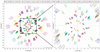 |
Fig. 1. uv coverage (units of spatial frequency) of VLTI/PIONIER observations of Sargas. The VLTI baselines used are identified with different colors (the corresponding AT stations are indicated in the upper legend). The six points per baseline correspond to the six spectral channels of the PIONIER H band observations as described in Sect. 2.1. Projected baselines Bproj range from ∼9 to ∼132 m. A zoom of the central region is shown in the right panel, corresponding to a maximum Bproj of ∼50 m. Image adapted from the OIFits Explorer service from JMMC. |
2.2. VLT/UVES
In addition to the interferometric data we also analyzed reduced spectroscopic data from VLT/UVES, made available by the ESO Science Archive Facility (SAF) in September 2013. We considered four similar spectra obtained on 10 September, 2002, covering the visible wavelength range, from 472.6 to 683.5 nm, with a spectral resolution of ∼74 450. A fifth spectrum taken on the same night was also available but was discarded as bad data, presenting a spurious sinusoidal signal. In our analysis, we choose a subset of the UVES spectra centered on the strong Hα absorption line and covering the range between 643.2 and 669.2 nm, where other weaker lines are also present.
The selected UVES spectra are not absolutely flux calibrated, and in order to use them in our analysis they were normalized and averaged as follows.
-
For the normalization process, the continuum regions were identified by comparing the observational data to synthetic spectra obtained from the AMBRE project (de Laverny et al. 2012, 2013). Twelve wavelength values were selected that were deemed to correspond to continuum points around Hα. To determine the flux at these continuum wavelengths, a moving average was performed on the observational data so that the noise would not affect this continuum flux estimation. Then, for each of the four spectra, the continuum flux over the whole spectral range was obtained from a second-order polynomial fit over these twelve selected continuum points. Finally, this continuum flux was used to normalize both the flux and the associated uncertainties.
-
The average normalized flux Fnorm (and uncertainty σmean) was computed using the weighted average, since the four observed spectra do not have identical signal-to-noise ratios (S/N; values ranging from ∼360 to ∼470).
-
The four normalized spectra do not perfectly overlap, even though the same normalization procedure was applied. This is because the continuum level is never identical among distinct observed spectra. The final total error on Fnorm (σFnorm) was therefore estimated by adding (quadratically) the standard deviation of the four spectra relative to Fnorm to the uncertainty σmean. These two uncertainties are of the same order of magnitude.
To overcome this difficulty we considered a limited subset of 257 selected wavelengths, which ensured an acceptable computation time for the models, and at the same time preserved the high-spectral-resolution information in the UVES data. Indeed, the observed spectral lines are wide because of Sargas’ high Veqsini, which allowed us to determine this limited wavelength subset while keeping the physical information in the line profiles. This selected spectrum was also spectrally shifted based on the theoretical wavelength value of the Hα line in order to be consistent with our analysis using modeled (not shifted) spectra. The 257 selected wavelengths homogeneously sample the whole considered spectral range (around Hα), with a denser sampling (by a factor ≃1.6) in the regions of photospheric absorption lines.
The final normalized and selected UVES spectrum around Hα considered in this work is shown in Figs. 3 and A.2, which are further explained and discussed in the following sections.
Before continuing we note that, after conducting our work using the reduced spectra released in 2013, a new release was delivered by ESO SAF in October 2017, which included some improvements in their processing method. Having already done our analysis with the 2013 release, we decided to compare the two releases to check whether the analysis had to be done again with the new release or not. We found that for almost the whole considered spectral range around Hα, the relative difference between the two spectra did not exceed 0.25%. The difference reached 2.5% at very few (∼3 − 4) narrow wavelength regions, which also correspond to regions where the errors associated with the spectra are the highest. This led us to conduct our analysis with the spectra of the first release, since the small discrepancies between the two releases would hardly affect the results of this work.
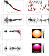 |
Fig. 2. Comparison between interferometric observables from PIONIER (black dots with error bars) and from the β-best-fit model (red squares) presented in Table 2: squared visibilities V2 as a function of both spatial frequencies and baseline position angles (PA), and closure phases as a function of spatial frequencies defined at the longest baseline of the corresponding triangle. The error-normalized residuals of these comparisons are also shown (black dots); horizontal lines indicate the 0 (dashed line) and ±3σ (dotted line) reference values. The vertical dashed lines in the plots with PA abscissas indicate the PAs of the sky-projected rotation axis for the visible (PArot) and hidden (PArot − 180°) stellar poles. The two images at the bottom right show one specific intensity map, computed at the 1.62 μm spectral channel of the PIONIER data, and the Teff map corresponding to this β-best-fit model. These images are not rotated by PArot, i.e., they do not represent the star in sky coordinates. |
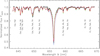 |
Fig. 3. Comparison between the normalized flux from UVES (black dots with error bars) and from the β-best-fit model (red curve) presented in Table 2. The spectra shown span ∼26 nm centered on the Hα line, where the main atoms and ions contributing to the strongest absorption lines have been identified. These observations correspond to 257 selected wavelengths, which homogeneously sample the whole relevant spectral range, as shown by the data points. The thin curves correspond to normalized model fluxes for the same β-best-fit model, but where we have fixed Teff to Tp (blue) and Teq (green) over the whole photosphere (model without GD, i.e., β = 0). Clearly the complete best-fit model, with GD, better reproduces the observed spectral lines compared to the simpler model spectra computed with β = 0. |
3. Stellar-rotation model
3.1. Flattened Roche-star
To interpret the foregoing observations of Sargas we adopt a stellar-rotation model similar to the one used by Domiciano de Souza et al. (2014). The photospheric structure is given by the Roche model: uniform (rigid) rotation with constant angular velocity Ω and mass M concentrated at the center of the star. This is a very good approximation for such an intermediate mass, fast-rotating evolved star like Sargas.
The rotationally flattened stellar photospheric surface follows the Roche equipotential so that the stellar radius R as a function of the colatitude θ can be expressed as (e.g., Kopal 1987; Domiciano de Souza et al. 2002, and references therein)
![Mathematical equation: $$ \begin{aligned} R(\theta ) = R_{\mathrm{eq} }(1-\epsilon ) \frac{\sin \left[\frac{1}{3}\arcsin \left( \frac{\Omega }{\Omega _{\mathrm{c} }}\sin \theta \right) \right] }{\frac{1}{3}\left( \frac{\Omega }{\Omega _{\mathrm{c} }}\sin \theta \right)},\end{aligned} $$](/articles/aa/full_html/2018/11/aa33450-18/aa33450-18-eq2.gif) (1)
(1)
where the flattening parameter ϵ is given by
 (2)
(2)
In the foregoing equations, G is the gravitational constant, Req and Rp are the equatorial and polar radii, Veq(=ΩReq) is the equatorial rotation velocity, and Ωc is the critical angular velocity of the Roche model, that is,
 (3)
(3)
with Rc(=1.5Rp) being the critical equatorial radius. At critical rotation, ϵ reaches its maximum value of 1/3. We also introduced the critical equatorial velocity Vc = ΩcRc. The ratio Ω/Ωc in Eq. (1), and the corresponding ratio Veq/Vc can be expressed in terms of ϵ as
 (4)
(4)
The Keplerian orbital angular and linear velocities (Ωk and Vk) are also often used to scale Ω and Veq:
 (5)
(5)
where
 (6)
(6)
From the gradient of the Roche potential we can derive the surface effective gravity, which, in spherical coordinates (unit vectors  ), is given by
 (7)
(7)
The ratio between the equatorial geq and polar gp surface effective gravities can be expressed as (cf. Domiciano de Souza 2014)
 (8)
(8)
We note that the stellar flattened shape and effective gravity in the Roche model are totally defined by Req, M, and Veq.
3.2. Gravity darkening
To analyze Sargas we consider two distinct GD prescriptions, which have been used in recent interferometry-based works on fast rotators. Both prescriptions assume that the stellar shape is given by the Roche model described in Sect. 3.1.
3.2.1. β-model
The first GD prescription is the β-model, which is a generalization of the classical von Zeipel law (von Zeipel 1924). The local, photospheric radiative-flux is assumed to follow a power law of the local effective gravity geff, namely
 (9)
(9)
where σ is the Stefan-Boltzmann constant. This equation allows us to compute the local effective temperature Teff as a function of geff = ∥geff∥, but adds two new parameters, namely the GD exponent β and the coefficient C. Instead of using C, we prefer to adopt the average effective temperature  , which is more directly related to observable quantities.
  and C are related to the stellar luminosity L by
 (10)
(10)
where  is the total stellar photospheric surface area, that is, the area of the Roche surface defined in Eq. (1), and
  is the radius of an equivalent spherical star of photospheric surface S⋆. In the above equation we have also introduced the β-model average gravity
  , which is not a new quantity since it is obtained from Eqs. (1) and (7). We can now express Teff in the β-model as
 (11)
(11)
The β-model is thus totally defined by five parameters, that is, three parameters describing the Roche model and two new parameters for the GD: Req, M, Veq,  , and β.
3.2.2. ω-model
As a second prescription for the GD, we adopt the ω-model (Espinosa Lara & Rieutord 2011), which is also based on a Roche-star model and is detailed in Rieutord (2016). Compared to the von Zeipel’s law, which introduces the ad hoc parameter β, the ω-model is based on the physical assumption that the flux and the effective gravity are anti-parallel in a radiative envelope. Namely, one assumes that
 (12)
(12)
where f(r, θ) is a universal function that only depends on the parameter ω (or, alternately, ϵ) given by Eq. (5). The full ESTER two-dimensional (2D) models of rapidly rotating early-type stars have shown that the assumption expressed by Eq. (12) is actually a very good approximation even for very distorted stars, since the angle between the two vectors never exceeds half a degree (Espinosa Lara & Rieutord 2011). With this assumption, the ω-model introduces no extra parameters and can give ω immediately.
From Eq. (12) we deduce the following relation between the local flux (or Teff) and geff.
 (13)
(13)
Here, r(θ) is the scaled (by Req) radial distance of the stellar surface and the function f(r, θ) is determined from the flux conservation equation ∇ ⋅ F = 0. Espinosa Lara & Rieutord (2011) show how to solve this equation to obtain Teff in the ω-model (their Eq. (31)):
 (14)
(14)
where ϑ is given by
 (15)
(15)
at each colatitude (see Rieutord 2016, Eq. (18)).
As before, we use the average effective temperature  to rewrite the equation above as
 (16)
(16)
The parameter  is the average gravity, given by
 (17)
(17)
which is distinct from  , but still derived from previously defined quantities.
The ω-model requires only  as an additional parameter to the three Roche-star parameters (no β exponent is needed). It is therefore completely defined by Req, M, Veq, and
  .
.
Although the GD exponent β is not required in the ω-model, it is useful to define an equivalent exponent βω for a future comparison with the β-model. There are different ways to define βω and here we consider the expression from (Rieutord 2016, Eq. (28)), rewritten in terms of ϵ thanks to Eq. (5):
![Mathematical equation: $$ \begin{aligned} \beta _\omega&= \frac{\ln \left( T_{\mathrm{eq} }/T_{\mathrm{p} } \right)}{\ln \left( { g}_{\mathrm{eq} }/{g}_{\mathrm{p} } \right)} =\frac{1}{4} - \frac{1}{6} \frac{\ln \left(\frac{1-3\epsilon }{1-\epsilon } \right) +2\epsilon (1-\epsilon )^2}{\ln \left[(1-\epsilon )(1-3\epsilon )\right]} \nonumber \\&\simeq \frac{1}{4} - \frac{1}{3} \epsilon , \end{aligned} $$](/articles/aa/full_html/2018/11/aa33450-18/aa33450-18-eq31.gif) (18)
(18)
where the approximate result in the last line above is a useful first-order approximation for βω.
In the previous equation, the ratio geq/gp is given by Eq. (8) and the equatorial to polar effective temperatures ratio is given by (cf. Espinosa Lara & Rieutord 2011; Domiciano de Souza 2014)
 (19)
(19)
3.3. Images and observables with CHARRON
Both the β- and the ω-models were implemented in our IDL-based program CHARRON3, briefly described here. A detailed description is given by Domiciano de Souza et al. (2002, 2012) and Domiciano de Souza (2014).
In CHARRON, the 2D Roche photosphere is divided into nearly equal surface area elements (∼50 000). From the input parameters and equations defining the β- and the ω-models, CHARRON associates, with each area element, a set of relevant physical quantities, such as, effective temperature Teff(θ) and gravity geff(θ), rotation velocity V(θ)( = ΩR(θ)), normal surface vector, among others.
From these physical quantities, CHARRON computes wavelength(λ)-dependent intensity maps of the visible stellar surface (images) by associating a local specific intensity I with each surface area element. Each local I depends on several parameters: geff, Teff, metallicity, microturbulent velocity, rotation velocity projected onto the observer’s direction (Vproj), and others. To compute specific intensity maps it is also necessary to define the observer’s position relative to the modeled star. This requires the introduction of three “position” parameters, namely, the stellar distance d, the rotation-axis inclination angle i, and the position angle of the sky-projected rotation axis PArot (counted from north to east until the visible stellar pole).
In this work, the CHARRON images are thus obtained by associating, with each surface grid element j, a local specific intensity from a plane-parallel atmosphere model, so that
 (20)
(20)
where λ is Doppler-shifted to the local Vproj, j, and μj is the cosine between the normal to the surface grid element and the line-of-sight (limb-darkening is thus included). Both Vproj, j and μj depend on the inclination i.
The Ij are obtained by interpolating grids of synthetic spectra pre-calculated for different values of geff, Teff, and λ. To model the high-resolution UVES spectra we used the synthetic fluxes grid from the AMBRE project (de Laverny et al. 2012, 2013) obtained from the MARCS model atmospheres for late-type stars (Gustafsson et al. 2008). Since the AMBRE spectra do not cover the IR domain, we adopted the ATLAS9 grid of low-spectral-resolution fluxes from Castelli & Kurucz (2004) in order to model the low-spectral-resolution PIONIER observations. We checked that the spectra from these two models agree well in their common domain (visible).
We adopted synthetic spectra computed with solar abundance for Sargas since it is a nearby star and is not known to be chemically peculiar. This choice is justified by the chemical composition measurements from Hinkel et al. (2014), who report abundances very close to solar. In particular, these authors give [Fe/H] = 0 and [Ti/Fe] = 0, which are elements contributing to most UVES spectral lines considered in this work. Samedov (1988) also reports a chemical composition close to but somewhat lower than the solar one. Moreover, we note that small deviations from the adopted chemical composition do not significantly impact the low-spectral-resolution PIONIER data, which are the main observational set in our analysis.
The adopted AMBRE and ATLAS9 spectral fluxes were computed with microturbulent velocities ξt of 1 and 2 km s−1, respectively. A precise measure of this parameter on a fast rotator such as Sargas is not easy because line broadening is completely dominated by rotational Doppler broadening. We thus estimated ξt for Sargas from the empirical relation of Adibekyan et al. (2015, Eq. (A1)) for evolved K and G stars (similar but slightly colder than Sargas): ξt ≃ 1.5−2.0 km s−1. This estimation confirms the expected low value of ξt for Sargas and justifies the adopted value. In any case, this parameter does not play an important role in a fast rotator such as Sargas since (1) Veq ∼ 50ξt (i.e., line broadening is dominated by rotation); and (2) ξt has negligible influence on the broad band interferometric observations, both because it hardly affects the continuum spectral distribution and because it does not influence the overall shape (size) or alter the large-scale surface distribution of the star.
Since only the fluxes F of the AMBRE and ATLAS9 spectral grids are available, and not the specific intensities, we converted F into a corresponding grid of surface-normal specific intensities I(μ = 1) using the four-parameter non-linear limb-darkening law from Claret (2000; his Eq. (6)). By interpolating I(μ = 1) as explained above and using Claret’s limb-darkening law, CHARRON computes Ij at each stellar surface area element to generate images (sky-projected specific intensity maps); examples are shown in Figs. 2 and A.1, which are presented in the following sections.
The CHARRON-simulated observed fluxes and interferometric observables (e.g., visibilities and closure phases) are directly obtained from the Fourier transform of these images (e.g., Domiciano de Souza et al. 2002).
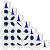 |
Fig. 4. Results obtained from the fit of the β-model to the interferometric and spectroscopic observations Sargas using the CHARRON and emcee codes (further details in the text). The figure shows one- (histograms) and two-dimensional projections of the posterior probability distributions obtained from the fitted parameters. The median (dashed lines) and uncertainties (dotted lines) obtained from the histograms for each fitted parameter are also indicated over the plots and correspond to the values given in Table 2. In the two-dimensional plots lower (higher) χ2 values correspond to darker (lighter) symbols; these 6000 points correspond to the converged final results of the MCMC model-fitting with emcee. |
4. Sargas’ parameters from MCMC model-fitting
In this section, we constrain the input parameters of the β- and the ω-models by comparing the CHARRON observables to the real observations of Sargas described in Sect. 2: H-band squared visibilities V2, closure phases CP from PIONIER, and normalized spectral flux Fnorm (around Hα) from UVES. The use of these three distinct types of observations strengthen the constraints imposed on the model parameters. As discussed in Appendix B, the bandwidth smearing effect can be neglected in the interferometric data analyzed in this work.
In a procedure similar to the one adopted by Domiciano de Souza et al. (2014), we performed the comparison model observations through a model-fitting approach using the emcee code (Foreman-Mackey et al. 2013)4. This code is a Python implementation of the Markov chain Monte Carlo (MCMC) ensemble sampler with affine invariance, which was proposed by Goodman & Weare (2010).
Given a likelihood function relating model and data, emcee draws samples of the posterior probability density function (PDF), even for large parameter-space dimensions. From these samples one can build histograms of the free parameters of the model and then measure their expectation values and uncertainties. Prior information on the model parameters can also be taken into account by emcee.
In this work, the measurement errors on V2, CP, and Fnorm are assumed to be independent and normally distributed, so that the likelihood function is proportional to exp(−χ2/2), where the chi-squared χ2 has its usual definition.
As described in Sect. 3, the input parameters for the β- and ω-models are Req, M, Veq,  , i, PArot, d, and β as an additional parameter for the β-model. All these quantities were considered as free parameters to be fitted with emcee, except the distance, which was incorporated as a prior, following the value from Hohle et al. (2010, based on revised Hipparcos parallaxes) : d = 91.16 ± 12.51 pc. Sargas’ distance is not given in the Data Release 2 (DR2) of the Gaia mission.
Because ∼10 − 20 s are required for CHARRON to simulate one complete set of Sargas observables on a standard desktop computer, the emcee model-fitting was performed in two steps so that it could finish in a reasonable time (a few days).
In a first step, emcee runs with a limited number of walkers (100) in a long burn-in and final phases (350 and 50 iterations, resp.). This ensures convergence of emcee within the burn-in phase and allows a first estimate of expectation values and uncertainties σ. The free parameters were allowed to span a relatively large range of the parameter space. This large, but still limited, parameter space domain was determined based on some preliminary tests with CHARRON and LITpro/JMMC (Tallon-Bosc et al. 2008), and on values from previous works. Since not all parameter have been measured in the past or were measured with distinct precisions, they were initialized following uniform distributions over the parameter space domain.
A second step was then performed with a larger number of walkers (400), but shorter burn-in and final phases (100 and 15 iterations resp.). In this step the free parameters were centered on the expected values (median) found in the first step, and were restricted to span a much more limited region of the parameter space (typically from ∼ − 7σ to ∼7σ relative to the median), again with initial uniform distributions. Convergence was then still attained during burn-in, and the histograms on the fitted parameters could be built from the final 15 emcee iterations (total of 6000 points).
The best-fitting parameter values (median) and uncertainties obtained from the CHARRON-emcee fit of the β- and the ω-models to the observations are presented in Table 2. Several derived stellar parameters are also given in this table. We note that Sargas’ parameters measured from the β- and ω-models are in very good agreement (within their uncertainties).
The direct comparisons between the interferometric and spectroscopic observables and the β-best-fit model are shown in Figs. 2 and 3. The corresponding images for the ω-model are very similar and are given in Figs. A.1 and A.2. The signature of rotational flattening is clearly seen in the V2 curves (GD also influences the V2). The CP plots clearly indicate the signature of GD, revealed by the departure from zero seen at high spatial frequencies.
GD also has a subtle influence on the spectral flux, and in order to better appreciate this we have added the spectra of two β models with identical best-fit parameters, but with Teff fixed (β forced to 0) to the two extreme values Tp and Teq. The spectra from these fixed Teff models are included in Fig. 3, where one can see that they are less effective in reproducing the whole set of spectral features than the complete best-fit model with GD.
The reduced chi-squared of the best-fit for both models is χr = χ2/d.o.f. = 5.4, which is composed of 0.8 (V2), 3.2 (CP), and 1.4 (Fnorm), with 2032 (β-model) and 2033 (ω-model) degrees of freedom (d.o.f.). The relatively large χ2 value for the CP comes from somewhat underestimated data error bars, as can be seen in Figs. 2 or A.1.
Our MCMC analysis also provides histograms of the fitted parameters and 2D projections of the posterior probability distributions (covariances between parameters). They are shown in Figs. 4 and 5, respectively, for the β- and the ω-models. These 2D projections reveal some correlations between a few parameters. For example a clear correlation appears between Veq and i, as an expected result of the known difficulty to disentangle these parameters from the strong Veqsini signature in the data. Correlations are less pronounced in the ω-model. In any case, with or without correlations, the results in Figs. 4 and 5 show that the model parameters have nicely peaked histograms.
The results presented in this section show that both the β-model and the ω-model can reproduce the observable signatures of fast rotation, with an equivalent description of the surface intensity distribution of Sargas.
5. Discussion
5.1. Measured parameters
We discuss below the measured parameters and their consequences for Sargas, also comparing them to previous estimates:
-
Req, Rp,
 , and angular diameters: Our estimated equatorial radius is more precise but compatible with the radius estimation of Samedov (1988,
  ), considering his uncertainties. His central value is however closer to our polar radius estimation. Snow et al. (1994) give a much lower value (17.8 R⊙ without uncertainty), which probably comes from the fact that they used an overly high Teff to estimate the radius (see below). The measured equatorial angular diameters (⌀eq, ⌀p, and
  ) are between the uniform-disk angular-diameter estimates of Ochsenbein & Halbwachs (1982, 2.2 mas) and van Belle (2012, 3.34 mas). From the GetStar/JMMC service we obtain ∼2.64 mas in the H band, which is similar to our ⌀p value.
 -
M: Our measured mass is more precise and compatible with the estimates of Hohle et al. (2010, 5.66 ± 0.65 M⊙), and Samedov (1988, 6 ± 1 M⊙), considering their uncertainties. Our value is also close to the estimate of Snow et al. (1994, 5.3 M⊙), although they do not provide any uncertainty. This result demonstrates the capability of OLBI to estimate masses of single fast-rotating stars, as also shown by Zhao et al. (2009) for other targets.
-
 (and L): The measured average Teff is lower than the values reported by Hohle et al. (2010, 7268 K), Snow et al. (1994, 7200 K), and Samedov (1988, 6750 ± 150 K). Their values rather correspond to our polar Teff, which can be the result of estimation methods more sensitive to the hotter and brighter polar regions. Our derived luminosity L is lower than the estimate of Hohle et al. (2010, 1834 L⊙), but closer to those of Samedov (1988,
  ) and Anderson & Francis (2012, 1015 L⊙). Our measured
  and L suggest a luminosity class around II, according to de Jager & Nieuwenhuijzen (1987, Table 6). Considering this luminosity class and Table 5 of de Jager & Nieuwenhuijzen (1987), our estimated Tp,
  , and Teq correspond, respectively, to spectral types close to F2–F4, F5–F6, and F6–F8.
 -
Veq and i (and Veqsini): We could not find any previous independent measurements of Veq and/or i in the literature. Our results are probably the first estimates of these parameters for Sargas. Considering Veqsini, we found a few spectroscopy-based reported values, but without uncertainties: Glebocki & Gnacinski (2005) give 125 km s−1 (tagged with an uncertainty flag), while Ochsenbein & Halbwachs (1987), Hoffleit & Jaschek (1991), and Snow et al. (1994) report 105 km s−1. Our Veqsini estimate is close to but lower than these measurements, and is based both on spectroscopy and interferometry (for the first time for this star).
-
PArot: We found no previous measurements of this parameter in the literature for Sargas. However, Cotton et al. (2016) measured a non-negligible degree of polarization on Sargas (150.8 ± 3.3 ppm), at a position angle of 94.1 ° ±1.2°, which, considering the uncertainties, is very nearly perpendicular to our PArot. This particular relation between both position angles suggests that the polarization measured on Sargas is intrinsic, supporting the conclusion of Cotton et al. (2016). In this case, it would be most interesting to perform future theoretical and observational polarimetric studies of Sargas to explore the effects of rotation and GD on this star (and other possible late-type fast rotators). Such studies have been performed by Cotton et al. (2017), who obtained compelling results on the B-type fast rotator Regulus.
-
β: As far as we know, this work provides the first direct interferometric measurement of GD on Sargas. From Table 2 one can see that the measured β (β-model) agrees (within < 2σ) with an equivalent β derived from the ω-model (βω). The present work on Sargas therefore provides a new observational validation of the ELR gravity-darkening law. This result constitutes an important verification of their law, since it is the first time that GD is measured with interferometric observations on such a cold, evolved bright-giant, single fast rotator. Considering other GD theories, our measured β for Sargas excludes the classical theoretical values of 0.25 (von Zeipel 1924) and 0.08 (Lucy 1967), which have been proposed for stars with radiative and convective envelopes, respectively. Considering the more recent theoretical β values from Claret (2017) one finds, for stellar parameters close to those of Sargas, that our measured β is higher by a factor of ∼3 − 4. Such a discrepancy can come from the fact that Claret’s theoretical β values appropriate for Sargas assume a convective envelope, which is probably not present in this star (cf. discussion in Sect. 5.3). Claret’s values are also wavelength-dependent and do not correspond to the same wavelengths as in the PIONIER observations.
5.2. Combination of spectroscopy and interferometry
As far as we know, the present work is the first to simultaneously combine high-resolution spectroscopy and interferometry in a model-fitting analysis of fast rotators. It is therefore interesting to check what information is added by spectroscopy to a good-quality interferometric data set such as the present one. To this end, we performed another MCMC model-fitting, identical to the one described in Sect. 4, but including the PIONIER interferometric data alone. Since the model is less constrained because of more limited observational information, a longer final burn-in phase was used in the emcee code (200 iterations) in order to ensure convergence.
The results are shown in Table 3. As expected, the interferometric data can well constrain the parameters related to size (Req) and orientation (PArot), which are in agreement with the analysis using the full data set. On the other hand, the interferometric observables do not strongly impose an absolute scale to the effective temperature (or to the luminosity), resulting in a poorly constrained  with an overly low value, incompatible with the spectral type of Sargas. This implies that the mass is not constrained either, because GD relates effective temperature and gravity (as e.g., in Eqs. (11) and (16)).
It is also interesting to note that although interferometry is sensitive to the apparent flattening, GD can have an opposite influence on the visibilities (Domiciano de Souza et al. 2002), so that both effects need to be measured simultaneously; otherwise there will be a direct impact on the determination of M,  , β, i, and Veq.
The results of this model-fitting experiment show that to correctly measure stellar rotation effects (flattening and GD) from interferometric observations it is important to also ensure a good constraint on the Teff absolute scale. This constraint can be imposed by results from previous works, to be used as prior information, or by photometric data, which was the approach adopted for example by Zhao et al. (2009), Che et al. (2011), and Domiciano de Souza et al. (2014). In the present work, the constraint on the Teff absolute scale is provided by high-resolution spectroscopy, which, in addition, also provides information on GD and Veqsini, and finally vastly improves the quality of the solution.
5.3. Evolutionary status
We now discuss the evolutionary status of Sargas by comparing its stellar parameters determined in this work with theoretical evolutionary tracks. To this end we consider the evolutionary tracks from the Geneva group, computed by Georgy et al. (2013) for rotating stars with solar metallicity. Figure 6 shows the position of Sargas in the H-R diagram, together with selected evolutionary tracks with similar masses for the highest (0.95Ωc) and lowest (no rotation) angular rotation rates on the zero-age main sequence (ZAMS). From this figure, several conclusions can be drawn.
It is presumably certain that Sargas is currently located in the Hertzsprung gap since no track with a high enough rotation rate is compatible with Sargas being in the blue-loop phase. This makes Sargas a very rare star because of the low probability of detecting a star in this short-lived phase (∼1 − 2 Myr for its mass), in particular considering such a fast rotator. This means that Sargas is presently in the hydrogen-shell-burning phase. Even more remarkable, the very fast evolution time enclosing Sargas’ position (∼0.1 Myr as shown in Fig. 6) suggests that it is located in the so-called thin shell burning phase, that is, it has just reached the Schönberg–Chandrasekhar limit (Schönberg & Chandrasekhar 1942) and is undergoing a fast core contraction and envelope expansion. During this phase the stellar radius is expected to quickly increase from less than 10 R⊙ to several tens of R⊙, which is totally supported by the large size of Sargas shown by our data. Sargas is probably still fully radiative since it is not yet cool and large enough to have developed a convective envelope, but a more detailed investigation is needed, notably considering the influence of fast-rotation (flattening and GD).
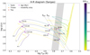 |
Fig. 6. Sargas’ position in the H-R diagram (best-fit from the β- and ω-models) together with selected evolutionary tracks from Georgy et al. (2013) at solar metallicity (Z = 0.014) for comparison. The selected tracks correspond (1) to initial masses enclosing Sargas’ mass, as indicated by the values (in M⊙) at the bottom-left (ZAMS position), and (2) to the two extreme rotation rates in Georgy’s et al. models, i.e., Ω = 0.95Ωc (multi-colored tracks) and Ω = 0 (yellow curves corresponding to evolution without rotation). The position of Sargas is represented by the three colored dots (connected by a dashed line) at the polar (Tp in blue), average ( |


From the measured  and estimated luminosity it seems that Sargas is located on the hot edge of the Cepheid instability strip. More striking, however, is the fact that the distinct Tp and Teq, resulting from GD, place Sargas’ polar regions outside the instability strip, while the equatorial are well inside it, as shown in Fig. 6 (check also the Teff maps in Figs. 2 and A.1). Based on this result, it would be interesting in the future to investigate the consequences of this partial location of Sargas on the Cepheid instability strip, notably concerning stellar pulsation.
Determining the age of a rapidly rotating star like Sargas is not a simple task since stellar evolution highly depends on the unknown initial rotation rate, in addition to classical quantities such as initial mass, mass loss, metallicity, overshooting, and also the dimensionality of the model (e.g., 1D, 2D, or 3D). In the framework of the grid of evolutionary tracks adopted here (with a rotation rate at ZAMS of ΩZAMS/Ωc = 0.95), and being conservative, we can roughly estimate Sargas’ age as ∼100 ± 15 Myr. For the adopted evolutionary tracks, this ΩZAMS/Ωc results in a rotation rate of ≃0.5 at Sargas’ age, which is lower than our measured value (≃0.85). This difference is not surprising since this rotation rate also depends on the quantities mentioned above as well as on the choice of model used, and in turn influences the estimated age. It is interesting to note that using identical models without rotation (ΩZAMS = 0 as shown in Fig. 6), Sargas’ age would be significantly underestimated (∼60%−70% of the estimated value).
6. Conclusions
In this work we used high-resolution interferometric (VLTI/PIONIER) and spectroscopic (VLT/UVES) data in order to measure several parameters of Sargas, an evolved fast rotator. We used the CHARRON code to compare the β- and ω-models of rotating stars (described in Sect. 3), which adopt the Roche approximation and include the important effects of GD and flattening. From a model-fitting procedure using an MCMC method, we measured several of Sargas’ physical parameters, namely Req, M, Veq, i, PArot, and  , as well as β, which is required in the β-model to describe the GD effect.
We showed that both models provide an equivalent description of Sargas, reproducing the observations equally well. This result agrees with those obtained in previous similar works on other fast rotators, and at the same time expands this agreement into a new region of the H-R diagram, never explored in this context of fast-rotation effects: the region of F-type bright giants/supergiants. Indeed, our results validate the ω-model for such stellar types, which is an important step forward in our understanding of stellar rotation effects because, as also discussed by Espinosa Lara & Rieutord (2011), this model provides a more physically profound comprehension of GD, without the need for the additional ad hoc β exponent required in the β-model.
Thanks to the measured physical parameters of Sargas we can provide a new, more precise, estimate of its spectral type. We can also guess its evolutionary status by placing it on theoretical evolutionary tracks of the H-R diagram given by the Geneva group (Georgy et al. 2013) for rotating stars. This allowed us to estimate Sargas’ age and show that it is probably located in the Hertzsprung gap, in the thin-shell-burning phase, just after reaching the Schönberg–Chandrasekhar limit. We have also shown that Sargas is placed very close to the hot edge of the Cepheid instability strip and, because of GD, its equatorial regions are inside this strip, while its polar regions are outside it.
All these intriguing and rare characteristics make Sargas a key target to understand the physics and the evolution of fast rotators of intermediate mass. Although 1D models provide a good starting point, a more profound comprehension of such rapidly rotating stars requires at least a 2D description of their physical structure and evolution. Such a star is obviously a strong motivation to develop 2D stellar models that can follow stellar evolution beyond the main sequence. This is precisely the new challenge of ESTER models (e.g., Espinosa Lara & Rieutord 2013; Rieutord et al. 2016; Gagnier et al. 2018).
Approved by the IAU-Working Group on Star Names (WGSN).
Jean-Marie Mariotti Center.
Code for High Angular Resolution of Rotating Objects in Nature.
Acknowledgments
This research has made use of the Jean-Marie Mariotti Center (JMMC) services OiDB (http://oidb.jmmc.fr), OIFits Explo-rer (http://www.jmmc.fr/oifitsexplorer_page.htm), LITpro (http://www.jmmc.fr/litpro), and GetStar (http://www.jmmc.fr/getstar), co-developed by CRAL, IPAG, and Lagrange/OCA. We are grateful to P. de Laverny for providing us the synthetic MARCS spectra from the AMBRE project. We also thanks D. R. Reese for his careful reading of the text and suggestions to improve it, and the referee (C. Haniff) for his critical and constructive remarks. Based on data obtained from the ESO Science Archive Facility under request number 257739. This research made use of the SIMBAD and VIZIER databases (CDS, Strasbourg, France) and NASA’s Astrophysics Data System. The authors also acknowledge the strong support of the French Agence Nationale de la Recherche (ANR), under grant ESRR (ANR-16-CE31-0007-01), which made this work possible. F. Espinosa Lara acknowledges the financial support of the Spanish MINECO under project ESP2017-88436-R.
References
- Adibekyan, V. Z., Benamati, L., Santos, N. C., et al. 2015, MNRAS, 450, 1900 [NASA ADS] [CrossRef] [Google Scholar]
- Anderson, E., & Francis, C. 2012, Astron. Lett., 38, 331 [NASA ADS] [CrossRef] [Google Scholar]
- Aufdenberg, J. P., Mérand, A., Coudé du Foresto, V., et al. 2006, ApJ, 645, 664 [NASA ADS] [CrossRef] [Google Scholar]
- Ayres, T. R. 2018, ApJ, 854, 95 [NASA ADS] [CrossRef] [Google Scholar]
- Castelli, F., & Kurucz, R. L. 2004, ArXiv e-prints [arXiv:astro-ph/0405087]. [Google Scholar]
- Che, X., Monnier, J. D., Zhao, M., et al. 2011, ApJ, 732, 68 [NASA ADS] [CrossRef] [Google Scholar]
- Chelli, A., Duvert, G., Bourgàs, L., et al. 2016, A&A, 589, A112 [NASA ADS] [CrossRef] [EDP Sciences] [Google Scholar]
- Claret, A. 2000, A&A, 363, 1081 [NASA ADS] [Google Scholar]
- Claret, A. 2017, A&A, 600, A30 [NASA ADS] [CrossRef] [EDP Sciences] [Google Scholar]
- Cotton, D. V., Bailey, J., Kedziora-Chudczer, L., et al. 2016, MNRAS, 455, 1607 [NASA ADS] [CrossRef] [Google Scholar]
- Cotton, D. V., Bailey, J., Howarth, I. D., et al. 2017, Nat. Astron., 1, 690 [NASA ADS] [CrossRef] [Google Scholar]
- Davis, J., Tango, W. J., & Booth, A. J. 2000, MNRAS, 318, 387 [NASA ADS] [CrossRef] [Google Scholar]
- de Jager, C., & Nieuwenhuijzen, H. 1987, A&A, 177, 217 [NASA ADS] [Google Scholar]
- de Laverny, P., Recio-Blanco, A., Worley, C. C., & Plez, B. 2012, A&A, 544, A126 [NASA ADS] [CrossRef] [EDP Sciences] [Google Scholar]
- de Laverny, P., Recio-Blanco, A., Worley, C. C., et al. 2013, The Messenger, 153, 18 [NASA ADS] [Google Scholar]
- Domiciano de Souza, A. 2014, Habilitation Thesis, Université Côte d’Azur (CNRS, Laboratoire Lagrange, France: Observatoire de la Côte d’Azur) [Google Scholar]
- Domiciano de Souza, A., Vakili, F., Jankov, S., Janot-Pacheco, E., & Abe, L. 2002, A&A, 393, 345 [NASA ADS] [CrossRef] [EDP Sciences] [Google Scholar]
- Domiciano de Souza, A., Kervella, P., Jankov, S., et al. 2003, A&A, 407, L47 [NASA ADS] [CrossRef] [EDP Sciences] [Google Scholar]
- Domiciano de Souza, A., Kervella, P., Jankov, S., et al. 2005, A&A, 442, 567 [NASA ADS] [CrossRef] [EDP Sciences] [Google Scholar]
- Domiciano de Souza, A., Zorec, J., & Vakili, F. 2012, in SF2A-2012: Proceedings of the Annual meeting of the French Society of Astronomy and Astrophysics, eds. S. Boissier, P. de Laverny, N. Nardetto, et al., 321 [Google Scholar]
- Domiciano de Souza, A., Kervella, P., Moser Faes, D., et al. 2014, A&A, 569, A10 [NASA ADS] [CrossRef] [EDP Sciences] [Google Scholar]
- Eggleton, P. P., & Tokovinin, A. A. 2008, MNRAS, 389, 869 [NASA ADS] [CrossRef] [Google Scholar]
- Espinosa Lara, F., & Rieutord, M. 2011, A&A, 533, A43 [NASA ADS] [CrossRef] [EDP Sciences] [Google Scholar]
- Espinosa Lara, F., & Rieutord, M. 2013, A&A, 522, A35 [NASA ADS] [CrossRef] [EDP Sciences] [Google Scholar]
- Foreman-Mackey, D., Hogg, D. W., Lang, D., & Goodman, J. 2013, PASP, 125, 306 [CrossRef] [Google Scholar]
- Gagnier, D., Rieutord, M., Charbonnel, C., Putigny, B., & Espinosa Lara, F. 2018, A&A, submitted [Google Scholar]
- Georgy, C., Ekström, S., Granada, A., et al. 2013, A&A, 553, A24 [NASA ADS] [CrossRef] [EDP Sciences] [Google Scholar]
- Glebocki, R., & Gnacinski, P. 2005, in 13th Cambridge Workshop on Cool Stars, Stellar Systems and the Sun, eds. F. Favata, G. A. J. Hussain, & B. Battrick, ESA SP, 560, 571 [Google Scholar]
- Goodman, J., & Weare, J. 2010, Commun. Appl. Math. Comput. Sci., 5, 65 [Google Scholar]
- Gray, R. O., & Garrison, R. F. 1989, ApJS, 69, 301 [NASA ADS] [CrossRef] [Google Scholar]
- Gustafsson, B., Edvardsson, B., Eriksson, K., et al. 2008, A&A, 486, 951 [NASA ADS] [CrossRef] [EDP Sciences] [Google Scholar]
- Haguenauer, P., Alonso, J., Bourget, P., et al. 2010, Proc. SPIE, 7734, 773404 [CrossRef] [Google Scholar]
- Hinkel, N. R., Timmes, F. X., Young, P. A., Pagano, M. D., & Turnbull, M. C. 2014, AJ, 148, 54 [NASA ADS] [CrossRef] [Google Scholar]
- Hoffleit, D., & Jaschek, C. 1991, The Bright Star Catalogue, 5th edn. (New Haven, CT: Yale Univ. Observatory) [Google Scholar]
- Hohle, M. M., Neuhäuser, R., & Schutz, B. F. 2010, Astron. Nachr., 331, 349 [NASA ADS] [CrossRef] [Google Scholar]
- Kervella, P., & Domiciano de Souza, A. 2006, A&A, 453, 1059 [NASA ADS] [CrossRef] [EDP Sciences] [Google Scholar]
- Kopal, Z. 1987, Ap&SS, 133, 157 [NASA ADS] [CrossRef] [Google Scholar]
- Le Bouquin, J.-B., Berger, J.-P., Lazareff, B., et al. 2011, A&A, 535, A67 [NASA ADS] [CrossRef] [EDP Sciences] [Google Scholar]
- Lucy, L. B. 1967, Z. Astrophys., 65, 89 [Google Scholar]
- McAlister, H. A., ten Brummelaar, T. A., Gies, D. R., et al. 2005, ApJ, 628, 439 [NASA ADS] [CrossRef] [Google Scholar]
- Monnier, J. D., Zhao, M., Pedretti, E., et al. 2007, Science, 317, 342 [NASA ADS] [CrossRef] [PubMed] [Google Scholar]
- Monnier, J. D., Che, X., Zhao, M., et al. 2012, ApJ, 761, L3 [NASA ADS] [CrossRef] [Google Scholar]
- Ochsenbein, F., & Halbwachs, J. L. 1982, A&AS, 47, 523 [NASA ADS] [Google Scholar]
- Ochsenbein, F., & Halbwachs, J. L. 1987, Bull. Inf. Centre Données Stellaires, 32, 83 [NASA ADS] [Google Scholar]
- Peterson, D. M., Hummel, C. A., Pauls, T. A., et al. 2006a, ApJ, 636, 1087 [NASA ADS] [CrossRef] [Google Scholar]
- Peterson, D. M., Hummel, C. A., Pauls, T. A., et al. 2006b, Nature, 440, 896 [NASA ADS] [CrossRef] [PubMed] [Google Scholar]
- Rieutord, M. 2016, in Lect. Notes Phys., eds. J.-P. Rozelot, & C. Neiner, (Berlin: Springer Verlag), 914, 101 [NASA ADS] [CrossRef] [Google Scholar]
- Rieutord, M., Espinosa Lara, F., & Putigny, B.2016, J. Comput. Phys., 318, 277 [NASA ADS] [CrossRef] [Google Scholar]
- Samedov, Z. A. 1988, Astrophysics, 28, 335 [NASA ADS] [CrossRef] [Google Scholar]
- Schönberg, M., & Chandrasekhar, S. 1942, ApJ, 96, 161 [NASA ADS] [CrossRef] [Google Scholar]
- See, T. J. J. 1896, Astron. Nachr., 142, 43 [NASA ADS] [CrossRef] [Google Scholar]
- Snow, T. P., Lamers, H. J. G. L. M., Lindholm, D. M., & Odell, A. P. 1994, ApJS, 95, 163 [NASA ADS] [CrossRef] [Google Scholar]
- Tallon-Bosc, I., Tallon, M., Thiébaut, E., et al. 2008, Proc. SPIE, 7013, 70131J [NASA ADS] [CrossRef] [Google Scholar]
- Tammann, G. A., Sandage, A., & Reindl, B. 2003, A&A, 404, 423 [NASA ADS] [CrossRef] [EDP Sciences] [Google Scholar]
- van Belle, G. T. 2012, A&ARv, 20, 51 [NASA ADS] [CrossRef] [Google Scholar]
- van Belle, G. T., Ciardi, D. R., Thompson, R. R., Akeson, R. L., & Lada, E. A. 2001, ApJ, 559, 1155 [NASA ADS] [CrossRef] [MathSciNet] [Google Scholar]
- van Belle, G. T., Ciardi, D. R., ten Brummelaar, T., et al. 2006, ApJ, 637, 494 [NASA ADS] [CrossRef] [Google Scholar]
- von Zeipel, H. 1924, MNRAS, 84, 665 [NASA ADS] [CrossRef] [Google Scholar]
- Zhao, M., Monnier, J. D., Pedretti, E., et al. 2009, ApJ, 701, 209 [NASA ADS] [CrossRef] [Google Scholar]
Appendix A: emcee fit results for the ω-model
 |
Fig. A.1. As in Fig. 2, but for the comparison of the interferometric observables of PIONIER with the ω-best-fit model (Table 2). |
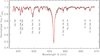 |
Fig. A.2. As in Fig. 3, but for the ω-model. We did not include here the β = 0 (fixed Teff) spectra since this parameter does not exist in the ω-model. Most of the important spectral lines are well reproduced by our best-fit model. |
Appendix B: Bandwidth smearing
When analyzing low-spectral-resolution (Rspec = λ/Δλ) interferometric data it is important to check the possible influence of the bandwidth-smearing effect in the corresponding observables. This effect arises from the fact that a finite (broad band) spectral bin contains interferometric information from different spatial frequencies. According to Davis et al. (2000), bandwidth smearing is negligible if
 (B. 1)
where ⌀ is the typical target’s angular size and  is the maximum projected baseline. In the case of PIONIER observations of Sargas considered in this work we have ξ ∼ 0.1, suggesting that the bandwidth smearing effect has a weak influence on the interferometric observables.
To more firmly confirm this, we computed a model adopting the parameters of our best-fit β-model (see Sect. 4), where the bandwidth smearing effect was included by sub-dividing the PIONIER spectral bins into 25 sub-channels. The interferometric observables computed for each sub-channel were then integrated over the wavelength range of the corresponding PIONIER spectral bin, resulting in observables that include bandwidth smearing and that can be directly compared to the data. This procedure allowed us to confirm that the difference between interferometric observables computed with and without bandwidth smearing are indeed negligible. In particular, the reduced χ2 are compatible within ≲0.1%.
The bandwidth smearing effect can therefore be ignored in the present work, which is a great advantage because computing the interferometric observables on a much larger number of wavelengths would be highly time consuming.
All Tables
All Figures
|
Fig. 1. uv coverage (units of spatial frequency) of VLTI/PIONIER observations of Sargas. The VLTI baselines used are identified with different colors (the corresponding AT stations are indicated in the upper legend). The six points per baseline correspond to the six spectral channels of the PIONIER H band observations as described in Sect. 2.1. Projected baselines Bproj range from ∼9 to ∼132 m. A zoom of the central region is shown in the right panel, corresponding to a maximum Bproj of ∼50 m. Image adapted from the OIFits Explorer service from JMMC. |
| In the text | |
|
Fig. 2. Comparison between interferometric observables from PIONIER (black dots with error bars) and from the β-best-fit model (red squares) presented in Table 2: squared visibilities V2 as a function of both spatial frequencies and baseline position angles (PA), and closure phases as a function of spatial frequencies defined at the longest baseline of the corresponding triangle. The error-normalized residuals of these comparisons are also shown (black dots); horizontal lines indicate the 0 (dashed line) and ±3σ (dotted line) reference values. The vertical dashed lines in the plots with PA abscissas indicate the PAs of the sky-projected rotation axis for the visible (PArot) and hidden (PArot − 180°) stellar poles. The two images at the bottom right show one specific intensity map, computed at the 1.62 μm spectral channel of the PIONIER data, and the Teff map corresponding to this β-best-fit model. These images are not rotated by PArot, i.e., they do not represent the star in sky coordinates. |
| In the text | |
|
Fig. 3. Comparison between the normalized flux from UVES (black dots with error bars) and from the β-best-fit model (red curve) presented in Table 2. The spectra shown span ∼26 nm centered on the Hα line, where the main atoms and ions contributing to the strongest absorption lines have been identified. These observations correspond to 257 selected wavelengths, which homogeneously sample the whole relevant spectral range, as shown by the data points. The thin curves correspond to normalized model fluxes for the same β-best-fit model, but where we have fixed Teff to Tp (blue) and Teq (green) over the whole photosphere (model without GD, i.e., β = 0). Clearly the complete best-fit model, with GD, better reproduces the observed spectral lines compared to the simpler model spectra computed with β = 0. |
| In the text | |
|
Fig. 4. Results obtained from the fit of the β-model to the interferometric and spectroscopic observations Sargas using the CHARRON and emcee codes (further details in the text). The figure shows one- (histograms) and two-dimensional projections of the posterior probability distributions obtained from the fitted parameters. The median (dashed lines) and uncertainties (dotted lines) obtained from the histograms for each fitted parameter are also indicated over the plots and correspond to the values given in Table 2. In the two-dimensional plots lower (higher) χ2 values correspond to darker (lighter) symbols; these 6000 points correspond to the converged final results of the MCMC model-fitting with emcee. |
| In the text | |
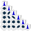 |
Fig. 5. As in Fig. 4 but for the ω-model. |
| In the text | |
|
Fig. 6. Sargas’ position in the H-R diagram (best-fit from the β- and ω-models) together with selected evolutionary tracks from Georgy et al. (2013) at solar metallicity (Z = 0.014) for comparison. The selected tracks correspond (1) to initial masses enclosing Sargas’ mass, as indicated by the values (in M⊙) at the bottom-left (ZAMS position), and (2) to the two extreme rotation rates in Georgy’s et al. models, i.e., Ω = 0.95Ωc (multi-colored tracks) and Ω = 0 (yellow curves corresponding to evolution without rotation). The position of Sargas is represented by the three colored dots (connected by a dashed line) at the polar (Tp in blue), average ( |
| In the text | |
|
Fig. A.1. As in Fig. 2, but for the comparison of the interferometric observables of PIONIER with the ω-best-fit model (Table 2). |
| In the text | |
|
Fig. A.2. As in Fig. 3, but for the ω-model. We did not include here the β = 0 (fixed Teff) spectra since this parameter does not exist in the ω-model. Most of the important spectral lines are well reproduced by our best-fit model. |
| In the text | |
Current usage metrics show cumulative count of Article Views (full-text article views including HTML views, PDF and ePub downloads, according to the available data) and Abstracts Views on Vision4Press platform.
Data correspond to usage on the plateform after 2015. The current usage metrics is available 48-96 hours after online publication and is updated daily on week days.
Initial download of the metrics may take a while.