| Issue |
A&A
Volume 619, November 2018
|
|
|---|---|---|
| Article Number | A3 | |
| Number of page(s) | 18 | |
| Section | Planets and planetary systems | |
| DOI | https://doi.org/10.1051/0004-6361/201832986 | |
| Published online | 30 October 2018 | |
Diagnosing aerosols in extrasolar giant planets with cross-correlation function of water bands
1
Observatoire astronomique de l'Université de Genève, Université de Genève,
51 chemin des Maillettes,
1290
Versoix,
Switzerland
e-mail: This email address is being protected from spambots. You need JavaScript enabled to view it.
2
Dipartimento di Fisica e Astronomia “Galileo Galilei”, Université di Padova,
Vicolo dell'Osservatorio 3,
Padova
35122,
Italy
3
Department of Physics, University of Warwick,
Coventry CV4 7AL,
UK
4
Center for Space and Habitability, University of Bern,
Sidlerstrasse 5,
3012,
Bern,
Switzerland
5
INAF – Osservatorio Astronomico di Padova,
vicolo dell’Osservatorio 5,
35122,
Padova,
Italy
Received:
9
March
2018
Accepted:
16
July
2018
Abstract
Transmission spectroscopy with ground-based, high-resolution instruments provides key insight into the composition of exoplanetary atmospheres. Molecules such as water and carbon monoxide have been unambiguously identified in hot gas giants through cross-correlation techniques. A maximum in the cross-correlation function (CCF) is found when the molecular absorption lines in a binary mask or model template match those contained in the planet. Here, we demonstrate how the CCF method can be used to diagnose broadband spectroscopic features such as scattering by aerosols in high-resolution transit spectra. The idea consists in exploiting the presence of multiple water bands from the optical to the near-infrared. We have produced a set of models of a typical hot Jupiter spanning various conditions of temperature and aerosol coverage. We demonstrate that comparing the CCFs of individual water bands for the models constrains the presence and the properties of the aerosol layers. The contrast difference between the CCFs of two bands can reach ~100 ppm, which could be readily detectable with current or upcoming high-resolution stabilized spectrographs spanning a wide spectral range, such as ESPRESSO, CARMENES, HARPS-N+GIANO, HARPS+NIRPS, SPIRou, or CRIRES+.
Key words: planets and satellites: atmospheres / planets and satellites: composition / techniques: spectroscopic
© ESO 2018
1 Introduction
High-resolution (R ~ 105), ground-based transmission spectroscopy offers a unique insight into exoplanetary atmospheres. At such high-resolution, (1) telluric contamination, which dramatically hampers lower resolution, ground-based observations (Sing et al. 2015; Gibson et al. 2017) is better removed (Astudillo-Defru & Rojo 2013; Allart et al. 2017); (2) the resolved cores of the alkali atoms sound up to the base of the thermosphere (P ≲ 10−9 bar; Wyttenbach et al. 2015, 2017); (3) individual absorption lines of molecular bands are spectrally resolved and chemical species, such as H2O and CO, are uniquely identified (Snellen et al. 2010; de Kok et al. 2014; Brogi et al. 2018).
Single molecular bands have been detected with high-resolution transmission spectroscopy in the near-infrared (NIR) by exploiting cross-correlation techniques (e.g. Brogi et al. 2016). Hoeijmakers et al. (2015), Allart et al. (2017), and Esteves et al. (2017), have proposed an extension of this method to the optical bands. However, optical to NIR high-resolution spectrographs are only available from the ground1, thus the effectiveness of these techniques has been limited by the presence of Earth atmosphere.
One aspect of the problem is that high-resolution transmission spectroscopy requires a normalization of the flux of the spectra acquired during the night, that can vary due to air mass or instrumental effects (Snellen et al. 2008; Wyttenbach et al. 2015, 2017; Heng et al. 2015). During the process, the absolute level of the absorption of the planet is lost, and broadband features such as those due to aerosols could be removed from the spectra. Indeed, the presence of aerosols on exoplanets was inferred with space-borne Hubble Space Telescope (HST) observations (e.g. Charbonneau et al. 2002; Ehrenreich et al. 2014; Kreidberg et al. 2014a; Wakeford et al. 2017, but see also Snellen 2004; Di Gloria et al. 2015) or lower resolution spectrophotometric observations (e.g. Bean et al. 2010; Nascimbeni et al. 2013; Lendl et al. 2016), revealing that they are very common on hot Jupiters (Sing et al. 2016; Barstow et al. 2017) and smaller Saturn- and Neptune-size planets. Brogi et al. (2017), who did not treat the effect of aerosols explicitly, and Pino et al. (2018) demonstrated that a combined analysis of ground-based, high-resolution and space-borne, low- to medium-resolution transmission spectra can better constrain the chemical and physical conditions of exoplanetary atmospheres.
Single spectral features such as the sodium doublet can be used to infer the presence of aerosols (Charbonneau et al. 2002; Snellen et al. 2008; Heng 2016; Wyttenbach et al. 2017). Here we demonstrate quantitatively that high-resolution transmission spectroscopy of molecular bands can be used to distinguish between aerosol-free and aerosol-rich scenarios (as qualitativelynoted by de Kok et al. 2014). The technique exploits the fact that the opacities of water vapour and aerosols behave differently with wavelength: the former increases with wavelength, while the latter is usually constant or decreasing in the optical and NIR regions of the spectrum. The relative contrast of water bands can thus be used as a diagnostic of the presence of aerosols. At high resolution, the contrast of water bands can be measured through their cross-correlation functions (CCFs). This is obtained by cross-correlating each water band with a binary mask, and can thus be regarded as the average line profile within the band.
We usedthe πη code (Pino et al. 2018; see also Ehrenreich et al. 2006, 2012, 2014) to build a grid of models representative of a hot Jupiter in different temperature conditions, containing aerosols at different altitudes; built the CCFs of the grid with a set of binary masks representing water bands of interest (following the technique introduced by Allart et al. 2017); discuss how the relative contrast of different water absorption bands is an indicator of the cloudiness of an atmosphere.
Our technique is suitable for applications with the roster of current and next generation high-resolution (R ≳50 000), stabilized, optical-to-NIR Echelle spectrographs with extended spectral coverage (Δ λ ≳ 2000 Å). A non-comprehensive list includes HARPS + NIRPS, GIARPS (GIANO + HARPS-N), ESPRESSO, CARMENES, SPIRou, ARIES, IGRINS, IRD, HPF, iLocater, PEPSI, EXPRES, NEID (McCarthy et al. 1998; Mayor et al. 2003; Oliva et al. 2006; Pepe et al. 2010; Yuk et al. 2010; Cosentino et al. 2012; Thibault et al. 2012; Mahadevan et al. 2012; Quirrenbach et al. 2014; Kotani et al. 2014; Crepp et al. 2014; Strassmeier et al. 2015; Conod et al. 2016; Jurgenson et al. 2016; Schwab et al. 2016; Claudi et al. 2017). Of particular interest is the HIRES optical-to-NIR spectrograph for the E-ELT (Zerbi et al. 2014; Marconi et al. 2016), HROS (TMT Project 2013) for the TMT, and G-CLEF (Szentgyorgyi et al. 2012, 2014) for the GMT. At longer wavelengths (λ ≳ 2 μm), an extension of our technique is possible and warranted in view of future instruments such as CRIRES+ (Follert et al. 2014), METIS (Brandl et al. 2014), NIRES-R, and GMTNIRS. See Crossfield (2014) and Wright & Robertson (2017) for a description of most of these instruments.
2 Methods
First, we selected the relevant spectral bands. We considered two cases: without telluric contamination (ideal case) and with telluric contamination (realistic case). This yielded two sets of bands listed in Tables 1 and 2, respectively2 (see also Fig. 1). The ideal case informs on the potential of a high-resolution optical to NIR spectrograph mounted on a space-borne or stratospheric facility. While such an instrument will not be delivered within the next decade, similar concepts have already been developed (LUVOIR; France et al. 2017; HIRMES3; on-board SOFIA). On the other hand, from the ground, Allart et al. (2017) demonstrate how telluric lines can be efficiently corrected for in the optical. In the NIR, the contamination is more severe. Although telluric correction or self-calibration using time resolution and the measured flux variations (de Kok et al. 2013; Birkby et al. 2013) both work effectively for unsaturated telluric lines, portions of the spectrum completely saturated, for example at the centre of strong water lines, cannot be recovered. We thus selected regions where the features in the telluric transmittance spectrum, taken from Hinkle et al. (2003), remove less than 80% of the flux, and correction is possible. These bands roughly correspond to the windows of transparency of Earth atmosphere, and we named them accordingly (see Table 1, and orange regions in Fig. 1).
We computed the expected CCF contrast in each band, following three steps. Firstly, we simulated a theoretical template transmission spectrum of an exoplanet at R ~ 106; secondly, wesimulated observations of each water band with a relevant spectrograph (see Table 1), by convolving at the appropriate resolving power and binning to the instrumental resolution; thirdly, we computed the CCF with a binary mask.
In the following, we describe these three steps (see Pino et al. 2018 for a more detailed description of the routines used in the first two steps).
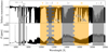 |
Fig. 1 Bands used to compute the CCF of water, on top of the telluric transmittance (upper panel), and an exoplanet transmission spectrum model (lower panel). Grey bands correspond to water vibrational band. Orange bands correspond to the windows of transparency of Earth atmosphere. The bands partially overlap, as indicated by toothed areas. Upper panel: the solid black line represents the transmittance of Earth atmosphere (Hinkle et al. 2003), ranging from 1 (all incident light transmitted) to 0 (all incident light absorbed). Besides water bands, corresponding to the bands in the bottom panel, molecular oxygen, carbon dioxide, and methane show the most prominent features. Lower panel: the solid black line represents a theoretical cloud-free isothermal model of HD189733b. Within each water vibrational band, the region of the spectrum in grey represents the spectrum seen through a selected instrument, thus convolved at the appropriate resolving power (see Table 1). |
Definition of the water absorption bands.
2.1 High-resolution template
We first used the πη 1D line-by-line radiative transfer code (Pino et al. 2018) to compute high-resolution model transmission spectra δ(λ) = 1 − fin∕fout, where fin∕out are the stellar fluxes registered in- and out-of-transit. A line-by-line approach is necessary to apply the CCF technique, as the molecular lines need to be singularly resolved. The water cross section used in the models was calculated from a high-resolution opacity table ( , R ~ 106). The table was obtained with the HELIOS-K routine applied to the HITEMP line-list (Grimm & Heng 2015), accurate up to the high temperatures expected in hot Jupiters (Teq ≳ 1000 K).
We assumed the planetary parameters of HD189733b, a typical hot Jupiter (rp=10 bar = 1.108 RJ, Mp = 1.138 MJ, R⋆ =0.756 R⊙). Besides water (volume mixing ratio, VMR = 10−3), we added opacities from sodium(VMR = 10−6), potassium (VMR = 10−7), and Rayleigh scattering and collision-induced absorption (CIA) by H2. Different parameters were varied to produce the templates:
- 1.
Aerosol altitude. For illustrating the technique, a simple parametrization of the aerosol deck is sufficient. We set the atmosphere to be opaque at all wavelengths for pressures higher than a threshold pc. In the spectral range considered (<2 μm), this parametrization simulates aerosol particles of size ≳2 m. We vary pc between 10 and 10−7 bar) in steps of 1 dex (i.e. equally spaced on a logarithmic scale).
- 2.
Temperature of the atmosphere. We assumed isothermal temperature–pressure (T–p) profiles, at first order adequate to describe water absorption in transmission spectra (Heng & Kitzmann 2017). Temperature is varied between 1200 and 2300 K in steps of ~200 K.
We show a set of templates built for a temperature of T = 1700 K in the upper panels of Figs. 6 and 9. Grey vertical bands correspond to the regions that we analysed in the idealized case and in the realistic case that avoids the peak of telluric contamination, respectively.
2.2 Convolution with the LSF and binning
When observed with a spectrograph, spectral lines are convolved with the instrumental line spread function (LSF). Even for high-resolution instruments such as HARPS(-N) or ESPRESSO planetary molecular lines are narrower than the instrumental LSF (~ 2–3 km s-1 wide). Indeed, the Doppler width for water lines at typical temperatures of a planetary atmosphere (500–3000 K) ranges between 0.7 and 1.5 km s-1. This convolution effect is strong for resolving powers <100 000, and needs to be taken into account when estimating the contrast of the CCF (see Fig. 2). We convolved lines in each water band with a Gaussian LSF representative of an instrument covering that wavelength range. For illustration, we chose to simulate observations with HARPS(-N), ESPRESSO, GIANO (see Tables 1 and 2), but the technique is applicable to any high-resolution spectrograph with enough spectral coverage (see Sect. 1).
Transmission spectra are built by dividing out stellar spectra taken during the transit and out-of-transit, which are thus individually convolved with the instrumental LSF. Pino et al. (2018) discuss how models should follow the same steps, since mathematically the order of division and LSF convolution cannot be interchanged (see also Deming & Sheppard 2017). In this paper, we assumed that the stellar host star has no water lines, a reasonable assumption for many cases (Brogi et al. 2016). Thus, the stellar spectrum on the background of planetary water absorption is on average flat, and the direct convolution of the planetary absorption and the instrumental LSF is possible.
As discussed in Pino et al. (2018), a key ingredient of realistic simulations is binning the model to the correct resolution, that is the step with which the spectrum is sampled. For the various bands, we adopted the resolution elements reported in Tables 1 and 2. For ESPRESSO, we assumed that the resolution element is the same as for HARPS(-N).
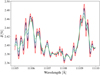 |
Fig. 2 Effect of finite resolving power on water lines. The red curve corresponds to a line-by-line model (with a resolution of R ~ 106). From the light green curve to the purple curve, we show the same spectrum convolved with Gaussian LSF corresponding to the following resolving powers: at R = 50 000 (GIANO), at R = 75 000 (similar to CARMENES), at R = 115 000 (HARPS/-N), and at R = 134 000 (ESPRESSO). At the lowest resolving power, the individual molecular lines are not entirely resolved. |
2.3 Cross-correlation
Individual molecular lines are weak and usually buried in the noise. However, we can enhance our detection capabilities by averaging the signal coming from hundreds or thousands of lines. This is achieved by building a cross-correlation function (CCF4; Baranne et al. 1979, 1996; Pepe et al. 2002). To compute the CCF, we followed the method developed by Allart et al. (2017) to search for water in the HARPS optical spectra of HD189733b. The cross-correlation function is defined as
![Mathematical equation: \begin{equation*}CCF_{N,\,T_{ll}}(v)=\frac{1}{N}\sum_{i=1}^N S(\lambda_i)\cdot M\left[\lambda_i \left(1 + \frac{v}{c} \right)\right]. \end{equation*}](/articles/aa/full_html/2018/11/aa32986-18/aa32986-18-eq2.png) (1)
(1)
A binary mask M (with an aperture of one pixel, i.e. 0.82 km s-1 in HARPS and ESPRESSO and 6.38 km s-1 in GIANO) is projected on the spectrum S. The binary mask corresponds to the theoretical wavelengths λi of the N lines of the molecule we are looking for, drawn from a line list at a temperature Tll. Doppler shifting the mask in the radial velocity (v) domain with steps of one pixel, c being the speed og light, allows one to reconstruct the shape of the average molecular line. Following Allart et al. (2017), we inspected the − 80∕+80 km s-1 range. Since no wavelength shift was introduced in the model, we expect a peak at 0 km s-1.
With reference to Eq. (1), S is one of the water bands defined in Table 1 (without considering telluric absorption) or Table 2 (considering it), convolved with the appropriate LSF and binned at the instrumental resolution. We built a dedicated mask for each water band starting from the HITEMP line list. Within the wavelength range of each water absorption band, we selected the 800 lines with strongest spectral line intensity at a temperature Tll = 1 200 K5, typical of the terminator region of hot Jupiters. We note that the choice of the mask is not unique. However, the specific choice we made does not impact the conclusions of the study6.
The CCF of a water absorption band is rich in information, as it encodes the average line profile within the band. In this work, we are only interested in the line contrast. We thus fit a Gaussian profile f(v) to our computed CCF of the form
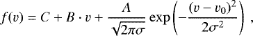 (2)
(2)
leaving C, B, A, σ, and v0 as free parameters. The contrast of the CCF (i.e. of the average line in the absorption band) is then 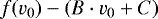 .
.
We show examples of simulated CCFs in Fig. 3, for the  and
and  bands, observed with ESPRESSO and GIANO, respectively. The different resolving power of the observations is clear from the different width of the CCFs. Furthermore, the sampling of the CCF is determined by the sampling of the instrument, which is higher for ESPRESSO (in order to oversample the narrower LSF). We stress that the contrast of the CCF is also dependent on the resolving power (since energy is conserved), and it is thus vital to know well the instrumental profile (hence the choice of stabilized spectrographs with oversampled LSFs). A red dashed line shows the fit to the case of pc = 0.01 mbar performed using Eq. 2. The fit is in good agreement with the simulations. Similar fits were performed for each simulated CCF (not shown).
Definition of the water absorption bands in the presence of telluric absorption.
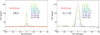 |
Fig. 3 CCFs for the |


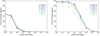 |
Fig. 4 Contrast of the CCF as a function of altitude of aerosols (expressed as pressure of the cloud top). Lighter colours indicate colder models, darker colours indicate hotter models (between 1200 and 2300 K), as indicated by the colour-matched labels. Left panel: |


3 Results and discussion
3.1 Ideal case
We first discuss the case of solar water abundance with an opaque, grey absorber found at a pressure pc, representing a population of particles of size ≳2 μm (see Sect. 2.1) in the ideal case (telluric absorption neglected). In Fig. 4, we showcase the contrast of the CCF for models at various temperatures as a function of pc for two example bands ( and
and  ). The following conclusions drawn from this example hold also for the other bands. Firstly, the CCF of the redder bands have a stronger contrast than the CCF of the bluer bands; secondly, the higher in the atmosphere the aerosols are found, the more damped is the signal. A sharp drop in the signal is observed for aerosols higher than a critical pressure; thirdly, the precise value of this critical pressure depends on which band is considered; finally, the temperature dependence, represented by curves of different colours in Fig. 4, is modest.
Within our grid, temperature varies by a factor of approximately two, but the CCF contrast in each band varies by less than 10% between the coldest (1200 K) and the hottest (2300 K) model. At first glance, it is surprising that the CCF contrast is not linearly increasing with temperature, since at first order the contrast of every atmospheric signature is proportional to temperature through the scale height. Indeed, the contrast of the sodium and potassium doublets nearly doubles between the hottest and the coldest temperatures considered (Fig. 5, left panel). However, in high-resolution transmission spectroscopy of molecules, the strongly non-linear relation between temperature and population of energetic levels plays an important role, by impacting the relative strength of single molecular lines (see right panel of Fig. 5). The net effect is that, for a hotter atmosphere, the gain in signal due to the increased scale height is partially lost. We emphasize that optimization of detection techniques of molecular signatures through cross-correlation needs to properly account for this factor (Allart et al. 2017).
Figure 6 shows the contrast of the CCF of all considered water bands in the ideal case. Here, each colour corresponds to a cloud deck at a given pressure, as shown in the upper panel. In the lower panel, the vertical error bar in each band represents the CCF contrast values spun when temperature is varied between 1200 and 2300 K. The fact that curves corresponding to different values of pc do not overlap means it is possible to discriminate among the different cases. The models are best distinguished with a broad wavelength coverage. We indicate as vertical error bars the 1-pixel 1σ precision of HARPS and ESPRESSO, obtained with the respective exposure time calculators (ETCs) and compatible with Allart et al. (2017), and valid for HD189733b. The CCF spans about 5 pixels (Allart et al. 2017), implying that the 1σ photon noise precision on the CCF is even better. However, additional noise is introduced by telluric residuals (see Appendix A). In particular, the technique can only be used for targets with a combination of systemic velocities and BERV such that telluric lines are moved by a few resolution elements; otherwise, telluric absorption would contaminate, or even hinder, the planetary signal. The NIR bands investigated in this section are not accessible from the ground for the presence of telluric absorption, and we did not attempt an estimation of the precision of a hypothetical space-borne or stratospheric high-resolution spectrograph (see Appendix A and Sect. 2). However, it is clear that a HARPS-like precision would suffice to detect the CCF of the NIR water bands at high confidence in the absence of telluric noise.
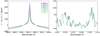 |
Fig. 5 Temperature dependence of the high-resolution transmission spectrum of a hot Jupiter. The temperature varies between 1200 and 2300 K in steps of ~200 K (from light to dark). Left panel: zoom on one line of the sodium doublet. The contrast of the sodium feature in the hottest atmosphere (purple) is approximately twice its contrast in the coldest atmosphere (light green). This behaviour is explained through the linear dependence of atmospheric signal on temperature through the scale height. Right panel: zoom on a region of the
|

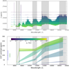 |
Fig. 6 Results in the ideal case. Upper panel: high-resolution models of a hot Jupiter with T = 1700 K and differentvalues of pc, ranging between 10−7 and 1 bar. Each colour corresponds to a different value of pc, and the lightest colours correspond to condensates deeper in the atmosphere. Lower panel: CCF contrast as a function of wavelength. The colours are in correspondence with the models shown in the upper panel. For each value of pc, the temperature range 1200–2300 K is explored. We indicate with a vertical error bar the induced variation in the contrast of the CCF. On the left, the 1-pixel, 1σ precision of HARPS (blue) and ESPRESSO (green) for a single transit are shown. These error bars only account for photon noise, but telluric residuals may introduce additional noise (see Appendix A). The NIR bands must be accessed from space or from the stratosphere. Such instruments do not yet exist, and we do not estimate an error bar. |
3.2 A metric to diagnose aerosols
The fact that the critical pressure above which the CCF is damped differs from band to band is crucial to discriminate aerosol-free and aerosol-rich atmospheres. This is quantified by the difference between the CCF contrast of pairs of bands (Δ C). In Fig. 7, we showcase this difference for the bands  and
and  . This difference is significantly higher when aerosols are found around 1–10 mbar, high enough to conceal the
  water band at 7200 Å but not the
  water band at 19 000 Å. The contrast difference ΔC between different pairs of bands peaks for different pressures of the aerosols, depending on the value of the critical pressure of both bands. Furthermore, the maximum value of ΔC indicates how much the pair of bands discriminates among models. We performed this analysis for every pair of bands, and show the results in Fig. 8. Overall, combinations of bands covering the optical to the NIR can discriminate at the 200 ppm level aerosol decks at 1 bar < pc < 0.1 mbar, and for the considered instruments.This value of ΔC is readily detectable with current or upcoming stabilized spectrographs in the optical, and with a space-borne or stratospheric NIR instrument of similar performance. Indeed, rescaling the precision obtained by Allart et al. (2017) to a CCF built with 800 lines yields a 1-pixel precision of 62 ppm on the CCF contrast with HARPS, and of 24 ppm with ESPRESSO in a single transit (see also Appendix A). We summarize in Table 3 the maximum value of ΔC and the pressure range where it is achieved for different pairs of water bands observed with HARPS-N, ESPRESSO and GIANO as detailed in Tables 1 and 2. Higher resolving power, especially in the NIR, would provide even higher values of ΔC.
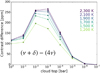 |
Fig. 7 Difference in contrast between the CCF of the |


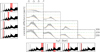 |
Fig. 8 Sensitivity of different combinations of water bands to the presence of aerosols. Each panel shows the difference between the band highlighted in the bottom row and the band highlighted in the left column. The x- and y-axes are the same as for Fig. 7, running between 1 and 10−7 bar and between 0 and 300 ppm, respectively. Orange and green horizontal dashed lines are put in correspondence to the 100 and 200 ppm levels. |
Typical CCF contrast difference (ΔC) between pairs of water bands and pressure range where this maximum difference is reached.
3.3 Telluric contamination
We repeated the analysis focusing on the infrared transparency windows of Earth. These coincide with the transparency windows in the exoplanet. In transmission geometry, the loss in absorption is not so abrupt because the stellar light-rays cross transversely the atmosphere. The net result is that the analysis is still sensitive to the presence of aerosols, but at the reduced level of ~ 100 ppm (see Table 4 and Fig. 10). This is likely already enough to detect the presence of aerosols with the simulated GIARPS and ESPRESSO observations (see Table A.1). This is demonstrated by adding to our simulated observations the impact of telluric absorption, as described in Appendix A. We accounted for both the increase in the photon noise due to the reduced photon count in the core of telluric water lines, and for residuals of an imperfect telluric correction.
Moreover, at least two strategies to further increase the signal are possible:
- 1.
We did not fully explore the wavelength range. CARMENES is sensitive to two other water bands not considered in this work, that are less intense but much less contaminated by telluric lines, thus likely accessible from the ground; GIANO is sensitive also to the K band, not considered here;
- 2.
We simulated GIANO observations in the NIR. GIANO has a resolving power of ~50 000, however instruments at higher resolving power are available (CARMENES) and several others will be in the near future (NIRPS, SPIRou, CRIRES+, etc.). A higher resolving power has the advantage that the CCF contrast is higher, because of the narrower LSF and because less molecular lines are blended in the spectrum (see Fig. 2).
Typical CCF contrast difference (ΔC) between pairs of water bands and pressure range where this maximum difference is reached when considering regions where telluric correction is possible.
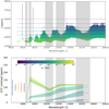 |
Fig. 9 CCF contrast as a function of wavelength in the case where telluric contamination is considered, in the presence of a grey opacity source simulating large condensates at various pressure levels. Upper panel: high-resolution models of a hot Jupiter with T = 1700 K. Each colour corresponds to a different value of pc, ranging between 10−7 and 1 bar, and the lightest colours correspond to condensates deeper in the atmosphere. Lower panel: CCF contrast as a function of wavelength. The colours are in correspondence with the models shown in the upper panel. For each value of pc, the temperature range 1200–2300 K is explored. We indicate with a vertical error bar the induced variation in the contrast of the CCF. On the left, the 1σ precision of HARPS (blue), ESPRESSO (green), GIANO (orange, red, and black) for the Y, J, and H bands for a single transit are shown. These error bars only account for photon noise, but telluric residuals may introduce additional noise (see Appendix A). |
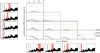 |
Fig. 10 Sensitivity to the presence of aerosols of different combinations of bands that are accessible from the ground even in the presence of tellurics. Each panel shows the difference between the band highlighted in the bottom row and the band highlighted in the left column. The x- and y-axes are the same as for Fig. 7, running between 1 and 10−7 bar and between 0 and 300 ppm, respectively. Orange and green horizontal dashed lines are put in correspondence to the 100 and 200 ppm levels. We note that these values are arbitrary. Scatterers up to the 0.1 mbar level produce values of ΔC up to 100 ppm. |
3.4 Non-grey aerosols
The assumption that aerosols have a grey scattering cross-section is only valid for particles of size larger than about 2 μm, and up to λ~ 3 μm. We discuss the more general scenario of non-grey aerosols, without performing full simulations that would require an implementation of the Mie theory of scattering.
At wavelengths longer than 3 μm, distinctive absorption features of aerosols species such as water or silicates become prominent in transmission spectra (de Mooij et al. 2013; Mollière et al. 2017). These relatively narrow features uniquely identify the compositionof aerosols, making them probes of the chemistry of exoplanets. However, at wavelengths longer than 5 μm, where the majority of such features are located, the sky background is too bright for ground-based spectrographs to be effective (Snellen et al. 2013).
In the wavelength range <2 μm that we considered in this paper, the Rayleigh limit of Mie scattering from “small” particles with sizes typically smaller than about 1 μm results in a cross section of aerosols that decreases with wavelength with a typical slope, if they are present (e.g. Pinhas &Madhusudhan 2017; the precise particle size depends also on the wavelength of incident light and is smaller in the optical). Several hot Jupiters host aerosols of this kind (Sing et al. 2016; Barstow et al. 2017). Compared to the grey aerosols considered heretofore, this scenario exacerbates the difference in contrast between the optical water bands, even more affected by scattering from this kind of aerosols, and the NIR water bands. Δ C is thus increased, and aerosols are readily detected also in this case. We tested this by simulating an atmosphere compatible with HD189733b, which hosts a marked optical slope attributed to this kind of particles (Pont et al. 2013; Pino et al. 2018). In this case Δ C reaches up to 100 ppm, and aerosolsare thus promptly detected.
The chromatic dependence of the cross section of small aerosols makes it more challenging to locate their height in the atmosphere.Yet, its slope and uniformity indicate the distribution of the sizes of the scattering particles and their composition (Berta et al. 2012; Pont et al. 2013; Wakeford & Sing 2015; Pinhas & Madhusudhan 2017). An extension of the technique that we presented has thus the potential to characterize the population of aerosols in the atmosphere. However, a detailed assessment requires detailed modelling of Mie scattering by aerosols, and is out of the scope of this paper.
Snellen (2004), Di Gloria et al. (2015), and Heng (2016) presented alternative techniques that are able to constrain the presence of chromatic scattering by aerosols through high-resolution spectrographs of the kind we considered. If chromatic scattering can be excluded using such techniques, Δ C can be used to infer the altitude of aerosols as discussed in Sect. 3.2.
3.5 Water abundance
Throughout the paper we have assumed a solar VMR for water. This is broadly supported by equilibrium chemistry calculations over a broad range of temperatures (e.g. Sharp & Burrows 2007; Miguel & Kaltenegger 2014) and by current observational evidence (e.g. Crossfield 2015; Todorov et al. 2016). However, determining the absolute abundance of water from observations is challenging (see, e.g., Kreidberg et al. 2014b; Wakeford et al. 2018). We first discuss the observational strategy to measure the water mixing ratio in transmission and its limitations. Then, we show that an uncertainty in the VMR of water directly translates in an uncertainty in the altitude of aerosols inferred under the assumption of a grey aerosol deck (see Sect. 3.2). A similar impact on the inferred properties of aerosols (particle size distribution, composition, etc.) is expected in the more general case of chromatic scattering by aerosols (see Sect. 3.4).
Measuring the VMR of atomic and molecular species with ground-based, high-resolution transmission spectroscopy. High-resolution spectra from the ground can only provide measurements of the difference between the transit depths at different wavelengths. We now consider two atomic/molecular atmospheric species 1 and 2, that are the dominating source of opacity at wavelengths λ1 and λ2, respectively.Lecavelier Des Etangs et al. (2008) and Désert et al. (2009) first have shown how to relate the difference between the transit depths at these two wavelengths to the abundance ratio of the atmospheric species. The same result can be obtained by using Eq. (12) by Heng & Kitzmann (2017), valid in the isothermal, isobaric case. Indeed, by dividing by the stellar radius and differentiating this equation, the difference in the transit depth at the two wavelengths can be related to the volume mixing ratio and the cross section of the dominating spectral feature at the two wavelengths as
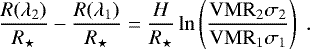 (3)
(3)
The scale height H can be inferred by comparing the observed planet radius at different wavelengths where the cross-section is known (Benneke & Seager 2012). At high resolution, this is possible by using multiple bands of the same molecule where aerosols have a small impact. Unfortunately, water is not well suited to the task from the ground, since the contrast of the CCF in the Y, J and H transparency windows is impacted by relatively low aerosols at the 10−1 bar level. Other molecules such as methane and titanium monoxide, or atomic species such as the alkali doublets (Heng 2016), may be better suited, since they are less impacted by telluric absorption.
Without tellurics contamination, for example from a hypothetical space-borne or stratospheric high-resolution spectrograph, the water bands  and
and  are ideally suited. Indeed, by rearranging Eq. (3) and evaluating it in the
  and
and  water bands, we can isolate the scale height:
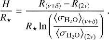 (4)
(4)
From Fig. 8, we see that the contrast difference between the two bands is constant for aerosols up to 10−4 bar. In this region, the contrast difference is set by the intrinsic difference in contrast between the bands, and is thus a probe of scale height. Farther in the infrared, stronger molecular bands may be even better suited for the task.
Besides knowing the scale height, a second step is necessary to measure the volume mixing ratio VMR2 of a given constituent using Eq. (3). Indeed, we need to compare the transit depth in a wavelength region where it is the dominating source of opacity to a region where the dominating source of opacity has a known VMR1. Then, we can invert Eq. (3) to get VMR2.
Measuring the VMR of atomic and molecular species with space-borne spectroscopy, photometry, or multi-object spectroscopy. The operations described in the previous paragraph can be performed without directly measuring the transit depth but only comparing excesses in different bands. They are thus possible with ground-based high-resolution facilities. Yet, an hypothetical space-borne or stratospheric high-resolution spectrograph may be able to directly measure the transit depth, as the effect of Earth atmosphere is absent or severely limited. Already now, the transit depth can be measured from space, or with photometric and multi-object spectroscopic techniques from the ground, albeit at lower resolution (up to R ~ 103, too low to apply the CCF technique).
However, even a direct measurement of the transit depth within a molecular band is not sufficient to infer its VMR. Indeed, the pressure-radius7 pref (rref) at an arbitraryreference level must be known. This can be obtained by directly measuring the transit depth in an absorption feature generated by a species of known VMR (Lecavelier Des Etangs et al. 2008).
Lecavelier Des Etangs et al. (2008) proposed Rayleigh scattering by H2 as such a comparison feature. However, the task of detecting the absorption feature of molecular hydrogen is hindered in the presence of Rayleigh scattering by aerosols that may contaminate the optical region of the spectrum. As discussed in Sect. (3.4) measuring the slope of the optical transmission spectrum and its uniformity provides hints on whether aerosols of small size are present or not in the atmosphere.
Effect of an uncertain water VMR. It is thus worth getting an idea of the effect of an uncertain water abundance on our conclusions. Analytical formulas provide a first insight. Lecavelier Des Etangs et al. (2008) define the equivalent altitude zeq by the altitude in the atmosphere such that a sharp occulting disk of radius equal to the sum of the planetary radius and zeq produces the same absorption depth as the planet and its translucent atmosphere. We can reformulate the concept as an equivalent pressure peq by
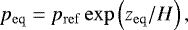 (5)
(5)
where pref is the pressure at the arbitrarily chosen reference level. Within a water band n, water is the dominant source of opacity, thus we can write
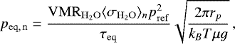 (6)
(6)
where  is the average cross section of the water lines within the nth molecular band, τeq ~ 0.56 is the equivalent optical depth (Lecavelier Des Etangs et al. 2008), T is the atmospheric temperature, μ is the mean molecular weight of the atmospheric constituents, and g is the surface gravity.
At first order, to determine if a water band is occulted or not by aerosols, we can compare its equivalent pressure with the pressure where aerosols are located. Thus, the drop in the contrast of the CCF shown in Fig. 4 is located around the equivalent pressure within the considered water band.
To qualitatively understand the effect of the variation of  , it is sufficient to note that, from Eq. (6), it follows that
 (7)
(7)
where peq, n, ⊙ is the equivalent pressure when water is present in the atmosphere at solar abundance.
We tested numerically our intuition, by repeating the full analysis with  (about 0.1 the solar value). In Fig. 11 we compare the contrast of the CCF of the
  band for
  (blue) and
  (red). When
  is decreased by a factor of 10, aerosols located at pressures of a factor of 10 higher, thus deeper in the atmosphere, are sufficient to occult the water band, confirming Eq. (7).
The conclusion that high-resolution transmission spectroscopy of water over a broad wavelength range can be used to infer the presence and constrain the properties of aerosols, such as their altitude in the simulated case of grey scattering, still holds. However, an unknown water abundance introduces an uncertainty in the aerosols properties, which must be accounted for.
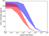 |
Fig. 11 Contrast of the CCF of the |

4 Conclusions and future prospects
High-resolution, ground-based transmission spectra are obtained using double-normalized data reduction techniques. These techniques remove broadband features such as those due to aerosols. Here, we have demonstrated that the contrast difference of the CCF of different absorption bands of water (Δ C), accessible with this kind of measurements, can still be used as a probe of the presence of aerosols. A key factor for the success of this technique is having a broad wavelength coverage, which is provided by current and forthcoming instrumentation (see Sect. 1).
We limited our analysis to the contrast of the CCF, and thus did not consider the full information encoded in the CCF. For example, the broadening of the CCF is a function of temperature, rotation, and atmospheric dynamics. We thus plan to extend our technique to consider the full CCF as a probe of the conditions in the atmosphere. Furthermore, the technique can be extended to other molecular species. Methane is a good candidate as indicator of aerosol-rich atmospheres, as it possess a wealth of absorption bands (that in general do not coincide with the strong water and oxygen telluric absorption bands) that span a broad wavelength range evenly. It can be expected in planets colder than the one simulated here, thus extending the range of cases where our technique can be applied. CO also possesses two absorption bands in the J and K bands, at 1.56 and 2.34 μm, potentially observable in transmission (e.g. Brogi et al. 2016) whose intensity can in principle be compared. They have the advantage that CO is not a strong telluric absorber and of being in the transparency window of Earth; however, with two bands, less information can be extracted by using our technique. On the hot end of the hot Jupiter spectrum (T > 2 000 K), titanium monoxide (TiO) is a good candidate for the same reasons.
Hoeijmakers et al. (2015) and Brogi et al. (2017) demonstrate that, at high-resolution, inaccuracies in molecular line lists propagate to models, introducing uncertainties both in line position and strength (see also a discussion in Pino et al. 2018). While this aspect needs to be thoroughly tested, progress is being made. The ExoMol line list (Tennyson et al. 2016) that contains billions of lines is computationally challenging to use but may possess the required accuracy for this kind of studies (Yurchenko et al. 2008, 2011).
The presence of multiple molecular species with overlapping bands and blended lines might also change the continuum level, and possibly the value of ΔC. However, in the wavelength range considered (λ < 2 μm), only water and titanium monoxide were detected. While other constituents are most likely present, they are undetected, indicating that their signals must be less than the precision of current instrumentation. For this reason, their effect on the continuum should be negligible compared to that of aerosols. Furthermore, TiO is only expected in the hottest atmospheres (Teq ≳ 2000 K). Our technique can thus be safely applied to hot Jupiters with temperatures between about 1000 and 2000 K, but for hotter planets care must be taken in the interpretation of ΔC, and TiO included in the analysis. However, fewer aerosols are expected on this kind of planets (e.g. Heng 2016; Stevenson 2016). In addition, the TiO line list is unreliable at the shortest wavelengths considered in this paper (Hoeijmakers et al. 2015), thus we do not simulate this case.
An extension of the technique to wavelengths λ > 2 μm and to include chromatic scattering by aerosols is warranted, as it may enable the characterization of the composition and size distribution of aerosol particles. Such an extension requires modelling Mie scattering from aerosols and modelling molecular spectral features from multiple species at high resolution.
Acknowledgements
We thank the entire exoplanet atmospheres group of the Geneva Observatory and the Exoplanet and Stellar Populations Group of the University of Padova for insightful discussions. We also thank the anonymous referee, whose constructive critiques sensibly improved the quality of this paper. This work has been carried out in the frame of the National Centre for Competence in Research “PlanetS” supported by the Swiss National Science Foundation (SNSF). L.P., R.A, D.E., C.L., and F.P. acknowledge the financial support of the SNSF. This project has received funding from the European Research Council (ERC) under the European Unions Horizon 2020 research and innovation programme (grant agreement No. 724427).
Appendix A Estimateof photon and telluric noise in CCF observations
A complete assessment of noise sources in real observations of the water CCF is out of the scope of this paper. We do not simulate systematic instrumental effects, since they are different for different instruments, and only partially understood. We stress that having a single instrument able to cover multiple bands such as CARMENES, or a combination of instruments sharing the optics such as HARPS-N + GIANO or HARPS + NIRPS, is generally preferable to combining non-simultaneous observations from different instruments. Instead, we provide estimates of the impact of photon noise and imperfect telluric removal, which are shared by all observations provided by ground-based instrumentation.
A.1 Telluric contamination
In the next future, the kind of observations that we simulated will be carried out only from the ground. We thus estimated the impact of imperfect telluric correction on the simulated observations.
We adopted a telluric transmittance spectrum T1(λ) based on observations of the Sun (Hinkle et al. 2003). We scaled the telluric spectrum, given at air mass 1, at a generic air mass following Vidal-Madjar et al. (2010):
 (A.1)
(A.1)
where a is the target air mass. A transmission spectrum is built by taking the ratio of in- and out-of-transit spectra. We assumed that these are observed at typical air masses 1 and 1.2, respectively. The exact value chosen is not critical. We injected residuals of imperfect telluric correction in our transmission spectra according to
![Mathematical equation: \begin{equation*} \begin{split} \delta_{\mathrm{tell}}(\lambda) \,{=}\,& 1- \left\{1-\mathcal{C}\left[1-\dfrac{T_1}{T_{1.2}}\cdot \lambda\left(1+\dfrac{\mathrm{BERV}}{c}\right)\left(1+\dfrac{v_{\mathrm{syst}}}{c}\right)\right]\right\} \\ & \times(1-\delta(\lambda))\ , \end{split} \end{equation*}](/articles/aa/full_html/2018/11/aa32986-18/aa32986-18-eq30.png) (A.2)
(A.2)
where δ(λ) is the telluric-free model and the telluric spectrum is injected to account for the non-zero systemic velocity of the target star vsyst and the BERV (Barycentric Earth Radial Velocity). For a typical case, we fix vsyst = −2.27 km s-1 as for HD189733b (Boisse et al. 2009) and take a BERV of about 30 km s-1. The constant  ranges between 0 and 1, and represents the quality of the telluric correction. For
  the correction is ideal, that is there are no telluric residuals, for
  there is no correction. We tuned
  in order to have the telluric residual in the simulated HARPS CCF within the noise level on the CCF obtained by Allart et al. (2017) on HD189733b. This is obtained by setting
  , and constitutes a worst-case scenario for the quality of telluric correction with their technique.
It is safe to assume that with ESPRESSO a better quality telluric correction level will be achieved. On the other hand, GIANO data will always be obtained simultaneously to HARPS-N. With the exception of OH emission features, the strongest telluric bands in the NIR are due to the same species that produce them in the optical. Thus, the model transmission spectrum obtained in the optical can be extended to the GIANO wavelength range, and refined with the additional information, to correct for most of the telluric features. In the NIR range, other techniques that exploit the change in the radial velocity of the planet are available (e.g. Brogi et al. 2018). Here, we do not simulate them.
In the  ,
,  and
and  water bands telluric lines saturate, leaving no flux for ground-based observations (see Fig. 1). However, Fig. A.1 shows that the CCF signal is recovered in the
  ,
,  , J and H bands even in the presence of telluric residuals. We note that the
  band is located within a stronger telluric water band, which results in stronger residuals; however, as already mentioned, our estimate of the telluric correction in this region is likely pessimistic since based on HARPS data, of lower quality with respect to what ESPRESSO will provide. The Y band shows some strong telluric residuals that hinder the detection of the exoplanet water feature. However, the same band is accessible at higher resolving power (e.g. CARMENES), and weighted CCF methods (adapted from Baranne et al. 1996; Pepe et al. 2002) may enhance the signal.
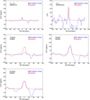 |
Fig. A.1 Effect of telluric contamination on observations of an aerosol-free HD189733b with HARPS-N (upper left panel), ESPRESSO (upper right panel), and GIANO (lower left panel). Red solid line: contamination-free transmission spectrum. Blue solid line: transmission spectrum in the presence of telluric residualso consistent with Allart et al. (2017). If the systemic velocity and the Barycentric Earth Radial Velocity combine such that the exoplanetary signal is shifted away from the telluric residual (here: 30 km s-1), the signal is recovered in the |


It may be surprising that a signal was recovered in the J and H bands, considering the non-negligible absorption by molecular oxygen, carbon dioxide and methane there. This is due to the different structure of the spectrum of these species compared to water. Water has a dense forest of lines, while oxygen, carbon dioxide, and methane have a more symmetrical structure which results in well-separated lines (see Fig. A.2). At the resolution of GIANO, it is thus possible to use the information in-between the lines of these molecules to detect water, even in the absence of any weighting or masking of the telluric lines.
 |
Fig. A.2 Water and molecular oxygen absorption have different properties because of the different structure of the molecules. Upper panel: transmittance of Earth in the J band. The deep telluric lines are from molecular oxygen. They are well separated, and the transmittance approaches 1 between them. Lower panel: an aerosol-free model of HD189733b in the same region. Water generates a dense forest of lines, such that the exoplanetary signal can be recovered from the ground from in-between the deep oxygen telluric lines. |
Value of the dispersion on a single-resolution element in the wings of the CCF of all considered bands for observations of a single transit.
A.2 Photon noise
To estimate the impact of photon noise on the retrieval of the contrast of the CCFs, we simulated observations of HD189733 with the ETCs of ESPRESSO8 and of GIANO9. We assumed
a K2V model for the host star, with magnitudes V = 7.648 and K = 5.541;
seeing 1 arcsec, air mass 1.2, exposure time 300 s;
single HR 2 × 1 slow readout mode for ESPRESSO.
The ETCs provide the signal-to-noise ratio (S/N) on a stellar spectrum in each resolution element,  . We then multiplied this value for the square root of the telluric absorption template from (Hinkle et al. 2003), interpolating on a common grid. By doing so, we accounted for the increased photon noise within the core of the telluric lines. The ETC of GIANO partially accounts for telluric absorption, thus our estimate of the SNR is pessimistic. Finally, the
  on each point of the simulated observations is obtained by
 (A.3)
(A.3)
where Δλobs is the wavelength bin of the simulated observations (see Table 1), Δ λres. elem. is the size of the resolution element in wavelength (computed by the ESPRESSO ETC; 2.7 km s-1 for GIANO), and Ntransit is the number of transits observed. We assumed that the transit duration is 6480 s and neglected overheads. We also assumed that the baseline is observed at a much larger  than the transit. For HARPS, the
  is lowered by
  taking into account the different efficiency and size of the telescope.
These calculations take into account the spectral features of the host star and the decrease of flux in the cores of the individual telluric lines. Not surprisingly, the signal disappears within the  ,
,  and
and  bands. However, in the Y, J, and H bands the signal is confidently recovered (see Fig. A.4).
 |
Fig. A.3 Simulations of observations of an aerosol-free HD189733b with HARPS-N (upper left panel), ESPRESSO (upper right panel) and GIANO (lower left panel). The number of observed transits ranges from 1 (light green) to 9 (purple). A red solid line indincates a noise-free transmission spectrum. While the signal is buried in the photon noise, the combination of 800 water lines results in a detection in the |


 |
Fig. A.4 CCFs obtained measured from the models shown in Fig. A.3. The dispersion values presented in Table A.1 are obtained in the wings of these CCFs. We do not show the |


Table A.1 summarizes the results of our simulations. For each simulated cross-correlation function, we computed the dispersion in its wings, which gives the error on the single resolution element in the velocity space. The results of our simulations are compatible with the precision obtained by Allart et al. (2017) on observations of HD189733b.
Overall, provided that the planet is observed at sufficiently high systemic velocity and BERV, our analysis can be carried out with currentground-based instrumentation. With forthcoming instrumentation mounted at larger telescopes and with a broad spectral coverage, in particular at the ELTs, there is good hope that the photon and systematic noise will abated at the level desired for this kind of analysis.
References
- Allart, R., Lovis, C., Pino, L., et al. 2017, A&A, 606, A144 [NASA ADS] [CrossRef] [EDP Sciences] [Google Scholar]
- Astudillo-Defru, N., & Rojo, P. 2013, A&A, 557, A56 [NASA ADS] [CrossRef] [EDP Sciences] [Google Scholar]
- Baranne, A., Mayor, M., & Poncet, J. L. 1979, Vistas Astron., 23, 279 [NASA ADS] [CrossRef] [Google Scholar]
- Baranne, A., Queloz, D., Mayor, M., et al. 1996, A&AS, 119, 373 [NASA ADS] [CrossRef] [EDP Sciences] [Google Scholar]
- Barstow, J. K., Aigrain, S., Irwin, P. G. J., & Sing, D. K. 2017, ApJ, 834, 50 [Google Scholar]
- Bean, J. L., Miller-Ricci Kempton, E., & Homeier, D. 2010, Nature, 468, 669 [NASA ADS] [CrossRef] [PubMed] [Google Scholar]
- Benneke, B., & Seager, S. 2012, ApJ, 753, 100 [NASA ADS] [CrossRef] [Google Scholar]
- Berta, Z. K., Charbonneau, D., Désert, J.-M., et al. 2012, ApJ, 747, 35 [NASA ADS] [CrossRef] [Google Scholar]
- Birkby, J. L., de Kok, R. J., Brogi, M., et al. 2013, MNRAS, 436, L35 [NASA ADS] [CrossRef] [Google Scholar]
- Boisse, I., Moutou, C., Vidal-Madjar, A., et al. 2009, in Transiting Planets, [Google Scholar]
- Brandl, B. R., Feldt, M., Glasse, A., et al. 2014, Ground-based and Airborne Instrumentation for Astronomy V, Proc. SPIE, 9147, 914721 [Google Scholar]
- Brogi, M., de Kok, R. J., Albrecht, S., et al. 2016, ApJ, 817, 106 [NASA ADS] [CrossRef] [Google Scholar]
- Brogi, M., Line, M., Bean, J., Désert, J.-M., & Schwarz, H. 2017, ApJ, 839, L2 [NASA ADS] [CrossRef] [Google Scholar]
- Brogi, M., Giacobbe, P., Guilluy, G., et al. 2018, A&A, 615, A16 [NASA ADS] [CrossRef] [EDP Sciences] [Google Scholar]
- Charbonneau, D., Brown, T. M., Noyes, R. W., & Gilliland, R. L. 2002, ApJ, 568, 377 [NASA ADS] [CrossRef] [Google Scholar]
- Claudi, R., Benatti, S., Carleo, I., et al. 2017, Eur. Phys. J. Plus, 132, 364 [CrossRef] [Google Scholar]
- Conod, U., Blind, N., Wildi, F., & Pepe, F. 2016, Adaptive Optics Systems V, Proc. SPIE, 9909, 990941 [CrossRef] [Google Scholar]
- Cosentino, R., Lovis, C., Pepe, F., et al. 2012, Ground-based and Airborne Instrumentation for Astronomy IV, Proc. SPIE, 8446, 84461V [CrossRef] [Google Scholar]
- Crepp, J. R., Bechter, A., Bechter, E., et al. 2014, American Astronomical Society Meeting Abstracts, 223, 348.20 [Google Scholar]
- Crossfield, I. J. M. 2014, A&A, 566, A130 [NASA ADS] [CrossRef] [EDP Sciences] [Google Scholar]
- Crossfield, I. J. M. 2015, PASP, 127, 941 [NASA ADS] [CrossRef] [Google Scholar]
- de Kok, R. J., Brogi, M., Snellen, I. A. G., et al. 2013, A&A, 554, A82 [NASA ADS] [CrossRef] [EDP Sciences] [Google Scholar]
- de Kok, R. J., Birkby, J., Brogi, M., et al. 2014, A&A, 561, A150 [NASA ADS] [CrossRef] [EDP Sciences] [Google Scholar]
- de Mooij, E. J. W., Brogi, M., de Kok, R. J., et al. 2013, ApJ, 771, 109 [NASA ADS] [CrossRef] [Google Scholar]
- Deming, D., & Sheppard, K. 2017, ApJ, 841, L3 [NASA ADS] [CrossRef] [Google Scholar]
- Désert, J.-M., Lecavelier des Etangs, A., Hébrard, G., et al. 2009, ApJ, 699, 478 [NASA ADS] [CrossRef] [Google Scholar]
- Di Gloria, E., Snellen, I. A. G., & Albrecht, S. 2015, A&A, 580, A84 [NASA ADS] [CrossRef] [EDP Sciences] [Google Scholar]
- Ehrenreich, D., Tinetti, G., Lecavelier Des, A., Vidal-Madjar, A., & Selsis, F. 2006, A&A, 448, 379 [NASA ADS] [CrossRef] [EDP Sciences] [Google Scholar]
- Ehrenreich, D., Vidal-Madjar, A., Widemann, T., et al. 2012, A&A, 537, L2 [NASA ADS] [CrossRef] [EDP Sciences] [Google Scholar]
- Ehrenreich, D., Bonfils, X., Lovis, C., et al. 2014, A&A, 570, A89 [NASA ADS] [CrossRef] [EDP Sciences] [Google Scholar]
- Esteves, L. J., de Mooij, E. J. W., Jayawardhana, R., Watson, C., & de Kok R. 2017, AJ, 153, 268 [NASA ADS] [CrossRef] [Google Scholar]
- Follert, R., Dorn, R. J., Oliva, E., et al. 2014, Ground-based and Airborne Instrumentation for Astronomy V, Proc. SPIE, 9147, 914719 [Google Scholar]
- France, K., Fleming, B., West, G., et al. 2017, in Society of Photo-Optical Instrumentation Engineers (SPIE) Conference Series, 10397, 1039713 [Google Scholar]
- Gibson, N. P., Nikolov, N., Sing, D. K., et al. 2017, MNRAS, 467, 4591 [NASA ADS] [CrossRef] [Google Scholar]
- Grimm, S. L., & Heng, K. 2015, ApJ, 808, 182 [NASA ADS] [CrossRef] [Google Scholar]
- Heng, K. 2016, ApJ, 826, L16 [NASA ADS] [CrossRef] [Google Scholar]
- Heng, K., & Kitzmann, D. 2017, MNRAS, 470, 2972 [NASA ADS] [CrossRef] [Google Scholar]
- Heng, K., Wyttenbach, A., Lavie, B., et al. 2015, ApJ, 803, L9 [Google Scholar]
- Hinkle, K. H., Wallace, L., & Livingston, W. 2003, BAAS, 35, 1260 [NASA ADS] [Google Scholar]
- Hoeijmakers, H. J., de Kok, R. J., Snellen, I. A. G., et al. 2015, A&A, 575, A20 [NASA ADS] [CrossRef] [EDP Sciences] [Google Scholar]
- Jurgenson, C., Fischer, D., McCracken, T., et al. 2016, Ground-based and Airborne Instrumentation for Astronomy VI, Proc. SPIE, 9908, 99086T [Google Scholar]
- Kotani, T., Tamura, M., Suto, H., et al. 2014, Ground-based and Airborne Instrumentation for Astronomy V, Proc. SPIE, 9147, 914714 [Google Scholar]
- Kreidberg, L., Bean, J. L., Désert, J.-M., et al. 2014a, Nature, 505, 69 [NASA ADS] [CrossRef] [Google Scholar]
- Kreidberg, L., Bean, J. L., Désert, J.-M., et al. 2014b, ApJ, 793, L27 [NASA ADS] [CrossRef] [Google Scholar]
- Lecavelier Des, A., Pont, F., Vidal-Madjar, A., & Sing, D. 2008, A&A, 481, L83 [NASA ADS] [CrossRef] [Google Scholar]
- Lendl, M., Delrez, L., Gillon, M., et al. 2016, A&A, 587, A67 [NASA ADS] [CrossRef] [EDP Sciences] [Google Scholar]
- Mahadevan, S., Ramsey, L., Bender, C., et al. 2012, Ground-based and Airborne Instrumentation for Astronomy IV, Proc. SPIE, 8446, 84461S [CrossRef] [Google Scholar]
- Marconi, A., Di Marcantonio, P., D’Odorico, V., et al. 2016, Ground-based and Airborne Instrumentation for Astronomy VI, Proc. SPIE, 9908, 990823 [Google Scholar]
- Mayor, M., Pepe, F., Queloz, D., et al. 2003, Messenger, 114, 20 [Google Scholar]
- McCarthy, D. W., Burge, J. H., Angel, J. R. P., et al. 1998, Infrared Astronomical Instrumentation, ed. A. M. Fowler, Proc. SPIE, 3354, 750 [NASA ADS] [CrossRef] [Google Scholar]
- Miguel, Y., & Kaltenegger, L. 2014, ApJ, 780, 166 [NASA ADS] [CrossRef] [Google Scholar]
- Mollière, P., van Boekel, R., Bouwman, J., et al. 2017, A&A, 600, A10 [NASA ADS] [CrossRef] [EDP Sciences] [Google Scholar]
- Nascimbeni, V., Piotto, G., Pagano, I., et al. 2013, A&A, 559, A32 [NASA ADS] [CrossRef] [EDP Sciences] [Google Scholar]
- Oliva, E., Origlia, L., Baffa, C., et al. 2006, Society of Photo-Optical Instrumentation Engineers (SPIE) Conference Series, Proc. SPIE, 6269, 626919 [CrossRef] [Google Scholar]
- Pepe, F., Mayor, M., Galland, F., et al. 2002, A&A, 388, 632 [NASA ADS] [CrossRef] [EDP Sciences] [Google Scholar]
- Pepe, F. A., Cristiani, S., Rebolo Lopez, R., et al. 2010, Ground-based and Airborne Instrumentation for Astronomy III, Proc. SPIE, 7735, 77350F [CrossRef] [Google Scholar]
- Pinhas, A., & Madhusudhan, N. 2017, MNRAS, 471, 4355 [NASA ADS] [CrossRef] [Google Scholar]
- Pino, L., Ehrenreich, D., Wyttenbach, A., et al. 2018, A&A, 612, A53 [NASA ADS] [CrossRef] [EDP Sciences] [Google Scholar]
- Pont, F., Sing, D. K., Gibson, N. P., et al. 2013, MNRAS, 432, 2917 [NASA ADS] [CrossRef] [Google Scholar]
- Press, W. H., Flannery, B. P., Teukolsky, S. A., & Vetterling, W. T. 1989, Numerical Recipes in C. The Art of Scientific Computing (Cambridge, UK: Cambridge University Press) [Google Scholar]
- Quirrenbach, A., Amado, P. J., Caballero, J. A., et al. 2014, Ground-based and Airborne Instrumentation for Astronomy V, Proc. SPIE, 9147, 91471F [Google Scholar]
- Schwab, C., Rakich, A., Gong, Q., et al. 2016, Ground-based and Airborne Instrumentation for Astronomy VI, Proc. SPIE, 9908, 99087H [Google Scholar]
- Sharp, C. M., & Burrows, A. 2007, ApJS, 168, 140 [NASA ADS] [CrossRef] [Google Scholar]
- Sing, D. K., Wakeford, H. R., Showman, A. P., et al. 2015, MNRAS, 446, 2428 [NASA ADS] [CrossRef] [Google Scholar]
- Sing, D. K., Fortney, J. J., Nikolov, N., et al. 2016, Nature, 529, 59 [NASA ADS] [CrossRef] [Google Scholar]
- Snellen, I. A. G. 2004, MNRAS, 353, L1 [NASA ADS] [CrossRef] [Google Scholar]
- Snellen, I. A. G., Albrecht, S., de Mooij, E. J. W., & Le Poole R. S. 2008, A&A, 487, 357 [NASA ADS] [CrossRef] [EDP Sciences] [Google Scholar]
- Snellen, I. A. G., de Kok, R. J., de Mooij, E. J. W., & Albrecht, S. 2010, Nature, 465, 1049 [NASA ADS] [CrossRef] [PubMed] [Google Scholar]
- Snellen, I. A. G., de Kok, R. J., le Poole, R., Brogi, M., & Birkby, J. 2013, ApJ, 764, 182 [NASA ADS] [CrossRef] [Google Scholar]
- Stevenson, K. B. 2016, ApJ, 817, L16 [NASA ADS] [CrossRef] [Google Scholar]
- Strassmeier, K. G., Ilyin, I., Järvinen, A., et al. 2015, Astron. Nachr., 336, 324 [NASA ADS] [CrossRef] [Google Scholar]
- Szentgyorgyi, A., Frebel, A., Furesz, G., et al. 2012, Ground-based and Airborne Instrumentation for Astronomy IV, Proc. SPIE, 8446, 84461H [CrossRef] [Google Scholar]
- Szentgyorgyi, A., Barnes, S., Bean, J., et al. 2014, Ground-based and Airborne Instrumentation for Astronomy V, Proc. SPIE, 9147, 914726 [Google Scholar]
- Tennyson, J., Yurchenko, S. N., Al-Refaie, A. F., et al. 2016, J. Mol. Spectr., 327, 73 [NASA ADS] [CrossRef] [Google Scholar]
- Thibault, S., Rabou, P., Donati, J.-F., et al. 2012, Ground-based and Airborne Instrumentation for Astronomy IV, Proc. SPIE, 8446, 844630 [CrossRef] [Google Scholar]
- TMT Project. 2013, TMT Science-based Requirements Document, TMT document number TMT.PSC.DRD.05.001.CCR19, Tech. Rep. [Google Scholar]
- Todorov, K. O., Line, M. R., Pineda, J. E., et al. 2016, ApJ, 823, 14 [NASA ADS] [CrossRef] [Google Scholar]
- Vidal-Madjar, A., Arnold, L., Ehrenreich, D., et al. 2010, A&A, 523, A57 [NASA ADS] [CrossRef] [EDP Sciences] [Google Scholar]
- Wakeford, H. R., & Sing, D. K. 2015, A&A, 573, A122 [NASA ADS] [CrossRef] [EDP Sciences] [Google Scholar]
- Wakeford, H. R., Stevenson, K. B., Lewis, N. K., et al. 2017, ApJ, 835, L12 [NASA ADS] [CrossRef] [Google Scholar]
- Wakeford, H. R., Sing, D. K., Deming, D., et al. 2018, AJ, 155, 29 [Google Scholar]
- Wright, J. T., & Robertson, P. 2017, Res. Notes Am. Astron. Soc., 1, 51 [CrossRef] [Google Scholar]
- Wyttenbach, A., Ehrenreich, D., Lovis, C., Udry, S., & Pepe, F. 2015, A&A, 577, A62 [NASA ADS] [CrossRef] [EDP Sciences] [Google Scholar]
- Wyttenbach, A., Lovis, C., Ehrenreich, D., et al. 2017, A&A, 602, A36 [NASA ADS] [CrossRef] [EDP Sciences] [Google Scholar]
- Yuk, I.-S., Jaffe, D. T., Barnes, S., et al. 2010, Ground-based and Airborne Instrumentation for Astronomy III, Proc. SPIE, 7735, 77351M [CrossRef] [Google Scholar]
- Yurchenko, S. N., Voronin, B. A., Tolchenov, R. N., et al. 2008, J. Chem. Phys., 128, 044312 [NASA ADS] [CrossRef] [Google Scholar]
- Yurchenko, S. N., Barber, R. J., Tennyson, J., Thiel, W., & Jensen, P. 2011, J. Mol. Spectr., 268, 123 [NASA ADS] [CrossRef] [Google Scholar]
- Zerbi, F. M., Bouchy, F., Fynbo, J., et al. 2014, Ground-based and Airborne Instrumentation for Astronomy V, Proc. SPIE, 9147, 914723 [Google Scholar]
The optical and NIR spectral range will be covered by JWST NIRSpec, which will provide a resolving power of R ~ 103. This is by two orders of magnitude lower than the resolving power that ground-based facilities can provide.
A discussion of the theoretical water spectrum can be found at http://www1.lsbu.ac.uk/water/water_vibrational_spectrum.html and references therein.
More precisely, we perform cross-correlation as defined in the field of signal processing, which is a measure of similarity between two signals (the binary mask and the data, e.g. Press et al. 1989). The terminology in signal processing differs from the terminology in statistics, where the cross-correlation is normalized by the variance of the data. It should be noted that works by other groups, e.g. Snellen et al. (2010), adopt the CCF as defined in statistics, that is normalized by the variance of the two signals. The two definitions of CCF differ just by a normalization factor, and the adoption of one or the other definition should not impact our conclusions.
To rescale the lines intensity we used the partition function provided by HITRAN: http://hitran.iao.ru/partfun. We note also that the spectral line intensity parameter of HITEMP represents the area below the spectral line. If a strong line is also broadened it may be less optimal for the CCF analysis than a weaker but narrow line. We consider this effect negligible when selecting 800 lines.
This was verified by repeating the whole analysis with a mask at a temperature of 2100 K, and by keeping the 400 and 1600 most intense lines (in place of 800).
Either of the two can be arbitrarily fixed, and the other becomes a free parameter.
All Tables
Typical CCF contrast difference (ΔC) between pairs of water bands and pressure range where this maximum difference is reached.
Typical CCF contrast difference (ΔC) between pairs of water bands and pressure range where this maximum difference is reached when considering regions where telluric correction is possible.
Value of the dispersion on a single-resolution element in the wings of the CCF of all considered bands for observations of a single transit.
All Figures
|
Fig. 1 Bands used to compute the CCF of water, on top of the telluric transmittance (upper panel), and an exoplanet transmission spectrum model (lower panel). Grey bands correspond to water vibrational band. Orange bands correspond to the windows of transparency of Earth atmosphere. The bands partially overlap, as indicated by toothed areas. Upper panel: the solid black line represents the transmittance of Earth atmosphere (Hinkle et al. 2003), ranging from 1 (all incident light transmitted) to 0 (all incident light absorbed). Besides water bands, corresponding to the bands in the bottom panel, molecular oxygen, carbon dioxide, and methane show the most prominent features. Lower panel: the solid black line represents a theoretical cloud-free isothermal model of HD189733b. Within each water vibrational band, the region of the spectrum in grey represents the spectrum seen through a selected instrument, thus convolved at the appropriate resolving power (see Table 1). |
| In the text | |
|
Fig. 2 Effect of finite resolving power on water lines. The red curve corresponds to a line-by-line model (with a resolution of R ~ 106). From the light green curve to the purple curve, we show the same spectrum convolved with Gaussian LSF corresponding to the following resolving powers: at R = 50 000 (GIANO), at R = 75 000 (similar to CARMENES), at R = 115 000 (HARPS/-N), and at R = 134 000 (ESPRESSO). At the lowest resolving power, the individual molecular lines are not entirely resolved. |
| In the text | |
|
Fig. 3 CCFs for the |
| In the text | |
|
Fig. 4 Contrast of the CCF as a function of altitude of aerosols (expressed as pressure of the cloud top). Lighter colours indicate colder models, darker colours indicate hotter models (between 1200 and 2300 K), as indicated by the colour-matched labels. Left panel: |
| In the text | |
|
Fig. 5 Temperature dependence of the high-resolution transmission spectrum of a hot Jupiter. The temperature varies between 1200 and 2300 K in steps of ~200 K (from light to dark). Left panel: zoom on one line of the sodium doublet. The contrast of the sodium feature in the hottest atmosphere (purple) is approximately twice its contrast in the coldest atmosphere (light green). This behaviour is explained through the linear dependence of atmospheric signal on temperature through the scale height. Right panel: zoom on a region of the
|
| In the text | |
|
Fig. 6 Results in the ideal case. Upper panel: high-resolution models of a hot Jupiter with T = 1700 K and differentvalues of pc, ranging between 10−7 and 1 bar. Each colour corresponds to a different value of pc, and the lightest colours correspond to condensates deeper in the atmosphere. Lower panel: CCF contrast as a function of wavelength. The colours are in correspondence with the models shown in the upper panel. For each value of pc, the temperature range 1200–2300 K is explored. We indicate with a vertical error bar the induced variation in the contrast of the CCF. On the left, the 1-pixel, 1σ precision of HARPS (blue) and ESPRESSO (green) for a single transit are shown. These error bars only account for photon noise, but telluric residuals may introduce additional noise (see Appendix A). The NIR bands must be accessed from space or from the stratosphere. Such instruments do not yet exist, and we do not estimate an error bar. |
| In the text | |
|
Fig. 7 Difference in contrast between the CCF of the |
| In the text | |
|
Fig. 8 Sensitivity of different combinations of water bands to the presence of aerosols. Each panel shows the difference between the band highlighted in the bottom row and the band highlighted in the left column. The x- and y-axes are the same as for Fig. 7, running between 1 and 10−7 bar and between 0 and 300 ppm, respectively. Orange and green horizontal dashed lines are put in correspondence to the 100 and 200 ppm levels. |
| In the text | |
|
Fig. 9 CCF contrast as a function of wavelength in the case where telluric contamination is considered, in the presence of a grey opacity source simulating large condensates at various pressure levels. Upper panel: high-resolution models of a hot Jupiter with T = 1700 K. Each colour corresponds to a different value of pc, ranging between 10−7 and 1 bar, and the lightest colours correspond to condensates deeper in the atmosphere. Lower panel: CCF contrast as a function of wavelength. The colours are in correspondence with the models shown in the upper panel. For each value of pc, the temperature range 1200–2300 K is explored. We indicate with a vertical error bar the induced variation in the contrast of the CCF. On the left, the 1σ precision of HARPS (blue), ESPRESSO (green), GIANO (orange, red, and black) for the Y, J, and H bands for a single transit are shown. These error bars only account for photon noise, but telluric residuals may introduce additional noise (see Appendix A). |
| In the text | |
|
Fig. 10 Sensitivity to the presence of aerosols of different combinations of bands that are accessible from the ground even in the presence of tellurics. Each panel shows the difference between the band highlighted in the bottom row and the band highlighted in the left column. The x- and y-axes are the same as for Fig. 7, running between 1 and 10−7 bar and between 0 and 300 ppm, respectively. Orange and green horizontal dashed lines are put in correspondence to the 100 and 200 ppm levels. We note that these values are arbitrary. Scatterers up to the 0.1 mbar level produce values of ΔC up to 100 ppm. |
| In the text | |
|
Fig. 11 Contrast of the CCF of the |
| In the text | |
|
Fig. A.1 Effect of telluric contamination on observations of an aerosol-free HD189733b with HARPS-N (upper left panel), ESPRESSO (upper right panel), and GIANO (lower left panel). Red solid line: contamination-free transmission spectrum. Blue solid line: transmission spectrum in the presence of telluric residualso consistent with Allart et al. (2017). If the systemic velocity and the Barycentric Earth Radial Velocity combine such that the exoplanetary signal is shifted away from the telluric residual (here: 30 km s-1), the signal is recovered in the |
| In the text | |
|
Fig. A.2 Water and molecular oxygen absorption have different properties because of the different structure of the molecules. Upper panel: transmittance of Earth in the J band. The deep telluric lines are from molecular oxygen. They are well separated, and the transmittance approaches 1 between them. Lower panel: an aerosol-free model of HD189733b in the same region. Water generates a dense forest of lines, such that the exoplanetary signal can be recovered from the ground from in-between the deep oxygen telluric lines. |
| In the text | |
|
Fig. A.3 Simulations of observations of an aerosol-free HD189733b with HARPS-N (upper left panel), ESPRESSO (upper right panel) and GIANO (lower left panel). The number of observed transits ranges from 1 (light green) to 9 (purple). A red solid line indincates a noise-free transmission spectrum. While the signal is buried in the photon noise, the combination of 800 water lines results in a detection in the |
| In the text | |
|
Fig. A.4 CCFs obtained measured from the models shown in Fig. A.3. The dispersion values presented in Table A.1 are obtained in the wings of these CCFs. We do not show the |
| In the text | |
Current usage metrics show cumulative count of Article Views (full-text article views including HTML views, PDF and ePub downloads, according to the available data) and Abstracts Views on Vision4Press platform.
Data correspond to usage on the plateform after 2015. The current usage metrics is available 48-96 hours after online publication and is updated daily on week days.
Initial download of the metrics may take a while.