| Issue |
A&A
Volume 619, November 2018
|
|
|---|---|---|
| Article Number | A160 | |
| Number of page(s) | 18 | |
| Section | Planets and planetary systems | |
| DOI | https://doi.org/10.1051/0004-6361/201732332 | |
| Published online | 20 November 2018 | |
High-contrast study of the candidate planets and protoplanetary disk around HD 100546★
1
INAF – Osservatorio Astronomico di Padova, Vicolo dell’Osservatorio 5,
35122,
Padova, Italy
e-mail: This email address is being protected from spambots. You need JavaScript enabled to view it.
2
Dipartimento di Fisica e Astronomia – Universita’ di Padova, Vicolo dell’Osservatorio 3,
35122,
Padova, Italy
3
Institute for Particle Physics and Astrophysics, ETH Zurich,
Wolfgang-Pauli-Strasse 27, CH-8093 Zurich, Switzerland
4
Departamento Física Teórica, Universidad Autonóma de Madrid,
Módulo 15, Facultad de Ciencias, Campus de Cantoblanco,
28049,
Madrid, Spain
5
Núcleo de Astronomía, Facultad de Ingeniería, Universidad Diego Portales,
Av. Ejercito 441, Santiago, Chile
6
Aix-Marseille Université, CNRS, LAM (Laboratoire d’Astrophysique de Marseille) UMR 7326,
13388, Marseille, France
7
University of Atacama,
Copayapu 485,
Copiapo, Chile
8
CRAL, UMR 5574, CNRS, Université de Lyon,
Ecole Normale Supérieure de Lyon, 46 Allée d’Italie,
69364
Lyon Cedex 07, France
9
Leiden Observatory, Leiden University,
PO Box 9513,
2300 RA Leiden, The Netherlands
10
Université Grenoble Alpes, CNRS, IPAG,
38000 Grenoble, France
11
Max-Planck-Institut für Astronomie,
Königstuhl 17,
69117 Heidelberg, Germany
12
INAF – Osservatorio Astrofisico di Arcetri,
L.go E. Fermi 5,
50125 Firenze, Italy
13
Institute for Astronomy, University of Edinburgh,
Blackford Hill, Edinburgh EH9 3HJ, UK
14
LESIA, Observatoire de Paris-Meudon, CNRS, Université Pierre et Marie Curie, Université Paris Diderot,
5 Place Jules Janssen,
92195 Meudon, France
15
INAF – Osservatorio Astrofisico di Catania,
Via S. Sofia 78,
95123 Catania, Italy
16
INAF – Osservatorio Astronomico di Capodimonte,
Via Moiariello 16,
80131 Napoli, Italy
17
Unidad Mixta Internacional Franco-Chilena de Astronomia, CNRS/INSU UMI 3386 and Departamento de Astronomia, Universidad de Chile,
Casilla 36-D,
Santiago, Chile
18
Observatoire de Genéve, University of Geneva,
51 Chemin des Maillettes, 1290,
Versoix, Switzerland
19
INAF – Osservatorio Astronomico di Brera,
via Emilio Bianchi 46,
23807,
Merate (LC), Italy
20
INAF – Istituto di Astrofisica Spaziale e Fisica Cosmica di Milano,
Via E. Bassini 15,
20133 Milano, Italy
21
Department of Astronomy, Stockholm University,
SE-106 91 Stockholm, Sweden
22
European Southern Observatory,
Karl-Schwarzschild-Str. 2,
D85748 Garching, Germany
23
Laboratoire Lagrange (UMR 7293), UNSA, CNRS, Observatoire de la Côte d’Azur, Bd. de l’Observatoire,
06304 Nice Cedex 4, France
24
Department of Astronomy, University of Michigan, 311 West Hall, 1085 S. University Avenue,
Ann Arbor,
MI 48109, USA
Received:
21
November
2017
Accepted:
30
August
2018
Abstract
The nearby Herbig Be star HD 100546 is known to be a laboratory for the study of protoplanets and their relation with the circumstellar disk, which is carved by at least two gaps. We observed the HD 100546 environment with high-contrast imaging exploiting several different observing modes of SPHERE, including data sets with and without coronagraphs, dual band imaging, integral field spectroscopy and polarimetry. The picture emerging from these different data sets is complex. Flux-conservative algorithm images clearly show the disk up to 200 au. More aggressive algorithms reveal several rings and warped arms that are seen overlapping the main disk. Some of these structures are found to lie at considerable height over the disk mid-plane at about 30 au. Our images demonstrate that the brightest wings close to the star in the near side of the disk are a unique structure, corresponding to the outer edge of the intermediate disk at ~ 40 au. Modeling of the scattered light from the disk with a geometrical algorithm reveals that a moderately thin structure (H∕r = 0.18 at 40 au) can well reproduce the light distribution in the flux-conservative images. We suggest that the gap between 44 and 113 au spans between the 1:2 and 3:2 resonance orbits of a massive body located at ~ 70 au, which mightcoincide with the candidate planet HD 100546b detected with previous thermal infrared (IR) observations. In this picture, the two wings can be the near side of a ring formed by disk material brought out of the disk at the 1:2 resonance with the same massive object. While we find no clear evidence confirming detection of the planet candidate HD 100546c in our data, we find a diffuse emission close to the expected position of HD 100546b. This source can be described as an extremely reddened substellar object surrounded by a dust cloud or its circumplanetary disk. Its astrometry is broadly consistent with a circular orbital motion on the disk plane, a result that could be confirmed with new observations. Further observations at various wavelengths are required to fully understand the complex phenomenology of HD 100546.
Key words: stars: individual: HD 100546 / techniques: high angular resolution / techniques: polarimetric / protoplanetary disks / planets and satellites: detection
Based on data collected at the European Southern Observatory, Chile (ESO Programs 095.C-0298, 096.C-0241, 096.C-0248, 097.C-0523, 097.C-0865, and 098.C-0209).
© ESO 2018
1 Introduction
The number of known exoplanets around main sequence stars is rapidly increasing. However, the number of detected (forming) exoplanets around pre-main sequence stars remains low. Possibly the best examples are LkCa 15 (Kraus & Ireland 2012; Sallum et al. 2015), HD 169142 (Biller et al. 2014; Reggiani et al. 2014), HD 100546 (Quanz et al. 2013, 2015; Currie et al. 2014, 2015; Rameau et al. 2017), and PDS 70 (Keppler et al. 2018; Müller et al. 2018). To understand the formation process of planets, we need to study the initial conditions and evolution of circumstellar disks, and how the disk can be shaped by ongoing planet formation.
Recently developed high-contrast and high-angular-resolution imaging instruments such as SPHERE (Spectro-Polarimetric High-contrast Exoplanet REsearch; Beuzit et al. 2008), GPI (Gemini Planet Imager; Macintosh et al. 2014), SCExAO (Subaru Coronagraphic Extreme Adaptive Optics; Jovanovic et al. 2015) and FLAO (First Light AO system; Quirós-Pacheco et al. 2010) provide the excellent capability to directly obtain images of protoplanetary disks around nearby young stars, up to the inner tens of astronomical units, in scattered light and thermal emission. This sometimes makes it possible to observe planets in their birthplace and to investigate their interaction with the disk. Imaging protoplanetary disks around young stars allows us to detect spiral structures and gaps which might be produced by gravitational perturbation of forming planets, as demonstrated by Grady et al. (2001), Thalmann et al. (2010), Garufi et al. (2013), Pinilla et al. (2015) and Dong et al. (2016), for example.
HD 100546 is a nearby (d = 109 ± 4 pc; Gaia Collaboration 2016) well-studied Herbig Be star with spectral type B9Vne (Levenhagen & Leister 2006) which harbours a large disk. Several studies have been conducted in the past years on this disk, from spectroscopic and photometric analyses to direct imaging. The first evidence of the presence of the disk around HD 100546 was obtained by Hu et al. (1989) measuring the infrared (IR) excess in the spectral energy distribution (SED). The mid-IR (MIR) excess in the SED of this source requires a thickening of the disk at ~ 0.1′′, which can be explained by a proto-Jupiter carving a gap (Bouwman et al. 2003). This idea is also supported by far-ultraviolet (FUV) long-slit spectroscopy with HST/STIS, which detected a central cavity up to 0.13′′ (Grady et al. 2005), by UVES observations of [OI] emission region (Acke & van den Ancker 2006) using spectro-astrometry with CO roto-vibrational emission by van der Plas et al. (2009), and by AMBER/VLTI observations in the K-band (Benisty et al. 2010).
The disk was first imaged in scattered light in the J and K bands with the adaptive optics system ADONIS coupled with a pre-focal optics coronagraph (Pantin et al. 2000). The disk was detected up to 2′′ from the star, with a density peak at ~40 au. Many successive works revealed the complexity of its geometry by means of both scattered light images (e.g. Augereau et al. 2001; Ardila et al. 2007; Quanz et al. 2011; Garufi et al. 2016; Follette et al. 2017) and also (sub-)millimeter images (e.g. Walsh et al. 2014; Pineda et al. 2014; Wright et al. 2015). The radial profile of the disk brightness becomes less steep at separations < 2.7′′ in both HST/NICMOS2 H-band (Augereau et al. 2001) and ADONIS Ks (Grady et al. 2001) band. However this change is not visible in the optical. Moreover, the semi-minor axis brightness profile is asymmetric in the H-band (Augereau et al. 2001); this can be related to an optically thick circumstellar disk inside 0.8′′ and an optically thin disk at larger separations.
Thanks to the higher angular resolution reachable with HST/STIS coronagraphic images, the first disk structures were detected: spiral dark filaments appear mostly in the SW at separations greater than 2.3′′ (Grady et al. 2001). Following observations revealed additional spiral structures both at short and long separations, possibly related to forming planets (Ardila et al. 2007; Boccaletti et al. 2013; Currie et al. 2015; Garufi et al. 2016). The first polarimetric differential imaging (PDI) detection of the disk (Quanz et al. 2011) in H and Ks NACO filters resolved the disk between 0.1′′ and 1.4′′, locating the disk inner rim at 0.15′′. They noted an asymmetry along the brightness profile that they interpreted as the presence of two dust populations. Deeper observations by Avenhaus et al. (2014) reached the innermost region (~ 0.03′′) and found aspiral arm in the far side of the disk. The disk is found to be strongly flared in the outer regions (> 80–100 au) and is expected to generate a shadowing effect on the forward-scattering side of the disk. The disk appears faint and red due to the combination of particle sizes and disk geometry as demonstrated by Mulders et al. (2013) and later confirmed by Stolker et al. (2016) comparing models to PDI data.
In addition to these data from the disk, several studies suggest that HD 100456 may host at least two planets (Quanz et al. 2013, 2015; Brittain et al. 2014; Currie et al. 2015) located at ~ 55 au (hereafter CCb) and ~13 au (hereafter CCc) from the central star. This makes the system a powerful laboratory to study planet formation and planet–disk interaction.
Quanz et al. (2015) inferred the temperature and emitting radius of CCb in the L′ and M bands and concluded that what they imaged could be a warm circumplanetary disk rather than the planet itself. An extended emission at near-infrared (NIR) wavelengths, possibly linked with this candidate planet was also detected by Currie et al. (2015) centred at 0.469±0.012′′, PA = 7.04° ± 1.39°. Its infrared colours are extremely red compared to models, indicating that it could still be embedded by accreting material.
The existence of CCc was proposed by Brittain et al. (2013), who ascribed the variability of the CO ro-vibrational lines to a compact source of emission at ~15 au from the central star. Currie et al. (2015) showed that this object is detected in GPI H-band images. However, there is a debate over this result, because detection strongly depends on the reduction method used (see e.g. Garufi et al. 2016; Follette et al. 2017; Currie et al. 2017) and on its nature, since it can be interpreted with alternative equally plausible origins like disk hot spot or an indirect signature of the presence of the planet.
The first observations of HD 100546 with VLT/SPHERE were presented in Garufi et al. (2016), where it was found that the disk around HD 100546 is truncated at about 11 au and the cavity is consistent with being intrinsically circular. More recent works by Follette et al. (2017), Rameau et al. (2017) and Currie et al. (2017), all based on GPI data sets, debate on the presence of both the planets and the impact of the reduction methods on them.
HD 100546 is located in the Sco-Cen complex. In this analysis we consider a stellar mass of M* = 2.4 M⊙ (Brittain et al. 2014), and apparent magnitudes of J = 6.42, H = 5.96, and K = 5.42 (Cutri et al. 2003), as well as L′ = 4.52 and M′ = 4.13 as in Quanz et al. (2015). For the disk, we assume an inclination i = 42° (Ardila et al. 2007; Pineda et al. 2014) and PA = 146° (Pineda et al. 2014).
In this paper, we present the results of a two-year observational campaign on this star, based on observations in direct imaging with VLT/SPHERE, the new high-contrast and high-resolution instrument dedicated to exoplanet and disk imaging, that includes both pupil tracking and polarimetric observations. SPHERE includes a powerful extreme adaptive optics system (Sphere AO for eXoplanet Observation, SAXO; Fusco et al. 2006), providing a currently unmatched Strehl Ratio of up to 92% in the H-band for bright (R < 9) sources, various coronagraphs (see Martinez et al. 2009; Carbillet et al. 2011), an infrared differential imaging camera (IRDIS; Dohlen et al. 2008), an infrared integral field spectrograph (IFS; Claudi et al. 2008) and a visible differential polarimeter and imager (ZIMPOL; Thalmann et al. 2008).
The paper is structured as follows. The observing strategy, sky conditions, and the reduction of these data set are described in Sect. 2. The results for the disk and planets are given in Sects. 3 and 4, respectively. Conclusions are given in Sect. 5.
2 Observations and data reduction
2.1 Observations
We observed HD 100546 at different epochs as part of the SHINE (SpHere INfrared survey for Exoplanets) guaranteed time observations(GTO) program using IRDIS and IFS simultaneously: the IRDIFS mode (with IFS operating between 0.95 and 1.35 μm and IRDIS working in dual imaging mode in the H2H3 filter pair at 1.59 and 1.67 μm ; Vigan et al. 2010) and the IRDIFS_EXT mode (with IFS operating at Y–H wavelengths 0.95–1.65 μm and IRDIS in the K1K2 band filters at 2.11 and 2.25 μm). These observations were all carried-out with the N_ALC_YJH_S apodized Lyot coronagraph (inner working angle, IWA ~ 0.1′′ ; Boccaletti et al. 2008)except for two sequences which were acquired without coronagraph in order to study the central region (at less than 0.1′′ from the star). Inthis case, to avoid heavy saturation of the star, a neutral density filter with average transmission ~1/100 was used. All data were taken in pupil stabilised mode in order to perform angular differential imaging (ADI, see e.g. Marois et al. 2006)for subtracting the stellar residuals.
HD 100546 was also observed in PDI (see e.g. Kuhn et al. 2001; Quanz et al. 2011) as part of the DISK GTO program, using IRDISwith the same coronagraphic mask as for the classical imaging. The source was observed for a total time of 21 min in the J band (1.26 μm) and 38 min in the K band (2.181 μm) during the night of March 31, 2016 and May 25, 2016, respectively. The orientation of the derotator was chosen in order to optimise thepolarimetric efficiency of IRDIS (de Boer et al., in prep.).
Several of the observations were carried out under moderate and good weather conditions (with an average coherence time, τ0, longer than 2.0 ms). Details on the full set of observations are presented in Table 1; τ0 and Strehl ratio were measured by SPARTA, the ESO standard real-time computer platform that controls the AO loop.
In order to access the quality of the observational material, we plotted in Fig. 1 the contrast we achieved in the IFS raw images as a function of the separation for all the non-polarimetric images except March 2016 data set, due to its very unstable sky conditions. The contrasts plotted here were obtained combining the root mean square scatter of a 1λ∕D diameter spot along a 1λ∕D wide annulus, at different separation from the star as described in Mesa et al. (2015). These contrast values were then corrected for the low-number statistics according to Mawet et al. (2014). We noticed that these raw image contrasts are comparable to those obtained with the two GPI data sets presented in Currie et al. (2017).
We found that the highest-quality coronagraphic observations are those from May 2015 to May 2016 while the observationsobtained in January and March 2016 are of poor quality due to the atmospheric conditions or low system performances (calibration of the deformable mirror voltages was not optimal in January 2016). For the non-coronagraphic data sets, the lack of a coronagraph implies much stronger diffraction patterns and the need for using the neutral density filter, common to IFS and IRDIS, to avoid saturation close to the centre; this strongly reduces the signal and for this reason the sensitivity of these images is far from optimal at separations larger than 0.1′′ but they allow access to the closest separations with unprecedented spatial resolution.
Observations summary.
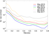 |
Fig. 1 5σ raw contrast of the IFS images at all epochs but March 2016. |
2.2 IRDIFS and IRDIFS_EXT data reduction
We performed the basic data reduction of IRDIS and IFS (bad pixel removal, flat fielding, image alignment, sky subtraction) with version 0.15.0 of SPHERE Data Reduction and Handling (DRH) pipeline (Pavlov et al. 2008). Further elaboration of the images (deconvolution for lenslet-to-lenslet cross talk, refinement of the wavelength calibration, correction for distortion, fine centring of the images, frame selection) was performed at the SPHERE Data Center (DC) in Grenoble1 (Delorme et al. 2017). Additional details on the adopted procedures are described in Zurlo et al. (2014), Mesa et al. (2015) and Maire et al. (2016). We then applied various algorithms for differential imaging such as classical ADI (cADI; Marois et al. 2006), template-LOCI (TLOCI; Marois et al. 2014), and principal component analysis (PCA; Soummer et al. 2012; Amara & Quanz 2012). These procedures are available at the SPHERE DC through the SpeCal software (Galicher et al. 2018).
For IFS, the cADI is based on a median combination of the images, while the PCA is evaluated on the whole image at the same time; no exclusion zones are considered.
For IRDIS, no spatial filtering was applied to the data beforehand. We performed several reductions and verified that both disk and wide companions (see Appendix A) are detected using the alternate methods. We also confirm that these detections are robust across a range of algorithm parameter space. In classical ADI, SpeCal averages the cube of frames over the angular dimension for each spectral channel to remove the speckle contamination. After a rotation is applied, the frames are averaged using mean or median combination to produce one final image per spectral channel. The median-combination is applied for disk images because it is less sensitive to uncorrected hot/bad pixels. When estimating the photometry of the candidate companion the mean is used instead of the median to preserve linearity. Principle components analysis is evaluated on the whole image at the same time; no exclusion zones are considered and the number of PCA modes range from 2 to 5. There is no frame selection to minimise the self-subtraction of point-likesources when deriving the principal components. The principal components are calculated for each spectral channel independently. Each frame is then projected onto the first two to five components to estimate the speckle contamination. For TLOCI reduction, the minimum residual flux of a putative companion, because of self subtraction, is at least 15% of the candidate flux. The minimum radius where the speckles are calibrated and subtracted is 1.5 FWHM using annular sections. The maximum number of frames to estimate the speckles is 80 and no singular value decomposition cutoff was used. The speckle contamination is estimated by linear combination of frames that minimizes the residual energy in the considered region using the bounded variables least-squares algorithm by Lawson & Hanson (1974). The contrast curves calculation assumes a flat spectra for the companion candidates.
Although Spectral Software can perform spectral differential imaging (SDI; Racine et al. 1999), we use procedures that treat each individual spectral channel separately. We also performed Reference Star Differential Imaging (RDI), subtracting from each datacube frame a reference PSF. This PSF is that of the most similar star (in terms of luminosity and noise model) observed during the same or a close night, with the same setup used for our target. HD 95086 is ideal for our purpose since the debris disk and close companion around this star are faint (Chauvin et al. 2018) and do not impact on the photometry of HD 100546. The RDI was performed using as reference the observations of HD 95086 taken on May 3, 2015.
In addition, we used a set of customised data analysis procedures set up for performing the monochromatic PCA, taking into account the effect of the self-subtraction.
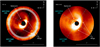 |
Fig. 2 May 2015 IFS collapsed YH (left panel) and IRDIS K1K2 (right panel) results for HD100546 using RDI. Both images are r2 -scaled to also enhance structures at larger radii. The grey circle in the left panel indicates the SPHERE AO control radius at r ≈ 20 ×λ∕D. |
2.3 IRDIS PDI data reduction
In IRDIS PDI observations, the stellar light is split into two beams with perpendicular polarization states. A half-wave plate allows to shift the orientation of the polarization four times by 22.5° in order to obtain a full set of polarimetric Stokes vectors. The data presented in this work are reduced following the double difference method (Kuhn et al. 2001) as described by Ginski et al. (2016). The resulting Q and U parameters are finally combined to obtain the polar Stokes vector Qϕ and Uϕ as from
 (1)
(1)
 (2)
(2)
where ϕ is the position angle of the location of interest (Schmid et al. 2006). With these definitions, positive Qϕ values correspond to azimuthally polarised light, while negative signal is radially polarised light. Uϕ contains all signal with 45° offset from radial or azimuthal.
3 The disk
3.1 Disk morphology
3.1.1 Intensity images
Figure 2 shows the central part of the HD 100546 disk as obtained applying the RDI technique both for IFS and IRDIS. The light distribution appears elliptical, oriented in agreement with PA = 146° and the ratio between major and minor axis is consistent with an inclination of 42° as found by Ardila et al. (2007) using HST/ACS observations of HD 100546. The southeast (SE) part in both images appears brighter than the northwest (NW) part. The southwest (SW) part of the disk along the minor axis represents the near side to the observer and shows a strong depletion in the light distribution at a separation of > 0.2′′. The two wings detected in the H2H3 and K1K2 bands by Garufi et al. (2016) are also distinguishable at IFS shorter wavelengths, especially the northern one. Hereafter, we use Garufi et al. (2016) nomenclature for these two structures since they appear symmetric with respect to the minor axis, and do not have the same concavity, as expected in the case of disks with multiple spirals. In these images we do not detect the spiral arm seen by Avenhaus et al. (2014), but in the IRDIS K1K2 data there is a thin spiral-arm-like structure, almost circular, at a separation of 0.2′′ from PA ~ 100° to ~ 4°, that is barely visible also in the IFS images. No relevant features are detected at separations greater than ~ 0.8′′ in both these images, so they are masked. The bright ring seen in IFS data at a separation of 0.65′′ corresponds to the SPHERE AO control radius2. The control radius at the wavelengths of IRDIS K1K2 bands is at a separation of 1.1′′, therefore not visible in Fig 2.
Figure 3 shows the results of the cADI analysis of the SHINE observations of HD 100546, where several disk structures are easily visible.
In the first row, we report for the first time SPHERE/IFS images of the disk-bearing HD 100546. YJ collapsed image (Fig. 3a) shows the two wings described in Garufi et al. (2016) with a higher angular resolution that allows for detection of an additional curved structure in the NW side, between 284° and 350°, at a separation of about 0.3′′ and a southern spot. The IFS also recovered the SE fainter arm and the IFS YH collapsed image (see Fig. 3b) reveals a single wider northern wing that barely reaches the expected position of CCb. The prominent southern wing extends up to 0.7′′ and PA = 90°. Two additional spiral-arm-like features are also clearly visible. Referring to Follette et al. (2017), who provide a clear description of the innermost structure of HD 100546, these two arms may be identified with “S4” and “S6”; the southern one corresponds to the SE arm. In our image, an additional arm that lies above the southern wing, and starts from it, seems to extend to the east up to ~0.6′′ and PA = 90° (eastern arm in Fig. 3b) and can be properly reproduced with a logarithmic spiral with a large pitch angle (~ 50°). There is also a hint of the “S2” spiral structure observed by Follette et al. (2017), east of the northern wing. No bright PSF-like knots are recovered along the arms at these wavelengths. We confirm the presence of a dark area just offset from the wings in the west direction, up to ~ 0.3′′, also detected in the RDI, where the disk shape is less altered thanks to a negligible self subtraction. This dark area is also present in the IFS YJ images where it looks less deep. In Fig. 3c the non-coronagraphic YH collapsed image clearly reveals the two bright wings and the SE arm and it appears clear that the distribution of light is uninterrupted between the wings, with only a smalldepletion along the minor axis that is likely an artifact of the ADI analysis: the two wings appear then as a unique structure, symmetric to the minor axis, whose central part lies very close to the star. The darker area in the west is still visible.
In the bottom row of Fig. 3 we present IRDIS TLOCI images. In Fig. 3d and e, we show the median H2H3 and K1K2 images, respectively. The two wings, the SE arm, the east arm and the dark area appear clearly visible in both images, but show some differences with respect to shorter wavelengths. A diffuse signal is visible on the top of the northern wing in H2H3 and also in K1K2, but is less luminous. This is located close to the expected position for CCb (Quanz et al. 2015; Currie et al. 2015). The east arm extends up to r = 0.7′′ and PA = 64° in the H2H3 filter pair but only to r ~ 0.4′′ and PA ~ 90° in K1K2. In the H2H3 image, a second dark area is visible to the west side starting at ~ 0.6′′ until ~ 0.9′′. At larger separations, at least two spiral arms are visible in the south, ranging from ~ 1.1′′ to ~ 2.3′′.
We notice that the SPHERE data were obtained under worse seeing conditions than those recorded when using GPI. The greatest difference in the disk structures concerns the dimension of the “S4” spiral (Follette et al. 2017) which looks more extended in the GPI observations than in the SPHERE data. Moreover, a few differences between GPI and SPHERE observations can be noted on the extended structures around the location of the candidate companion CCb. This is discussed further in Sect. 4.
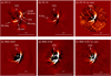 |
Fig. 3 ADI images obtained for HD 100546. Top panels: IFS cADI images. Panel a: YJ from June 2015; Panel b: YH from May 2015; Panel c: JH no coronagraphic image from April 2016. Bottom panels: IRDIS TLOCI images. Panel d: H2H3 from June 2015; Panel e: K1K2 from May 2015; Panel f: K1K2 no coronographic image from Feb 2017. In all the images north is up, east is left. |
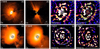 |
Fig. 4 Polarised light images of HD100546 from SPHERE/IRDIS. Panel a: the Qϕ image in the J band. Panel b: the Uϕ image in the J band. Panel c: unsharp masking of the Qϕ image in the J band (see text). The inner box defines the region displayed in the bottom row. Panel d: labelled version of panel c. The inner inset circle is from panel g. Panel e: inner detail of the Qϕ image in the J band. Panel f: inner detail of the Qϕ image in the K band. Panel g: unsharp masking (see text) of panel e. The grey circle indicates the IRDIS control radius at r ≈ 20 × λ∕D (see text). Panel h: unsharp masking (see text) of panel f. Features visible from both panels g and h are labelled. The purple dot indicates the location of CCb from Quanz et al. (2013). In all images, the central star is in the middle of the grey circle, symbolizing the instrument coronagraphic mask. The logarithmic colour stretch is relatively arbitrary and refers to positive values, except in panels a and b where it is the same. North is up, east is left. |
3.1.2 Polarimetric images
The polarimetric images resulting from the data reduction described in Sect. 2.3 are shown in Fig. 4. We found that the outer disk (> 1′′) is well imaged in the short exposure in the J band. The K-band image, however, is affected by thermal background in the detector, which prevents us from obtaining similarly good images at larger radii.
The Qϕ image of the whole system is shown in Fig. 4a, whereas the respective Uϕ is shown in Fig. 4b. Strong signal is detected from both images. In particular, the Uϕ image shows positive values to the north and south and negative values to the east and west. Four prominent stellar spikes are left from the data reduction in both images. A possible explanation for these artifacts is related to the bright (J = 6.42 mag) central star polarization degree which leads to the spikes being imperfectly cancelled throughout the process of subtraction of the beams with different polarization states. There is indeed a compact polarised inner ring (0.24–0.7 au; Panić et al. 2014, unresolved from the star in our images) that can contribute, even if the NIR excess originating from that region is not particularly large for this source and this effect is not appreciable in other stars with similar sub-au disks.
The circumstellar disk is clearly visible in Fig. 4a. To image a larger flux range, the images are shown in logarithmic scale. In the image, a number of wrapped arms at radii 1.5′′ –3′′ from the central star are visible at all azimuthal angles. In particular, we recover the arms to the south imaged by Boccaletti et al. (2013) and Garufi et al. (2016) and those to the north visible from the Hubble Space Telescope (HST) image by Ardila et al. (2007).
To highlight elusive disk features from Fig. 4a, we applied an unsharp masking to the image similarly to what is described by Garufi et al. (2016). This technique consists in subtracting a smoothed version of the original image from the image itself. The result of the unsharp masking, obtained by smoothing Fig. 4a by approximately times the angular resolution of the observations, is shown in Fig. 4c. Looking at this image, it is possible that the majority of the structures visible from Fig. 4a are part of a unique arm which is wrapping for at least 540°, as indicated by the green line in Fig. 4d and as already noticed by Garufi et al. (2017). Another bright arm visible to the south seems to have a similar origin but is seen to extend eastward with a larger aperture angle (see the cyan line of Fig. 4d).
In the inner zone of the disk, inside ~ 1′′, the polarised flux is dramatically higher, even though two regions with reduced flux (appearing black in the image) are visible at PA ~ 160° and PA ~ 300° (Fig. 4a), similarly to what was found by Quanz et al. (2011) and Avenhaus et al. (2014).
Figure 4e and f show the zoomed Qϕ image in J and K bands of theinnermost disk region. Two bright lobes are visible to the SE and to the NW, with the former being brighter than the latter. Inward of these lobes, the disk cavity is marginally visible just outside of the instrument coronagraphic mask. Similar to Fig. 4a, disk features are not easily recognisable. Therefore, we also apply an unsharp masking to these images, with smoothing by approximately six times the FWHM, which results in Fig. 4g and h. In both images, a number of possible features are visible. Among them, we only give credit to those that are persistent across unsharp masking procedures (i.e. by varying the smoothing factor) and, more importantly, across wavebands. Features that are radially distributed at r ≈ 20 × λ∕D (~ 60 au) are masked out in Fig. 4g, because this region corresponds to the SPHERE control radius (see Fig. 4g). Features present in both the J and K band images are labelled in red in Fig. 4h. The morphology of the identified structures resembles the shape of the arms at larger radii and is consistent with the known disk geometry. The innermost of these features was also detected by Avenhaus et al. (2014) and Garufi et al. (2016), whereas the others were not. Interestingly, the location of CCb, as defined by Quanz et al. (2013), is very close to one of these arm-like structures. From this data set, we cannot infer whether a spatial connection between the inner arms (in red) and the outer arm (in green) exists.
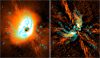 |
Fig. 5 IRDISPDI J band Qϕ image (left panel) and the results of a simulated cADI analysis on this image. Overplotted in cyan are the isophotes of IRDIS cADI H2 observations. |
3.2 Comparison between ADI and PDI
While the southern spiral arms of the outer disk (> 1′′) in the IRDIS H and K images are well detected also in the IRDIS PDI J (Figs. 3d and e, and 4a), the central part of the PDI data do not show any axis-asymmetric structure. Using the unsharp masking technique on PDI data, we found three spiral arms in the innermost region (Fig. 4h) that have no counterpart in the intensity image. To compare ADI results with the PDI ones, we then performed pseudo-ADI on the IRDIS DPI J-band images as follows: we used the parallactic angle values of the three different IRDIFS_EXT observations to simulate a simple cADI analysis based on the IRDIS DPI image. The results are given in Fig. 5: the simulation generates an image that is in better agreement with the IRDIS cADI images. On the other hand, PDI images are directly comparable with RDI images. These two methods allow us to better study the light distribution in the disk without self-subtraction effects.
3.3 Disk spectrum
In general, disk flux in the NIR is dominated by scattered light, while the brightness of a young planet is dominated by thermal emission. Therefore, to distinguish between a self shining planet and the disk we studied the total spectrum of the HD 100546 disk. Previous attempts to derive the spectrum of the disk of HD 100546 were done by Mulders et al. (2013) using HST data, and by Stolker et al. (2016) using data from NACO at VLT.
In order to derive the disk spectrum, we estimated the ratio between the total disk flux and the stellar one. We used the RDI datacube obtained with IFS in May 2015, where self subtraction is less aggressive. The target to reference intensity ratio is measured ina specific region of the image, defined as the pixels of the wavelength-combined RDI image with a value above a determined threshold. This procedure yielded an elliptical region with a deprojected radius of ~ 40 au, without the central region that corresponds to the coronagraph, as shown in the small inset in Fig. 6. An adequately rescaled mask, in order to sample the same area of the disk, was also applied to the IRDIS RDI frames.Several reference stars were tested to confirm that the choice of the HD 100546 data set and the reference star do not affect the final contrast spectrum (all data sets considered have correlation coefficient > 0.98 with that of HD 100546).
The relative flux spectrum is shown in Fig. 6. Since we are interested in the disk albedo, the flux calibration of the disk is based on broadband photometry. The uncertainties on each wavelength (blue bars) were estimated as the standard deviation of the mean of the spectra for individual pixels. Moreover, we also show the intensity 1σ range over the population of individual pixels (light blue area). The regions between 1.08–1.15 μm and 1.35–1.48 μm are affected by strong water absorption due to the Earth’s atmosphere that cannot be perfectly recovered during the RDI process and were therefore removed.
The difference in contrast magnitude is close to zero between H and K bands (K–H ~ 0.03, in agreement with similar analysis presented by Avenhaus et al. 2014 exploiting NACO H, Ks and L′ filters), and the spectrum appears featureless, with the disk reflecting about 8% the stellar light in the Y band and about 11% in K band. This is very similar to the spectrum obtained by Mulders et al. (2013). We tried to represent this spectral distribution assuming light reflected by dust with a constant albedo. Mulders et al. (2013) suggested that in the NIR regime, light scattered off the HD 100546 outer disk surface is not only scattered stellar light, but the contribution of the light reprocessed by the inner disk (0.24–0.7 au; Panić et al. 2014) is not negligible. Therefore, we took into account a possible reddening due to the presence of the inner disk that can absorb stellar light, done following Cardelli et al. (1989). The free parameters are subsequently reddening and the (total) disk reflectivity. The first is related via extinction (AV) and reddening (RV) to the slope of the spectrum, the latter is the combination of the albedo and the disk-emitting area defined above3. The best solution gives AV = 2.11 and albedo A = 0.96 that is very high and not credible. An alternative more palatable explanation is that the albedo of dust is not constant with wavelength. A similar explanation was already suggested by Mulders et al. (2013) and Stolker et al. (2016). A variation of the scattering efficiency from 0.43 at 1 μm up to 0.63 in the K-band may explain the observations. This points towards relatively large particle sizes.
The reddened spectrum we derive was also seen in HD 100546 HST data and was explained by the effect of forward scattering of micron-sized particles (Mulders et al. 2013). Further analysis based on the PDI data confirmed the presence of these particles, determining the phase function (Stolker et al. 2016).
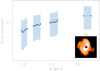 |
Fig. 6 Disk mean spectrum of HD 100546 along the wings. The blue dots and the shaded regions refer to the median value and its 3σ uncertainty. The green line represent the best fit obtained with light reflected by dust with constant albedo A = 0.65. In the bottom-right inset panel, the area selected for the spectrum extraction on the RDI images is delimited in blue. |
3.4 Disk geometrical model
The disk structure of HD 100546 has been investigated in different wavelength regimes. ALMA observations suggest that the millimetre-sized grains are located in two rings: a compact ring centred at 26 au with a width of 21 au, and an outer ring centred at 190 ± 3 au with a width of 75 ± 3 au (Walsh et al. 2014). The same two-ring structure was suggested by Panić et al. (2014), who used MIDI/VLTI data to probe micron-sized grains. They also came to the conclusion that there is an additional inner disk that extends no farther than 0.7 au from the star. The gap is about 10 au wide and free of detectable MIR emission. Much larger dust, rocks, and planetesimals are not efficient H-band emitters, and our data do not exclude their presence inside this gap. Analysis of the SED of HD 100546 shows that the radial extent of the gas is ~ 400 au (e.g. Benisty et al. 2010). The presence of an extended disk is clearly indicated also by scattered light, NIR, and sub-millimetre imaging (Pantin et al. 2000; Ardila et al. 2007; Quanz et al. 2013; Avenhaus et al. 2014; Currie et al. 2014; Garufi et al. 2016; Follette et al. 2017).
To constrain some of the HD 100546 disk properties we built a simple geometrical model based on analytic functions that can describe theinner part of the system between 10 and 200 au. This model is similar to that described by Stolker et al. (2016). The basic assumption of this model is that the disk photometry can be described by light scattering on a single surface. In our model, the scattering function for total intensity images is described by a two-component Henyey–Greenstein (HG) function (Henyey & Greenstein 1941) with coefficients as defined in Milli et al. (2017) for HR 4796. For PDI data we used the function given by Stolker et al. (2016), cf. Eq. (8). The light from the star is reflected by the optically thick disk surface, that lies above the disk midplane as described by the power law:
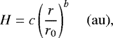 (3)
(3)
where r0 corresponds to 1 au and c is in astronomical units. Gaps present in the disk are modelled by decreasing the disk height H to 0 au. This does not mean that the gaps are really empty, but simply that we cannot model emission from these regions with our approximation. Assuming the disk geometry as found from the MIDI data, which trace micron-sized grains, and the ALMA data, which trace millimetre-sized grains, we have also assumed the same disk geometry for the scattered light traced by SPHERE, being aware that different wavelengths probe of course grains of different sizes and that grains of different sizes may occupy different physical locations in the disk. Therefore, we set the rings range between ~10 and ~40 au (hereafter ring 1) and then from ~150 to ~230 au (hereafter ring 2).
The thin inner ring (hereafter ring 0) extending between 0.24 and 0.7 au is behind the SPHERE coronagraph and therefore is not included. The positions of the inner and the outer edge of the ring 1 are well constrained by the observed radial profiles: the inner edge must be at least partly behind the coronagraph, otherwise the disk wall will be clearly visible on the semi-minor axis radial profile on our images, while the outer edge is visible on the semi-major axis. The flaring parameter b is derived by the flux ratio between the peak of the near and the far side of the semi minor axis while the scale factor c impacts the shadowing effect of the disk.
We first compared our model to RDI images; we did it for IFS and applied the same model also to IRDIS. We found out that a disk with b = 1.08 and c = 0.13 best reproduces the HD 100546 radial profiles (Fig. 7), quite similar to the τ = 1 disk surface for H and K band derived by Stolker et al. (2016). The disk rings 1 and 2 extend between ~ 12 and ~ 44 au and between ~110 and 250 au, respectively, consistent with previous results based on ALMA observations (e.g. Walsh et al. 2014). The model for the outer disk is however fainter than observed, suggesting a larger flaring at large separations, though it should be considered that the RDI images are not very accurate at very high contrast levels. However, this model is also in quite good agreement with the IRDIS PDI images in broad J band as shown in Fig. 8. We notice that the inner edge of ring 2 and the outer edge of ring 1 might correspond to resonances 3:2 and 1:2 with a hypothetical massive object located at an orbit of 70 au in radius, which is not far from the observed location of CCb (see following section).
The resulting RDI images are shown in Fig. 9. The residuals clearly show the presence of the two wings, that are even more evident when applying the ADI method to this model. To show this, we constructed a data cube (x, y, lambda, time) made of the sum of the disk model and of the reference image used in our RDI analysis, that is, the data set of HD 95086. This datacube was then processed by the same ADI routine used for the original HD 100546 datacube. In this case, the two bright wings visible in all the images in Fig. 3 can only be reproduced by assuming a much thicker disk, with a value of H ~ 30 au at r ~ 40 au. This is because the bright wings visible in the ADI images, which correspond to the edge of the disk, are described by an ellipse whose centre is far from the star.
A similar result has been found for several disks, a classical example being HD 97048 (Ginski et al. 2016). As explained in their Fig. 5, disk images that may be described by off-centre ellipses indicate the presence of material located well above the disk mid-plane. This was also demonstrated by recent hydrodynamical simulations performed by Dong et al. (2016) coupled with simple radiative transfer models. These simulations demonstrate that a giant planet can open a gap in a disk creating a ring that, when seen at an intermediate viewing angle, and reinforced by the ADI process as explained above, appears as two pseudo-arms placed symmetrically around the minor axis winding in opposite directions. They conclude that these simulations can describe HD 100546 as well. They also predicted the presence of a “dark lane” parallel to these disk pseudo-arms that is due to the self shadowing by the disk. In the case of HD 100546, the elliptical light distribution may indicate the presence of a ring of material at ~40 au, close to the outer edge of the intermediate disk, but at a height of ~ 30 au on the disk plane. This is about four times the value obtained with Eq. (2), using the best value we obtained for b and c. The origin of this ring is not clear; we reiterate however that the edge of the intermediate disk can be explained by a 2:1 resonance with a hypothetical massive object located at about 70 au.
In order to agree with PDI and RDI data, we have to assume that this material is optically thin, contributing only marginally to the total emission from the disk. However, the higher (about a factor 25) sensitivity provided by ADI allows its detection.
We note that a multi-ring configuration similar to that observed in HD 100546 is also seen around other objects. We mention in particular HD 141569A, where rings and outer spiral arms were observed with HST in the visible (Augereau et al. 1999; Mouillet et al. 2001; Clampin et al. 2003), and the NIR with NICI (Biller et al. 2015; Mazoyer et al. 2016) and SPHERE (Perrot et al. 2016). Moreover, the face-on disk surrounding TW Hya (van Boekel et al. 2017) presents three rings and three gaps within ~2′′ of the central star. These features were identified using optical and NIR scattered light surface-brightness distribution observed with SPHERE. Multiple rings were also observed in the inclined system RX J1615.3-3255 (de Boer et al. 2016) combining both visible polarimetric images from ZIMPOL with IRDIS and IFS in scattered light.
Finally, we notice that a planet sculpting a cavity is not a unique explanation for the gaps. In addition some models with planets located outside of the gap can reproduce the gaps, or a single planet can open multiple gaps under particular circumstances (Dong et al. 2017).
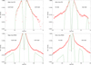 |
Fig. 7 Radial profile along the semi-major and semi-minor axes of HD 100546 RDI images (red dots) compared with the best-fit model (green line) obtained for IFS and IRDIS. |
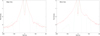 |
Fig. 8 Radial profile along the semi-major and semi-minor axes of HD 100546 PDI images (continuum line) compared with the best-fit model (dashed line) IRDIS. |
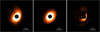 |
Fig. 9 From left to right: IFS RDI image, model and residuals. Image are displayed with the same linear colour bar from 6 × 10⁻³ to 1 dex. North is up, east is left. |
4 The candidate planets
4.1 Detection limits
Two candidate companions around HD 100546 have been proposed over the years (Quanz et al. 2013, 2015; Brittain et al. 2014; Currie et al. 2015). We investigated IFS and IRDIS images to find signatures of the already proposed candidate companions or new signatures. None of the IFS images shows evidence of new candidate companions above detection threshold. while in the IRDIS images seven objects were identified as background stars (see Appendix A).
To properly discuss our data, we should consider the detection limits we used for point sources. The IRDIS 5σ detection limits for point sources were obtained through the SpeCal software (Galicher et al. 2018); it estimates the noise level σ as the azimuthal standard deviation of the flux in the reduced image inside annuli of two times FWHM in width at increasing separations, and rescales it as a function of the stellar flux derived from the off-axis PSF images, taking into account the transmission of the neutral density filter used to avoid the star image saturation. We evaluated the IFS 5σ contrast limits in the PCA imagesfollowing the method described in Mesa et al. (2015). In summary, the algorithm determines for each pixel the standard deviation of the flux in a 1.5 × 1.5λ∕D box, centredon the pixel itself and divides it by the proper stellar flux (as described above). For a given separation, the 5σ is then computed as five times the standard deviation of the values obtained for all the pixels at that separation. Finally, both IRDIS and IFS 5σ values are corrected for the algorithm throughput and for the small number statistics (Mawet et al. 2014). To this purpose, fake companions, ten times more luminous than the noise residuals in the final reduced image, were injected in the pre-processed frames at various separations from the star and the datacube is reduced as before. This is then repeated at several different position angles and the throughput final value is the average of fake planets flux depletion at the same distance, corrected for the coronagraph attenuation.
In Fig. 10 (top panel), we show the deepest 5σ contrast curves obtained with IRDIS and IFS for HD 100546 in the H band. The TLOCI-based analysis shows that IRDIS could reach a 5σ contrast >12 mag at separation > 0.5′′ and even 15 mag at separations of 1.5′′ in both H2 and H3 bands. The deepest IFS contrast is reached when applying SDI and PCA. However, all these approaches, widely used for isolated point-like sources, likely underestimate the contrast limits in the presence of a bright disk such as that of HD 100546, because the disk flux enters both in the estimation of the background and in the attenuation effect and therefore a less aggressive approach (e.g. monochromatic PCA with low number of modes) is more suitable. We considered the HD 95086 data set mentioned above to demonstrate the expected contrast limit in absence of the disk (red dash-dotted line in Fig. 10). In this figure, we also show the H magnitudes of the two candidate companions around HD 100546 from Currie et al. (2015) using GPI. The impact of the disk on the contrast limit for IFS images is not negligible at separations of both CCc (~ 2.2 mag) and CCb (~1.5 mag). We note here that CCc with a contrast of 7.12 mag should be nominally visible in the IFS May 2015 and May 2016 datasets, where the contrast limits at the candidate separation are 7.3 and 7.8 mag, respectively. The CCb (Δ H = 13.44, r ~0.47′′), instead, is below the detection limit in the H band. However, it would be above the detection limit if we were to consider the limits applicable to a star without a luminous disk.
4.2 The candidate companion c
No obvious point-like structure is visible at the expected position of CCc in any of our IFS and IRDIS data sets in all epochs. Using a different reduction approach, Garufi et al. (2016) identified a bright knot in the SE arm (r ~ 0.120 ± 0.016′′, PA ~ 165±6°) at least in the H band for theMay 2015 data. On one hand, one could try to associate CCc with this knot, as it may lie at or just inside the disk cavity and is counterclockwise from the position noted by Currie et al. (2015), as expected for an orbiting object predicted from Brittain et al. (2013). On the other hand, these results do not establish CCc as a companion since there are equally compelling alternatives.We detect bright, elongated emission at a similar location in all of our IFS and IRDIS H2H3 data sets, suggesting confusion between bright disk emission and that of any point source. Moreover, all our data sets have a light distribution along the two wings that is nearly symmetric around the disk semi-minor axis, with the NW side being more luminous, as already found by Follette et al. (2017). The emission could simply be a non-polarised hot spot in the disk. Furthermore, this structure is detected at locations compatible with a stationary object with respect to the star, despite the fact that a planet orbiting the star on the disk plane as detected by Brittain et al. (2014) should move by ~ 15° (one resolution element at that separation) during our campaign; the feature is clearly visible only when using non-aggressive reduction methods, such as monochromatic PCA with only one component.
A key challenge in interpreting these data is the effect of processing. At CCc’s angular separation, parallactic angle motion is small (1.2λ∕D for our data) and self-subtraction due to processing is severe. Processing could anneal the disk wings to look like a point source (a shock, a convergence of spiral features, etc.). Alternatively, processing might preferentially anneal a point source, making it appear radially elongated and indistinguishable from the disk wings. Additionally, the proximity of CCc to the coronagraph edge when a mask was used might affect both GPI and SPHERE results. With the coronagraph removed, the brightest part of both southern and northern wings shifts closer to the minor axis (Fig. 11). The SPHERE coronagraph we used, indeed, is 0.03′′ smaller than that used in GPI H-band observationsand this technical difference could explain the difference in the results obtained with the two instruments. Finally, we should consider that the observation taken by Currie et al. (2015) is not simultaneous to IFS and IRDIS observations and that the sky conditions were better. This leaves open the additional possibility that we could not recover the same feature detected by Currie et al. (2015) because the orbital motion moved it behind the coronagraph or the circumstellar disk during this interval of time.
Investigating the nature of the claimed CCc further requires a detailed forward-model of both the point sources and the disk over multiple data sets, taking into account the impact of the coronagraphs, which is beyond the scope of this paper.
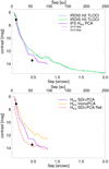 |
Fig. 10 Top panel: contrast curves for HD 100546 obtained in the HIFS band for the two best IFS datasets applying SDI+PCA and for IRDIS H2H3 dataset applying TLOCI. Bottom panel: The IFS May 2015 contrast curve shown above is compared with the result obtained with a two-mode monochromatic PCA (orange curve) and with the contrast curve in the HIFS band for HD 95086 applying SDI+PCA (in red dashed-dotted line). The planets contrast values measured in the H band obtained by Currie et al. (2015) with GPI are reported in both panels. |
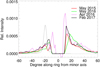 |
Fig. 11 Intensity profile as a function of phase of the two wings at different epochs. Phase 0 corresponds to the near side of the semi-minor axis and negative values correspond to the SE wing. The dashed profile corresponds to a point-like source located at the expected position of CCc crossing the ring with the contrast upper limit given by Currie et al. (2015). The April 2016 data set was scaled by an arbitrary factor of 1.6 to overlap other profiles. |
4.3 The candidate companion CCb
Since the initial discovery of HD100546 b by Quanz et al. (2013), its re-detection has been reported by different groups using different instruments and in multiple wavelengths (Quanz et al. 2013, 2015; Currie et al. 2014). However, the debate over the nature of CCb was recently reactivated by the results obtained by Currie et al. (2015) and Rameau et al. (2017), both with GPI H-band observations. In both cases, a clear signal is detected at a location possibly compatible with CCb, but, on one hand, Currie et al. (2015, 2017) identified this with CCb (a point source superimposed on a flat disk component), and on the other hand, Rameau et al. (2017) interpreted it as stellar scattered light, being point-like or extended depending on the processing method used.
In the following discussion we use a non-aggressive monochromatic PCA approach with only one component over the whole IFS field of view simultaneously, and over the inner circle of 0.8′′ for IRDIS one. Moreover, we exploit the very wide spectral range simultaneously offered by the SPHERE IRDIFS_EXT setup (from 0.95 up to 2.2 μm). All IRDIS K1K2 datasets show a clear diffuse emission on top of the northern wing (as already noticed by Garufi et al. 2016 for the 2015 datasets) that is compatible with the CCb detections in L′ and M bands using NACO.
In order to obtain a more precise characterisation of this feature, we focused on the two best IRDIFS_EXT datasets and found that the position of this source varies a little between the two epochs, as shown in Table 2. From the disk velocity retrieved from spectroastrometric analysis of different molecules (see e.g. Acke & van den Ancker 2006; Panić et al. 2010; Brittain et al. 2009) and with ALMA observations (Walsh et al. 2014), it was derived that the disk rotates counterclockwise, with the SW part being the closest to the observers. We discover that the feature we detect is moving counterclockwise and its astrometry, combined with previous detections, is compatible with a Keplerian motion on the disk plane. This is shown in Fig. 12, where we present the run of the separation and position angle of this source with time, using data from Quanz et al. (2013, 2015) and Currie et al. (2014) and the two best K1K2 epochs from SPHERE. We adopted the disk plane inclination of 42° and position angle of 146° (Pineda et al. 2014), obtaining an orbital radius of 545 ± 15 mas that corresponds to 59.5 ± 2 AU at the distance of HD 100546. Given the stellar mass of 2.4 M⊙ (see e.g. Quanz et al. 2013), the corresponding period is 299 yr. We superimposed the predictions for a similar orbit on the run of separation and position angles shown in Fig. 12, dashed lines. The agreement between expectation and observationsis fairly good, in view of the relatively large error bars associated with all these data. We conclude that the motion of CCb is compatible with a circular orbit on the plane of the disk, in the same direction as the disk rotation, although there is room for different orbital solutions and also a scenario whereby the object is stationary, given the uncertainties on the positions. If this orbital solution is correct, we could therefore predict that in Spring 2019 CCb will have moved enough to disentangle the motion from being a stationary object, or it will disappear behind a disk structure. For example, assuming a nominal co-planar, circular orbit at 59.5 au, CCb should appear at a separation of ~ 440 mas and PA ~ 17° in May 2019, which is roughly three resolution elements away from its position in May 2015. However, the astrometric points hint at a slower motion, which could be due to an eccentric and/or non-coplanar orbit, and would mean that an even longer time period is needed to confirm the CCb movement.
This object has a contrast of 12.08 ± 0.49 mag in K1 and 11.68 ± 0.60 mag in K2, compatible with the NACO non-detection by Boccaletti et al. (2013), while its H band upper limit is 13.75 ± 0.05 mag. On the other hand, the IRDIS H2H3 data set and the H part of the IFS images (simultaneous to the K1K2 IRDIS data sets) show a diffuse emission, located ~70 mas NW with respect to the previous one in continuation with the northern wing, as shown in Fig. 13. This emission, with median position r = 477 ± 12 mas and PA = 7.2 ± 1.5°, is consistent with the detection in the H-band by Currie et al. (2015) and Rameau et al. (2017). This source is clearly distinct from that detected at longer wavelengths, and appears extended. However, given the angular resolution of GPI and the different H-band filter used in GPI and SPHERE, the detection of Currie et al. (2015, 2017), intermediate between the H and K detections with SPHERE, can be interpreted as a combination of these two. Finally, only very weak diffuse emission was visible at wavelengths shorter than 1.1 μm.
Additional information on CCb cannot be retrieved by the polarimetric data: no emission is seen in the IRDIS Qϕ images as shown in Fig. 4h, while in the PDI+ADI image the residuals due to the telescope spider are not negligible and fall at the location of CCb, meaning that it is impossible to tell whether or not a disk structure at that location could be interpreted as a point source after filtering by ADI.
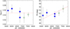 |
Fig. 12 Run of deprojected separation (left panel) and of position angle (right panel) of CCb with time. Data are from Quanz et al. (2013, 2015; blue dots), Currie et al. (2014) and this paper (open diamonds). Dashed lines are predictions for a circular orbit on the plane of the disk. |
Astrometry of CCb in the SPHERE K band at different epochs.
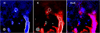 |
Fig. 13 Comparison of HD 100546 images in different band filters. One-component PCA images of IRDIS H2H3 taken on May 29, 2015 (left panel), K1K2 taken on May 3, 2015 (middle panel), and their combination (right panel). Contours refer to IRDIS H2H3. The cross represents Currie et al. (2015) detection in GPI H band, the arrow in the central panel indicates the motion of CCb between the Quanz et al. (2015) detection in NACO L′ band and our May 2016 K1K2 detection of CCb. The grey circle represents the resolution element of the images. |
4.4 Interpreting CCb as an extended source
Previous works suggested that CCb is surrounded by a circumplanetary disk (Quanz et al. 2015; Currie et al. 2015; Rameau et al. 2017). In Quanz et al. (2015), the presence of a spatially unresolved circumplanetary disk (r ~ 1.4 au around a 2MJ object) is considered as an explanation of the discrepancy between the observed values of radius and effective temperature and those obtained by models for very young gas giant planets.
At wavelengths shorter than 2 μm, we evaluated the 5σ limit to the magnitudes of a point source at the presumed location of CCb. With IFS we obtain that it is fainter than the apparent magnitude 19.84 in the J band (1.20–1.30μm), fainter than 19.80 mag in J broad band (1.15–1.35μm), and fainter than 19.05 mag in H; uncertainties on these values came from the noise distribution estimation at the CCb location.
Putting together all the results and the literature ones (see Table 3) we obtain the CCb SED plotted in Fig. 14. Some important arguments that one should take into account while interpreting this SED are as follows. (a) CCb is below detection threshold in our IFS images, so we only estimated the contrast limits in the corresponding area of CCb, while in the H2H3 filter we only detect a very weak diffuse emission at its location. (b) What we see in the IRDIS data at positions corresponding to CCb could be simply a bright structure of the disk. (c) We are not subtracting the disk contribution to the flux. Similar to what is discussed above, the self subtraction on extended sources is not negligible even with this non-aggressive reduction method and it is difficult to estimate because it depends on the specific distribution of light, which cannot be easily modelled. This implies that the ADI technique alters the photometry of the extended object. What we can conclude is simply that the structure seen in our K1K2 images is compatible with an extended object whose apparent magnitude is brighter than what is expected for a point sourceat the same location and is compatible, within the uncertainties, with the flux observed at longer wavelengths.
Given the small difference of contrast between the J/H-band diffuse source and the strong difference with the L/M-band putative point-source, we may represent this emission as the sum of two different sources: a very red compact source and a more extended one with a flatter spectrum. It is clear in fact that this source is redder than the star and cannot be explained as stellar scattered light alone, since a flat contrast (grey line) that fits the short-wavelength points largely fails to reproduce the L and M data. The green line represents the SED of a black body with Teff~ 800 K and no absorption, which implies a radius of the emitting area R = 12.5 RJ. Taking into account the new determination of HD 100546 distance, this result is in fair agreement with Quanz et al. 2015 ( K,
K,  ). It is noteworthy that given the small number of photometric points and limited spectral range, absorption and temperature are degenerate, and therefore many combinations of temperature and reddening can efficiently reproduce the SED. However, given its very young age, the object likely does not emit as a black-body, but the accreting disk shock contribution to the total luminosity is not negligible, and could also be dominant (Mordasini et al. 2017). Also, the filters used are built to provide information on absorbing molecules and therefore can play a role in the flux estimation at given wavelengths.
The luminosity of a forming and accreting planet in different formation scenarios is evaluated in Mordasini et al. (2017). They analysed the case of HD 100546 b in detail, starting from the physical parameters derived by Quanz et al. (2015), and could constrain the mass of this source, albeit with large uncertainties due to different mechanisms allowed. To disentangle the emitting sources and hence estimate the CCb mass, we need to better characterise the SED, which could be possible with space observations with new facilities (like JWST) or with the ELT class instruments. Alternatively, a better spatial resolution will allow us to resolve the circumplanetary region and retrieve the mass of CCb through dynamical models.
The nature of the extended emission detected in the H2H3 filter is not clear. It could either be a source physically bound to CCb, or a bright structure of the disk. Further deep observations and/or a longer (3–4 yr) temporal coverage may help to choose between these possibilities. If we assume that the object is a unique extended source, we obtain that the radius is of the order of r = 34 mas (≃3.7 au), compatible with previous estimations. If this were a circumplanetary disk, the corresponding Hill’s radius (RHill) of the planet would be expected to be about three times larger, following models by e.g. Shabram & Boley (2013), Ayliffe & Bate (2009) and Quillen & Trilling (1998). Therefore, the observed structure is compatible with circumplanetary material around a massive planet that could be responsible for carving the gap as demonstrated by hydrodynamical models (e.g. Pinilla et al. 2015; Dong et al. 2016).
To justify the extended emission, we further consider a spherical cloud around CCb, located at a separation of d = 65 ± 5 au from the star, that reflects stellar light. If its optical depth is τ ≪ 1, then we expect that the total reflected light is c = Aπr2∕(4πd2) where A is the albedo. If A = 0.5 then the expected contrast is c = 4.2 × 10⁻⁴, which corresponds to 8.6 mag, in agreement with our observations. This feature would be unresolved at L and M wavelengths and therefore contributes to the flux of the compact source but should be far less than the contribution due to the companion: its luminosity is compatible within the uncertainties with reflected stellar light from the J to the K band.
We finally note that, in this scenario we are not considering the absorption due to the circumstellar disk material between the star and thecircumplanetary disk. This depends on the thickness of the circumstellar disk and on the height of the planet over the circumstellar disk plane at the epoch of our observations. This effect, and the presence of shadows due to the circumstellar disk that may affect the amount of light incident on a circumplanetary disk, could be not negligible and possibly cause an irregular illumination of the circumplanetary disk. Of course, the true picture could be a combination of all these factors.
We conclude that the origin of this emitting area is still unclear. While its appearance and the SED are compatible with a highly reddened substellar object surrounded by a dust cloud, we cannot exclude other interpretations, such as the superimposition of two spiral arms, the northern wing and the small IRDIS North arm (see Fig. 3), or disk material flowing to a planet due to its perturbation induced on the disk.
Star magnitude m*, the contrast of CCb or its upper limit (cont_b) and the associated uncertainty (err_cont) at different wavelengths.
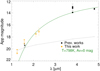 |
Fig. 14 SED of CCb planet and disk combining previous results (black) with our upper limits (orange). The green line represents a black body of 932 K with an absorption AV = 28 mag (seetext). The grey curve represent a grey contrast of 14 mag fitting the short-wavelength observations. In particular, only data corresponding to black filled circles were considered for the relative astrometry. The black star symbol refers to apparent magnitude of a source located at about 28 mas (~ 0.7λ∕D) from the position of the source detected at longer wavelengths, as given by Currie et al. (2015). |
5 Conclusion
We observed HD 100546 with SPHERE using its subsystems IRDIS and IFS in direct imaging and in polarimetry. Our observationsconfirm the presence of a very structured disk and reveal additional features. The different post-processing techniques reveal different characteristics of this complicated disk. RDI and PDI images are dominated by the almost symmetric intermediate and outer disks, while more aggressive differential imaging techniques tell a different story, featuring strongly de-centred rings and spirals. These two views can be reconciled in a picture as follows.
The twobright wings, dominant structures in the IR at separations closer than 500 mas, are a unique structure. This is quite evident from the non-coronagraphic images. The presence of the coronagraph and the use of the ADI technique contributed to cancel out the light in the rings region closest to the star.
The new PDI data confirm the presence of a unique arm warping for 540°. In the innermost regions, three small spiral arms are detected in both J and K bands.
Modelling a geometrical representation of the disk coupled with an analytic scattering function, we obtain that the disk rings 1 and 2 extend between ~15 and ~40 au and between ~110 and 250 au, respectively, consistent with previous results. The inner edge of the ring 2 and the outer edge of the ring 1 correspond to resonances 3:2 and 1:2 with a 70 au radius orbit, suggesting the presence of a massive object located at that separation.
We do not exclude the presence of additional spiral arms inside the disk rings. In particular, we confirm detection of the two possible spiral arms east and south of HD 100546, previously identified by Follette et al. (2017).
The spectrum of this disk does not show obvious evidence for segregation of dust of different sizes and is well explained by micron-sized particles.
Concerning the planets, we have no clear evidence of the CCc as detected by Currie et al. (2015); processing could cause the disk wings to look like a point source or anneal a point source to be indistinguishable from disk emission. This does not exclude that the planet has moved behind the disk in the time between Currie et al. (2015) observations and the time SPHERE data were acquired.
We identify a spatially diffuse source in K band broadly consistent with CCb. When combined with previous measurements, its photometry is consistent with a blackbody-like-emitting source of ~800 K, compatible with a highly reddened massive planet or brown dwarf surrounded by a dust cloud or its circumplanetary disk. The astrometry of this source may have revealed evidence for orbital motion, a result that could be confirmed with future observations. This object could indeed be the disk perturber suggested by the disk modelling. However, other hypotheses are also possible, such as the superimposition of two spiral arms at the location of the L′ and M′ detections.
Acknowledgements
The authors thank the anonymous referee for a very constructive referee report that improved the initial manuscript. The authors thank the ESO Paranal Staff for support for conducting the observations. The authors thank Sascha Quanz, Adriana Pohl and Tomas Stolker for the very useful comments that improved a lot the quality of the paper. E.S., R.G., D.M., S.D. and R.U.C. acknowledge support from the “Progetti Premiali” funding scheme of the Italian Ministry of Education, University, and Research. E.R. is supported by the European Union’s Horizon 2020 research and innovation programme under the Marie Skłodowska-Curie grant agreement No 664931. This work has been supported by the project PRIN-INAF 2016 The Cradle of Life – GENESIS-SKA (General Conditions in Early Planetary Systems for the rise of life with SKA). The authors acknowledgefinancial support from the Programme National de Planétologie (PNP) and the Programme National de Physique Stellaire (PNPS) of CNRS-INSU. This work has also been supported by a grant from the French Labex OSUG@2020 (Investissements d’avenir – ANR10 LABX56). The project is supported by CNRS, by the Agence Nationale de la Recherche (ANR-14-CE33-0018). This work is partly based on data products produced at the SPHERE Data Centre hosted at OSUG/IPAG, Grenoble. We thank P. Delorme and E. Lagadec (SPHERE Data Centre) for their efficient help during the data reduction process. SPHERE is an instrument designed and built by a consortium consisting of IPAG (Grenoble, France), MPIA (Heidelberg, Germany), LAM (Marseille, France), LESIA (Paris, France), Laboratoire Lagrange (Nice, France), INAF Osservatorio Astronomico di Padova (Italy), Observatoire de Genève (Switzerland), ETH Zurich (Switzerland), NOVA (Netherlands), ONERA (France) and ASTRON (Netherlands) in collaboration with ESO. SPHERE was funded by ESO, with additional contributions from CNRS (France), MPIA (Germany), INAF (Italy), FINES (Switzerland) and NOVA (Netherlands). SPHERE also received funding from the European Commission Sixth and Seventh Framework Programmes as part of the Optical Infrared Coordination Network for Astronomy (OPTICON) under grant number RII3-Ct-2004-001566 for FP6 (2004-2008), grant number 226604 for FP7 (2009-2012) and grant number 312430 for FP7 (2013-2016).
Appendix A Background objects in the IRDIS field of view
Separation in α and δ of the background objects in the IRDIS FoV of HD 100546 considering data from 4 May 2015, May 29th 2015 and May 31st 2016.
As described in Sect. 3, seven points sources are detected in the IRDIS field of view. Their astrometry and photometry are listed in Table A.1, and Fig. A.1 unambiguously shows that all of them are background objects.
 |
Fig. A.1 Toppanel: proper motion in α and δ of the background objects in the IRDIS FoV of HD100546 considering data from May 4, 2015 (filled black), May 29, 2015 (open black), May 31, 2016 (filled red). Dotted points and error bars represent the expected position for a background object. Middle panel: observed time variation of the separation compared with the expected one for a background object. Bottom panel: observed time variation of the position angle compared with the expected one for a background object. |
References
- Acke, B., & van den Ancker, M. E. 2006, A&A, 449, 267 [NASA ADS] [CrossRef] [EDP Sciences] [Google Scholar]
- Amara, A., & Quanz, S. P. 2012, MNRAS, 427, 948 [NASA ADS] [CrossRef] [Google Scholar]
- Ardila, D. R., Golimowski, D. A., Krist, J. E., et al. 2007, ApJ, 665, 512 [NASA ADS] [CrossRef] [Google Scholar]
- Augereau, J. C., Lagrange, A. M., Mouillet, D., & Ménard, F. 1999, A&A, 350, L51 [NASA ADS] [Google Scholar]
- Augereau, J. C., Lagrange, A. M., Mouillet, D., & Ménard, F. 2001, A&A, 365, 78 [NASA ADS] [CrossRef] [EDP Sciences] [Google Scholar]
- Avenhaus, H., Quanz, S. P., Meyer, M. R., et al. 2014, ApJ, 790, 56 [NASA ADS] [CrossRef] [Google Scholar]
- Ayliffe, B. A., & Bate, M. R. 2009, MNRAS, 397, 657 [NASA ADS] [CrossRef] [Google Scholar]
- Benisty, M., Tatulli, E., Ménard, F., & Swain, M. R. 2010, A&A, 511, A75 [NASA ADS] [CrossRef] [EDP Sciences] [Google Scholar]
- Beuzit, J.-L., Feldt, M., Dohlen, K., et al. 2008, in Ground-based and Airborne Instrumentation for Astronomy II, Proc. SPIE, 7014, 701418 [NASA ADS] [Google Scholar]
- Biller, B. A., Males, J., Rodigas, T., et al. 2014, ApJ, 792, L22 [NASA ADS] [CrossRef] [Google Scholar]
- Biller, B. A., Liu, M. C., Rice, K., et al. 2015, MNRAS, 450, 4446 [NASA ADS] [CrossRef] [Google Scholar]
- Boccaletti, A., Abe, L., Baudrand, J., et al. 2008, in Adaptive Optics Systems, Proc. SPIE, 7015, 70151B [NASA ADS] [CrossRef] [Google Scholar]
- Boccaletti, A., Pantin, E., Lagrange, A.-M., et al. 2013, A&A, 560, A20 [NASA ADS] [CrossRef] [EDP Sciences] [Google Scholar]
- Bouwman, J., de Koter, A., Dominik, C., & Waters, L. B. F. M. 2003, A&A, 401, 577 [NASA ADS] [CrossRef] [EDP Sciences] [Google Scholar]
- Brittain, S. D., Najita, J. R., & Carr, J. S. 2009, ApJ, 702, 85 [NASA ADS] [CrossRef] [Google Scholar]
- Brittain, S. D., Najita, J. R., Carr, J. S., et al. 2013, ApJ, 767, 159 [NASA ADS] [CrossRef] [Google Scholar]
- Brittain, S. D., Carr, J. S., Najita, J. R., Quanz, S. P., & Meyer, M. R. 2014, ApJ, 791, 136 [NASA ADS] [CrossRef] [Google Scholar]
- Carbillet, M., Bendjoya, P., Abe, L., et al. 2011, Exp. Astron., 30, 39 [NASA ADS] [CrossRef] [Google Scholar]
- Cardelli, J. A., Clayton, G. C., & Mathis, J. S. 1989, ApJ, 345, 245 [NASA ADS] [CrossRef] [Google Scholar]
- Chauvin, G., Gratton, R., Bonnefoy, M., et al. 2018, A&A, 617, A76 [NASA ADS] [CrossRef] [EDP Sciences] [Google Scholar]
- Clampin, M., Krist, J. E., Ardila, D. R., et al. 2003, AJ, 126, 385 [NASA ADS] [CrossRef] [Google Scholar]
- Claudi, R. U., Turatto, M., Gratton, R. G., et al. 2008, in Ground-based and Airborne Instrumentation for Astronomy II, Proc. SPIE, 7014, 70143E [Google Scholar]
- Currie, T., Muto, T., Kudo, T., et al. 2014, ApJ, 796, L30 [NASA ADS] [CrossRef] [Google Scholar]
- Currie, T., Cloutier, R., Brittain, S., et al. 2015, ApJ, 814, L27 [NASA ADS] [CrossRef] [Google Scholar]
- Currie, T., Brittain, S., Grady, C. A., Kenyon, S. J., & Muto, T. 2017, Res. Notes Am. Astron. Soc., 1, 40 [NASA ADS] [CrossRef] [Google Scholar]
- Cutri, R. M., Skrutskie, M. F., van Dyk, S., et al. 2003, VizieR Online Data Catalog: II/246 [Google Scholar]
- de Boer J., Salter, G., Benisty, M., et al. 2016, A&A, 595, A114 [NASA ADS] [CrossRef] [EDP Sciences] [Google Scholar]
- Delorme, P., Meunier, N., Albert, D., et al. 2017, in SF2A-2017: Proceedings of the Annual meeting of the French Society of Astronomy and Astrophysics, eds. C. Reylé, P. Di Matteo, F. Herpin, et al., 347 [Google Scholar]
- Dohlen, K., Langlois, M., Saisse, M., et al. 2008, in Ground-based and Airborne Instrumentation for Astronomy II, Proc. SPIE, 7014, 70143L [NASA ADS] [Google Scholar]
- Dong, R., Fung, J., & Chiang, E. 2016, ApJ, 826, 75 [NASA ADS] [CrossRef] [Google Scholar]
- Dong, R., Li, S., Chiang, E., & Li, H. 2017, ApJ, 843, 127 [NASA ADS] [CrossRef] [Google Scholar]
- Follette, K. B., Rameau, J., Dong, R., et al. 2017, AJ, 153, 264 [NASA ADS] [CrossRef] [Google Scholar]
- Fusco, T., Petit, C., Rousset, G., et al. 2006, Proc. SPIE, 6272, 62720K [CrossRef] [Google Scholar]
- Gaia Collaboration (Brown, A. G. A., et al.) 2016, A&A, 595, A2 [NASA ADS] [CrossRef] [EDP Sciences] [Google Scholar]
- Galicher, R., Boccaletti, A., Mesa, D., et al. 2018, A&A, 615, A92 [NASA ADS] [CrossRef] [EDP Sciences] [Google Scholar]
- Garufi, A., Quanz, S. P., Avenhaus, H., et al. 2013, A&A, 560, A105 [NASA ADS] [CrossRef] [EDP Sciences] [Google Scholar]
- Garufi, A., Quanz, S. P., Schmid, H. M., et al. 2016, A&A, 588, A8 [NASA ADS] [CrossRef] [EDP Sciences] [Google Scholar]
- Garufi, A., Meeus, G., Benisty, M., et al. 2017, A&A, 603, A21 [NASA ADS] [CrossRef] [EDP Sciences] [Google Scholar]
- Ginski, C., Stolker, T., Pinilla, P., et al. 2016, A&A, 595, A112 [NASA ADS] [CrossRef] [EDP Sciences] [Google Scholar]
- Grady, C. A., Polomski, E. F., Henning, T., et al. 2001, AJ, 122, 3396 [NASA ADS] [CrossRef] [Google Scholar]
- Grady, C. A., Woodgate, B., Heap, S. R., et al. 2005, ApJ, 620, 470 [Google Scholar]
- Henyey, L. G., & Greenstein, J. L. 1941, ApJ, 93, 70 [NASA ADS] [CrossRef] [Google Scholar]
- Hu, J. Y., The, P. S., & de Winter D. 1989, A&A, 208, 213 [NASA ADS] [Google Scholar]
- Jovanovic, N., Martinache, F., Guyon, O., et al. 2015, PASP, 127, 890 [NASA ADS] [CrossRef] [Google Scholar]
- Keppler, M., Benisty, M., Müller, A., et al. 2018, A&A, 617, A44 [NASA ADS] [CrossRef] [EDP Sciences] [Google Scholar]
- Kraus, A. L., & Ireland, M. J. 2012, ApJ, 745, 5 [NASA ADS] [CrossRef] [Google Scholar]
- Kuhn, J. R., Potter, D., & Parise, B. 2001, ApJ, 553, L189 [NASA ADS] [CrossRef] [Google Scholar]
- Lawson, C. L., & Hanson, R. J. 1974, Prentice-Hall Series in Automatic Computation, (Englewood Cliffs: Prentice-Hall) [Google Scholar]
- Levenhagen, R. S., & Leister, N. V. 2006, MNRAS, 371, 252 [NASA ADS] [CrossRef] [Google Scholar]
- Macintosh, B., Graham, J. R., Ingraham, P., et al. 2014, Proc. Nat. Acad. Sci., 111, 12661 [Google Scholar]
- Maire, A.-L., Langlois, M., Dohlen, K., et al. 2016, Proc. SPIE, 9908, 990834 [CrossRef] [Google Scholar]
- Marois, C., Lafrenière, D., Doyon, R., Macintosh, B., & Nadeau, D. 2006, ApJ, 641, 556 [Google Scholar]
- Marois, C., Correia, C., Véran, J.-P., & Currie, T. 2014, in Exploring the Formation and Evolution of Planetary Systems, eds. M. Booth, B. C. Matthews, & J. R. Graham, IAU Symp., 299, 48 [NASA ADS] [Google Scholar]
- Martinez, P., Dorrer, C., Aller Carpentier, E., et al. 2009, A&A, 495, 363 [NASA ADS] [CrossRef] [EDP Sciences] [Google Scholar]
- Mawet, D., Milli, J., Wahhaj, Z., et al. 2014, ApJ, 792, 97 [NASA ADS] [CrossRef] [Google Scholar]
- Mazoyer, J., Boccaletti, A., Choquet, É., et al. 2016, ApJ, 818, 150 [NASA ADS] [CrossRef] [Google Scholar]
- Mesa, D., Gratton, R., Zurlo, A., et al. 2015, A&A, 576, A121 [NASA ADS] [CrossRef] [EDP Sciences] [Google Scholar]
- Milli, J., Vigan, A., Mouillet, D., et al. 2017, A&A, 599, A108 [NASA ADS] [CrossRef] [EDP Sciences] [Google Scholar]
- Mordasini, C., Marleau, G.-D., & Mollière, P. 2017, A&A, 608, A72 [NASA ADS] [CrossRef] [EDP Sciences] [Google Scholar]
- Mouillet, D., Lagrange, A. M., Augereau, J. C., & Ménard, F. 2001, A&A, 372, L61 [NASA ADS] [CrossRef] [EDP Sciences] [Google Scholar]
- Mulders, G. D., Min, M., Dominik, C., Debes, J. H., & Schneider, G. 2013, A&A, 549, A112 [NASA ADS] [CrossRef] [EDP Sciences] [Google Scholar]
- Müller, A., Keppler, M., Henning, T., et al. 2018, A&A, 617, L2 [NASA ADS] [CrossRef] [EDP Sciences] [Google Scholar]
- Panić, O., van Dishoeck, E. F., Hogerheijde, M. R., et al. 2010, A&A, 519, A110 [NASA ADS] [CrossRef] [EDP Sciences] [Google Scholar]
- Panić, O., Ratzka, T., Mulders, G. D., et al. 2014, A&A, 562, A101 [NASA ADS] [CrossRef] [EDP Sciences] [Google Scholar]
- Pantin, E., Waelkens, C., & Lagage, P. O. 2000, A&A, 361, L9 [NASA ADS] [Google Scholar]
- Pavlov, A., Möller-Nilsson, O., Feldt, M., et al. 2008, in Advanced Software and Control for Astronomy II, Proc. SPIE, 7019, 701939 [NASA ADS] [CrossRef] [Google Scholar]
- Perrot, C., Boccaletti, A., Pantin, E., et al. 2016, A&A, 590, L7 [NASA ADS] [CrossRef] [EDP Sciences] [Google Scholar]
- Pineda, J. E., Quanz, S. P., Meru, F., et al. 2014, ApJ, 788, L34 [NASA ADS] [CrossRef] [Google Scholar]
- Pinilla, P., Birnstiel, T., & Walsh, C. 2015, A&A, 580, A105 [NASA ADS] [CrossRef] [EDP Sciences] [Google Scholar]
- Quanz, S. P., Schmid, H. M., Geissler, K., et al. 2011, ApJ, 738, 23 [NASA ADS] [CrossRef] [Google Scholar]
- Quanz, S. P., Amara, A., Meyer, M. R., et al. 2013, ApJ, 766, L1 [NASA ADS] [CrossRef] [Google Scholar]
- Quanz, S. P., Amara, A., Meyer, M. R., et al. 2015, ApJ, 807, 64 [NASA ADS] [CrossRef] [Google Scholar]
- Quillen, A. C., & Trilling, D. E. 1998, ApJ, 508, 707 [NASA ADS] [CrossRef] [Google Scholar]
- Quirós-Pacheco, F., Busoni, L., Agapito, G., et al. 2010, in Adaptive Optics Systems II, Proc. SPIE, 7736, 77363H [CrossRef] [Google Scholar]
- Racine, R., Walker, G. A. H., Nadeau, D., Doyon, R., & Marois, C. 1999, PASP, 111, 587 [NASA ADS] [CrossRef] [Google Scholar]
- Rameau, J., Follette, K. B., Pueyo, L., et al. 2017, AJ, 153, 244 [NASA ADS] [CrossRef] [Google Scholar]
- Reggiani, M., Quanz, S. P., Meyer, M. R., et al. 2014, ApJ, 792, L23 [NASA ADS] [CrossRef] [Google Scholar]
- Sallum, S., Follette, K. B., Eisner, J. A., et al. 2015, Nature, 527, 342 [NASA ADS] [CrossRef] [Google Scholar]
- Schmid, H. M., Joos, F., & Tschan, D. 2006, A&A, 452, 657 [NASA ADS] [CrossRef] [EDP Sciences] [Google Scholar]
- Shabram, M., & Boley, A. C. 2013, ApJ, 767, 63 [NASA ADS] [CrossRef] [Google Scholar]
- Soummer, R., Pueyo, L., & Larkin, J. 2012, ApJ, 755, L28 [NASA ADS] [CrossRef] [Google Scholar]
- Stolker, T., Dominik, C., Min, M., et al. 2016, A&A, 596, A70 [NASA ADS] [CrossRef] [EDP Sciences] [Google Scholar]
- Thalmann, C., Schmid, H. M., Boccaletti, A., et al. 2008, in Ground-Based and Airborne Instrumentation for Astronomy II, Proc. SPIE, 7014, 70143F [Google Scholar]
- Thalmann, C., Grady, C. A., Goto, M., et al. 2010, ApJ, 718, L87 [NASA ADS] [CrossRef] [Google Scholar]
- van Boekel, R., Henning, T., Menu, J., et al. 2017, ApJ, 837, 132 [NASA ADS] [CrossRef] [Google Scholar]
- van der Plas, G., van den Ancker, M. E., Acke, B., et al. 2009, A&A, 500, 1137 [NASA ADS] [CrossRef] [EDP Sciences] [Google Scholar]
- Vigan, A., Moutou, C., Langlois, M., et al. 2010, MNRAS, 407, 71 [NASA ADS] [CrossRef] [Google Scholar]
- Walsh, C., Juhász, A., Pinilla, P., et al. 2014, ApJ, 791, L6 [NASA ADS] [CrossRef] [Google Scholar]
- Wright, C. M., Maddison, S. T., Wilner, D. J., et al. 2015, MNRAS, 453, 414 [NASA ADS] [CrossRef] [Google Scholar]
- Zurlo, A., Vigan, A., Mesa, D., et al. 2014, A&A, 572, A85 [NASA ADS] [CrossRef] [EDP Sciences] [Google Scholar]
Within r ≈ 20 × λ∕D (with 20 being half the number of deformable mirror actuators along one side) the SPHERE AO system efficiently suppresses the PSF down to the level of a residual stellar halo. At this radius, the AO-corrected image may show a circular artifact which is highlighted by the spatial filtering.
Using the model derived in Sect. 3.4, the disk height at 40 au corresponds to 7.7° above the disk mid-plane.
All Tables
Star magnitude m*, the contrast of CCb or its upper limit (cont_b) and the associated uncertainty (err_cont) at different wavelengths.
Separation in α and δ of the background objects in the IRDIS FoV of HD 100546 considering data from 4 May 2015, May 29th 2015 and May 31st 2016.
All Figures
|
Fig. 1 5σ raw contrast of the IFS images at all epochs but March 2016. |
| In the text | |
|
Fig. 2 May 2015 IFS collapsed YH (left panel) and IRDIS K1K2 (right panel) results for HD100546 using RDI. Both images are r2 -scaled to also enhance structures at larger radii. The grey circle in the left panel indicates the SPHERE AO control radius at r ≈ 20 ×λ∕D. |
| In the text | |
|
Fig. 3 ADI images obtained for HD 100546. Top panels: IFS cADI images. Panel a: YJ from June 2015; Panel b: YH from May 2015; Panel c: JH no coronagraphic image from April 2016. Bottom panels: IRDIS TLOCI images. Panel d: H2H3 from June 2015; Panel e: K1K2 from May 2015; Panel f: K1K2 no coronographic image from Feb 2017. In all the images north is up, east is left. |
| In the text | |
|
Fig. 4 Polarised light images of HD100546 from SPHERE/IRDIS. Panel a: the Qϕ image in the J band. Panel b: the Uϕ image in the J band. Panel c: unsharp masking of the Qϕ image in the J band (see text). The inner box defines the region displayed in the bottom row. Panel d: labelled version of panel c. The inner inset circle is from panel g. Panel e: inner detail of the Qϕ image in the J band. Panel f: inner detail of the Qϕ image in the K band. Panel g: unsharp masking (see text) of panel e. The grey circle indicates the IRDIS control radius at r ≈ 20 × λ∕D (see text). Panel h: unsharp masking (see text) of panel f. Features visible from both panels g and h are labelled. The purple dot indicates the location of CCb from Quanz et al. (2013). In all images, the central star is in the middle of the grey circle, symbolizing the instrument coronagraphic mask. The logarithmic colour stretch is relatively arbitrary and refers to positive values, except in panels a and b where it is the same. North is up, east is left. |
| In the text | |
|
Fig. 5 IRDISPDI J band Qϕ image (left panel) and the results of a simulated cADI analysis on this image. Overplotted in cyan are the isophotes of IRDIS cADI H2 observations. |
| In the text | |
|
Fig. 6 Disk mean spectrum of HD 100546 along the wings. The blue dots and the shaded regions refer to the median value and its 3σ uncertainty. The green line represent the best fit obtained with light reflected by dust with constant albedo A = 0.65. In the bottom-right inset panel, the area selected for the spectrum extraction on the RDI images is delimited in blue. |
| In the text | |
|
Fig. 7 Radial profile along the semi-major and semi-minor axes of HD 100546 RDI images (red dots) compared with the best-fit model (green line) obtained for IFS and IRDIS. |
| In the text | |
|
Fig. 8 Radial profile along the semi-major and semi-minor axes of HD 100546 PDI images (continuum line) compared with the best-fit model (dashed line) IRDIS. |
| In the text | |
|
Fig. 9 From left to right: IFS RDI image, model and residuals. Image are displayed with the same linear colour bar from 6 × 10⁻³ to 1 dex. North is up, east is left. |
| In the text | |
|
Fig. 10 Top panel: contrast curves for HD 100546 obtained in the HIFS band for the two best IFS datasets applying SDI+PCA and for IRDIS H2H3 dataset applying TLOCI. Bottom panel: The IFS May 2015 contrast curve shown above is compared with the result obtained with a two-mode monochromatic PCA (orange curve) and with the contrast curve in the HIFS band for HD 95086 applying SDI+PCA (in red dashed-dotted line). The planets contrast values measured in the H band obtained by Currie et al. (2015) with GPI are reported in both panels. |
| In the text | |
|
Fig. 11 Intensity profile as a function of phase of the two wings at different epochs. Phase 0 corresponds to the near side of the semi-minor axis and negative values correspond to the SE wing. The dashed profile corresponds to a point-like source located at the expected position of CCc crossing the ring with the contrast upper limit given by Currie et al. (2015). The April 2016 data set was scaled by an arbitrary factor of 1.6 to overlap other profiles. |
| In the text | |
|
Fig. 12 Run of deprojected separation (left panel) and of position angle (right panel) of CCb with time. Data are from Quanz et al. (2013, 2015; blue dots), Currie et al. (2014) and this paper (open diamonds). Dashed lines are predictions for a circular orbit on the plane of the disk. |
| In the text | |
|
Fig. 13 Comparison of HD 100546 images in different band filters. One-component PCA images of IRDIS H2H3 taken on May 29, 2015 (left panel), K1K2 taken on May 3, 2015 (middle panel), and their combination (right panel). Contours refer to IRDIS H2H3. The cross represents Currie et al. (2015) detection in GPI H band, the arrow in the central panel indicates the motion of CCb between the Quanz et al. (2015) detection in NACO L′ band and our May 2016 K1K2 detection of CCb. The grey circle represents the resolution element of the images. |
| In the text | |
|
Fig. 14 SED of CCb planet and disk combining previous results (black) with our upper limits (orange). The green line represents a black body of 932 K with an absorption AV = 28 mag (seetext). The grey curve represent a grey contrast of 14 mag fitting the short-wavelength observations. In particular, only data corresponding to black filled circles were considered for the relative astrometry. The black star symbol refers to apparent magnitude of a source located at about 28 mas (~ 0.7λ∕D) from the position of the source detected at longer wavelengths, as given by Currie et al. (2015). |
| In the text | |
|
Fig. A.1 Toppanel: proper motion in α and δ of the background objects in the IRDIS FoV of HD100546 considering data from May 4, 2015 (filled black), May 29, 2015 (open black), May 31, 2016 (filled red). Dotted points and error bars represent the expected position for a background object. Middle panel: observed time variation of the separation compared with the expected one for a background object. Bottom panel: observed time variation of the position angle compared with the expected one for a background object. |
| In the text | |
Current usage metrics show cumulative count of Article Views (full-text article views including HTML views, PDF and ePub downloads, according to the available data) and Abstracts Views on Vision4Press platform.
Data correspond to usage on the plateform after 2015. The current usage metrics is available 48-96 hours after online publication and is updated daily on week days.
Initial download of the metrics may take a while.