| Issue |
A&A
Volume 618, October 2018
|
|
|---|---|---|
| Article Number | A182 | |
| Number of page(s) | 19 | |
| Section | Interstellar and circumstellar matter | |
| DOI | https://doi.org/10.1051/0004-6361/201833497 | |
| Published online | 25 October 2018 | |
CO destruction in protoplanetary disk midplanes: Inside versus outside the CO snow surface
1
Leiden Observatory, Leiden University,
PO Box 9513,
2300
RA Leiden,
The Netherlands
e-mail: This email address is being protected from spambots. You need JavaScript enabled to view it.
2
School of Physics and Astronomy, University of Leeds,
Leeds,
LS2 9JT,
UK
3
Max-Planck-Insitut für Extraterrestrische Physik,
Gießenbachstrasse 1,
85748
Garching,
Germany
Received:
25
May
2018
Accepted:
5
August
2018
Abstract
Context. The total gas mass is one of the most fundamental properties of disks around young stars, because it controls their evolution and their potential to form planets. To measure disk gas masses, CO has long been thought to be the best tracer as it is readily detected at (sub)mm wavelengths in many disks. However, inferred gas masses from CO in recent ALMA observations of large samples of disks in the 1–5 Myr age range seem inconsistent with their inferred dust masses. The derived gas-to-dust mass ratios from CO are between one and two orders of magnitude lower than the ISM value of ~100 even if photodissociation and freeze-out are included. In contrast, Herschel measurements of hydrogen deuteride line emission of a few disks imply gas masses in line with gas-to-dust mass ratios of 100. This suggests that at least one additional mechanism is removing CO from the gas phase.
Aims. Here we test the suggestion that the bulk of the CO is chemically processed and that the carbon is sequestered into less volatile species such as CO2, CH3OH, and CH4 in the dense, shielded midplane regions of the disk. This study therefore also addresses the carbon reservoir of the material which ultimately becomes incorporated into planetesimals.
Methods. Using our gas-grain chemical code, we performed a parameter exploration and follow the CO abundance evolution over a range of conditions representative of shielded disk midplanes.
Results. Consistent with previous studies, we find that no chemical processing of CO takes place on 1–3 Myr timescales for low cosmic-ray ionisation rates, <5 × 10⁻¹⁸ s−1. Assuming an ionisation rate of 10−17 s−1, more than 90% of the CO is converted into other species, but only in the cold parts of the disk below 30 K. This order of magnitude destruction of CO is robust against the choice of grain-surface reaction rate parameters, such as the tunnelling efficiency and diffusion barrier height, for temperatures between 20 and 30 K. Below 20 K there is a strong dependence on the assumed efficiency of H tunnelling.
Conclusions. The low temperatures needed for CO chemical processing indicate that the exact disk temperature structure is important, with warm disks around luminous Herbig stars expected to have little to no CO conversion. In contrast, for cold disks around sun-like T Tauri stars, a large fraction of the emitting CO layer is affected unless the disks are young (<1 Myr). This can lead to inferred gas masses that are up to two orders of magnitude lower. Moreover, unless CO is locked up early in large grains, the volatile carbon composition of the icy pebbles and planetesimals forming in the midplane and drifting to the inner disk will be dominated by CH3OH, CO2 and/or hydrocarbons.
Key words: astrochemistry / protoplanetary disks / molecular processes / ISM: molecules
© ESO 2018
1 Introduction
The total gas mass is one of the most fundamental parameters that influences protoplanetary disk evolution and planet formation. Interactions of the gas and dust set the efficiency of grain-growth and planetesimal formation (e.g. Weidenschilling 1977; Brauer et al. 2008; Birnstiel et al. 2010; Johansen et al. 2014), while interactions of planets with the gaseous disk leads to migration of the planet and gap formation (see, e.g. Kley & Nelson 2012; Baruteau et al. 2014, for reviews). Significant amounts of gas are needed to make giant Jovian-type planets. All of these processes depend sensitively on either the total amount of gas or the ratio of the gas and dust mass. Dust masses can be estimated from the continuum flux of the disk, which is readily detectable at sub-millimeter (mm) wavelengths. However, the main gaseous component H2 does not have any strong emission lines that can trace the bulk of the disk mass, so that other tracers need to be used. Emission from the CO molecule and its isotopologues is commonly used as a mass tracer of molecular gas across astronomical environments (for reviews see, e.g. van Dishoeck & Black 1987; Bolatto et al. 2013; Bergin & Williams 2017). CO is resistant to photodissociation because it can self-shield against UV photons and is thus a molecule that can trace H2 in regions with low dust shielding (van Dishoeck & Black 1988; Viala et al. 1988; Lee et al. 1996; Visser et al. 2009). CO also has, in contrast with H2, strong rotational lines, coming from states that can be populated at 20 K, the freeze-out temperature of CO. In most astronomical environments, CO is also chemically stable due to the large binding energy of the C–O bond. This chemical stability means that CO is usually the second most abundant gas-phase molecule and the main volatile carbon reservoir in molecular astronomical environments. Thus, the recent finding that CO emission from protoplanetary disks is very weak came as a big surprise and implies that CO may be highly underabundant (Bruderer et al. 2012; Favre et al. 2013; Du et al. 2015; Kama et al. 2016; Ansdell et al. 2016). Is CO transformed to other species or are the majority of disks poor in gas overall?
By extrapolating the chemical behaviour of CO from large- scale astronomical environments to protoplanetary disks, it was expected that only two processes need to be accounted for in detail to determine the gaseous CO abundance throughout most of the disk: photodissociation and freeze-out of CO (Dutrey et al. 1997; van Zadelhoff et al. 2001, 2003). This was the outset for the results reported by Williams & Best (2014) who computed a suite of disk models with parametrised chemical and temperature structures, to be used for the determination of disk gas masses from the computed line emission of CO isotopologues. This method was expanded by Miotello et al. (2014, 2016) who calculated the temperature, CO abundance and excitation self-consistently using the thermo-chemical code DALI1 (Bruderer et al. 2012; Bruderer 2013). Miotello et al. (2016) used a simple gas-grain network that includes CO photodissociation, freeze-out and grain-surface hydrogenation of simple species, but no full grain surface chemistry. DALI also computes the full 2D dust and gas temperature structure, important for determining the regions affected by freeze-out and emergent line emission. Because emission from the main CO isotopologue 12C16O is often optically thick, most observations target the rarer CO isotopologues. These do not necessarily follow the highly abundant 12C16O as 12C16O can efficiently shield itself from photodissociating UV radiation at lower H2 column densities compared with the less abundant isotopologues. As such, the rarer isotopologues are dissociated over a larger region of the disk, an effect known as isotope-selective photodissociation (see, e.g. Visser et al. 2009). The combined effects of the different temperature structure and isotope-selective photodissociation change the emission strengths of the CO isotopologues by up to an order of magnitude compared with the predictions of Williams & Best (2014).
When either of these model predictions including photodissociation and freeze-out are applied to ALMA observationsof large samples of disks, still low gas masses are determined: inferred gas masses are close to, or lower than, the calculated dust mass from the same observations instead of the expected 100:1 ratio (Ansdell et al. 2016; Pascucci et al. 2016; Miotello et al. 2017; Long et al. 2017). While it is possible that these disks are indeed very gas depleted, independent determinations of the gas masses such as from far-infrared HD data (see, e.g. Bergin et al. 2013; McClure et al. 2016; Trapman et al. 2017) and mass accretion rates (Manara et al. 2016) imply that the CO/H2 abundance ratio is likely much lower than expected, at least in the CO emitting part of the disk.
Multiple mechanisms have been proposed to explain this low CO abundance, both chemical and physical. A physical argument for the low CO abundances comes from the vertical mixing of the gas together with settling of dust. Kama et al. (2016) argued that the low CO abundance in the upper emitting layers of the outer disk can be explained by the constant vertical cycling of gaseous CO. Every vertical cycle some CO will freeze-out onto grains that have grown and settled below the CO snow surface. These larger grains do not cycle back up again to the warmer regions where CO can be returned to the gas. They show that the CO abundance can be significantly lowered over the disk lifetime. This mechanism also predicts a strong anti-correlation between age and measured CO abundance. The mechanism can explain the destruction of CO in the warm layers, such as reported by Schwarz et al. (2016) and at the same time explain the lower than expected H2O abundances found in the outer disk of TW Hya and other disks by Hogerheijde et al. (2011) and Du et al. (2017). However, this mechanism cannot explain the low abundance of CO inside of the CO iceline, the radial location of the snow surface at the midplane, as inferred by Zhang et al. (2017) for TW Hya.
Alternatively, there are various chemical mechanisms that destroy CO, sometimes referred to as “chemical depletion”. Some of the proposed chemical pathways start with the destruction of gaseous CO by He+, leading to the formation and subsequent freeze-out of CH4 (Aikawa et al. 1999; Eistrup et al. 2016) or, when computed at slightly higher temperatures, the gas-phase formation of C2H2 and subsequent freeze-out and further chemical alteration on the grain-surface (Yu et al. 2016). Another pathway to destroy CO is the reaction with OH to form CO2, either in the gas phase (Aikawa et al. 1999), or on the grain-surface (Furuya & Aikawa 2014; Reboussin et al. 2015; Drozdovskaya et al. 2016; Eistrup et al. 2016; Schwarz et al. 2018). The formation of CO2 through the grain-surface route seems to be most efficient at temperatures around 25 K, just above the freeze-out temperature of CO. A third pathway to destroy CO is the hydrogenation of CO on the dust grain-surface forming CH3OH (Cuppen et al. 2009; Yu et al. 2016; Eistrup et al. 2018). All of these models start with a high abundance of CO and modify the abundance through chemical processes. Alternatively, there are models that do not have CO initially as they assume that, due to some reset process, the gas is fully ionised or atomic at the start of the calculation (Eistrup et al. 2016; Molyarova et al. 2017). Due to the high abundance of OH during the transition of atomic to molecular gas, CO2 can be efficiently formed. At low temperatures (<50 K) CO2 becomes themost abundant carbon-bearing species.
All of these CO destruction processes are driven by dissociating or ionising radiation, either UV photons, X-rays or cosmic rays. In regions where UV photons and X-rays are not able to penetrate, cosmic rays drive the chemistry, so that the chemical timescales of CO processing are strongly dependent on the cosmic-ray ionisation rate (Reboussin et al. 2015; Eistrup et al. 2018). Indeed, Eistrup et al. (2016) show that chemical evolution during the disk lifetime in the dense midplane is negligible if the only source of ionisation is provided by the decay of radioactive nuclides. In line with these results, Schwarz et al. (2018) find that even in the warm molecular layers either a cosmic-ray ionisation rate of 10−17 s−1 or a strong X-ray field is needed to significantly destroy CO. High cosmic-ray ionisation rates are not expected if the proto-stellar magnetic field is sufficiently strong to deflect galactic cosmic rays (Cleeves et al. 2015).
The goal of this paper is to study the chemical pathways that can destroy CO in those regions of the disk that are sufficiently shielded from UV photons such as that near the disk midplane. The effectiveness and timescale of CO destruction pathways as functions of temperature, density and cosmic-ray ionisation rate are investigated for comparison with the increasing number of ALMA surveys of CO in disks in the 1–10 Myr age range. We also study the effect of the assumed grain-surface chemistry parameters, in particular the tunnelling barrier width and the diffusion-to-binding energy ratio. To be able to do this study in an as general sense as possible, we do not restrict ourselves to any specific disk structure but instead perform a parametric study of temperature, density and cosmic-ray ionisation rate over a range representative of a significant portion of the disk mass.
2 Methods
2.1 Parameter space
To constrain the amount of chemical processing of CO in shielded regions of disks, a grid of chemical and physical conditions typical for disk midplanes inside and outside the CO iceline is investigated. The explored parameter range is given in Table 1. The disk midplane is assumed to be shielded from stellar and interstellar UV photons. As such, cosmic-ray-induced photons are the only source of UV photons included in the model. The region is also assumed to be shielded from the most intense fluxes of stellar X-rays. The effects of moderate X-ray ionisation rates are similar to the effects of scaled-up cosmic-ray ionisation rates (Bruderer et al. 2009).
There are two steps in this parameter study. First a grid of chemical models for different physical conditions are computed. Temperatures, densities and cosmic-ray ionisation rates typical for cold, shielded regions of protoplanetary disks are used. For these models typical chemical parameters were used. In particular, the tunnelling barrier width (atunnel) and diffusion-to-binding energy ratio (fdiff), characterizing surface chemistry (see Sect. 2.2), were kept constant at 1 Å and 0.3 respectively.
For typical T Tauri and Herbig disks, the physical conditions probed by our models are shown in Fig. 1. The exact specifications of the models are presented in Appendix A. Both models assume a tapered power-law surface density distribution and a Gaussian vertical distribution for the gas. The dust and gas surface densities follow the same radial behaviour with an assumed global gas-to-dust mass ratio of 100. Vertically there is more dust mass near the mid plane to simulate dust settling. The temperatures and densities that are included in the chemical models are shown in orange in the bottom panel in Fig. 1. The dark orange regions are those that are also completely shielded from VUV radiation. The gas is considered shielded if the intensity of external UV radiation at 100 nm is less than 10−4 times the intensity at that wavelength from the Draine ISRF (Draine 1978; Shen et al. 2004). Our models are however more broadly applicable to other parts of the disks due to dynamical mixing, as described below.
As the T Tauri disk model is colder (because of the less luminous star) and more compact compared to the Herbig disk model, there is more mass in the region of the disk probed by our models for that disk. The exact extent and location of the region probed by our chemical models strongly depends on the chosen parameters of the disk model. In the Herbig model, the temperature never drops below 20 K, as such CO is not frozen out anywhere in that disk model. For selected points in the physical parameter space, an additional grid of chemical models is explored (see Sect. 3.2).
Physical and chemical parameters explored.
2.2 Chemical network
The chemical network used in this work is based on the chemical model from Walsh et al. (2015), as also used in Eistrup et al. (2016, 2018). The RATE12” network from the UMIST Database for Astrochemistry forms the basis of the gas-phase chemistry (McElroy et al. 2013)2. RATE12 includes gas-phase two-body reactions, photodissociation and photoionisation, direct cosmic-ray ionisation, and cosmic-ray-induced photodissociation and ionisation. Three-body reactions are not included as they are not expected to be important at the densities used in this work. Photo- and X-ray ionisation and dissociation reactions are included in the network but their contribution is negligible because we assume the disk midplane is well shielded from all external sources of X-ray and UV photons.
Freeze-out (adsorption) onto dust grains and sublimation (desorption) of molecules is included. Molecules can desorb either thermally or via cosmic-ray-induced photodesorption (Tielens & Hagen 1982; Hasegawa et al. 1992; Walsh et al. 2010, 2012). Molecular binding energies as compiled for RATE12 (McElroy et al. 2013) are used, updated with the values recommended in the compliation by Penteado et al. (2017), except for NH, NH2, CH, CH2 and CH3. For NH and NH2, we calculatenew estimates using the formalism proposed by Garrod & Herbst (2006) and the binding energy for NH3 (3130 K; Brown & Bolina 2007). For the CHx radicals, the binding energy is scaled by the number of hydrogen atoms with the CH4 binding energy of 1090 K as reference (He & Vidali 2014). A list of all the binding energies used in this work is given in Table B.2. The binding energy used for H2, 430 K, predicts complete freeze-out ofH2 at temperatures up to 15 K at densities of 1012 cm−3. However, at similar densities, H2 freezes-out completely at much lower temperatures (Cuppen & Herbst 2007). The binding energy used here is the H2 to CO binding energy, whereas the H2 to H2 binding energy is expected to be much lower (Cuppen & Herbst 2007). As such we modify the binding energy of H2 such that it is 430 K as long as there is less than one monolayer of H2 ice on the grain. Above two monolayers of H2 ice, we use the H2 on H2 binding energy of 100 K. Between these two regimes, the binding energy of H2 is linearly dependent on the coverage of H2 ice. This is adifferent approach compared to that described in Hincelin et al. (2015) and Wakelam et al. (2016) but it has a similar effect on the H2 ice abundance. In all cases Ediff = fdiff × 430 K for the diffusion of H2.
Experimentally determined photodesorption yields are used where available (see, e.g., Öberg et al. 2009c,b,a), specifically 2.7 × 10⁻³ CO molecules per photon is used from Öberg et al. (2009c). We note that a large range of CO photodesorption yields, between 4 × 10⁻⁴ and 0.25 CO molecules per photon, are available in the literature due to the significant effects of experimental conditions (Öberg et al. 2007, 2009c; Muñoz Caro et al. 2010, 2016; Fayolle et al. 2011; Chen et al. 2014; Paardekooper et al. 2016). Fayolle et al. (2011) show that temperature and the wavelength of the incident photon strongly influence the photodesorption yield. For all species without experimentally determined photodesorption yields, a value of 10−3 molecules photon−1 is used. The sticking efficiency is assumed to be 1 for all species except for the atomic hydrogen that leads to H2 formation.
The formation of H2 is implemented following Cazaux & Tielens (2004) (see Appendix B.2 for a summary). This formalism forms H2 directly out of gas phase H. This fraction of atomic hydrogen is not available for reactions on the grain surface. About 50% of the atomic hydrogen is used to form H2 is this way. The remaining atomic hydrogen freezes-out on the grain surface and participates in the grain surface chemistry. Using this formalism ensures that the abundance of atomic H does not depend on the adopted grain-surface parameters. The balance between H2 formation and H2 destruction by cosmic rays produces an atomic H abundance in the gas that will always be around 1 cm−3 independent of the total H nuclei abundance.
For the grain-surface reactions, we use the reactions included in the Ohio State University (OSU) network3 (Garrod et al. 2008). The gas phase network is supplemented with reactions for important chemicals, for example the CH3 O radical, that are not included in RATE12. The destruction and formation reactions for these species are taken from the OSU network. The grain-surface network also includes additional routes to water formation as studied by Cuppen et al. (2010) and Lamberts et al. (2013). The grain-surface reactions are calculated assuming the Langmuir–Hinshelwood mechanism. Only the top two layers of the ice are chemically “active” and we assume that the chemically active layers have the same composition as the bulk ice. Noreaction–diffusion competition for grain-surface reactions with a reaction barrier is included (Garrod & Pauly 2011). The exact equations used to calculate the rates can be found in Appendix B.3.
The rates for the grain-surface reactions greatly depend on two quantities, the tunnelling barrier (atunnel) and the diffusion-to-binding energy ratio (fdiff). atunnel is usually taken to lie between 1 and 1.5 Å (Garrod & Pauly 2011; Walsh et al. 2015; Eistrup et al. 2016), and we test the range between 0.5 and 2.5 Å. The diffusion-to-binding energy ratio is generally taken to range between 0.3 and 0.5 (Walsh et al. 2015; Cuppen et al. 2017), although recent quantum chemical calculations predict values as low as fdiff = 0.15 for H on crystalline water ice (Senevirathne et al. 2017). On the other hand, recent experiments suggest fast diffusion rates for CO on CO2 and H2O ices (Lauck et al. 2015; Cooke et al. 2018). The range tested here, fdiff = 0.1 to fdiff = 0.5, encompasses this measured range.
The chemical models are initialised with molecular abundances. The full list of abundances is given in Appendix B.1. Fully atomic initial conditions are not investigated.
2.3 CO destruction routes
There are three main pathways to destroy CO (see Sect. 1):
- 1.
sCO + sH → sHCO, leading to sCH3OH
- 2.
sCO + sOH → sCO2 + sH
- 3.
CO + He+→C+ + O + He, leading to CH4 and C2H6
where sX denotes that species X is on the grain-surface. The interactions of these reactions with each other and the major competing reactions are shown in Fig. 2. For each of these reactions, a short analysis on the resulting rates is presented to explain the behaviour of the CO abundance as shown in Sect. 3 using the rate coefficients derived in Appendix B.3. Table 2 gives an overview of the symbols used, whereas Table 3 shows the sensivity to assumed parameters.
The reaction:
 (1)
(1)
happens on the surface and through further hydrogenation of sHCO leads to the formation of sCH3OH. The initial step in this process is the most important and rate-limiting step. This reaction has a barrier, Ebar = 2500 K (Woon 2002), which makes tunnelling of H very important. The total CO destruction rate, assuming that tunnelling dominates for the reaction barrier, and that the thermal rate dominates for H hopping, can be given by
![Mathematical equation: \begin{equation*}\begin{split} R_{\textrm{CO} + \textrm{H}} &= \frac{n_{\mathrm{CO, ice}} n_{\mathrm{H, ice}}}{n_{\mathrm{CO, total}}} C_{\mathrm{grain}} \exp\left[-\frac{2 a_{\mathrm{tunnel}}}{\hbar}\sqrt{2\mu E_{\mathrm{bar}}}\right]\\ & \times\;\left(\nu_{\mathrm{H}} \exp\left[-\frac{f_{\mathrm{diff}} E_{\mathrm{bind, H}}}{kT} \right] + \nu_{\mathrm{CO}} \exp\left[-\frac{f_{\mathrm{diff}} E_{\mathrm{bind, CO}}}{kT} \right] \right). \end{split} \end{equation*}](/articles/aa/full_html/2018/10/aa33497-18/aa33497-18-eq2.png) (2)
(2)
As noted above, the tunnelling barrier, atunnel, is the most important parameter for determining the rate. Changing atunnel = 0.5 Å to atunnel = 1.5 Å decreases the destruction rate through hydrogenation by eight orders of magnitude. This reaction is also suppressed in regions of high temperature where nCO,ice∕nCO,total is low.
The amount of H in the ice is set by the balance of freeze-out of H and the reaction speed of H with species in the ice. Desorption of H is negligible compared with the reaction of H with radicals on the grain in most of the physical parameter space explored. As such there is no strong decrease in the rate near the H desorption temperature. This also means that the competition of other iceborn radicals for reactions with H strongly influences the rates.
At the lowest temperatures, the rates are also slightly suppressed as the hopping rate is slowed. The rate is maximal around the traditional CO iceline temperature of around 20 K as nCO,ice∕nCO,total is still high, while thermal hopping is efficient. This is especially so for low values of fdiff, increasing the hopping and thus the reaction rate. This reaction does not strongly depend on density since the absolute flux of H arriving on grains is nearly constant as function of total gas density and the rest of the rate only depends on the fraction of CO that is frozen out, not the total amount.
The second reaction is the formation of CO2 through the grain-surface reaction:
 (3)
(3)
which has aslight barrier of 400 K (Arasa et al. 2013). It competes with the reaction sCO + sOH → sHOCO. We assume that most of the HOCO formed in this way will be converted into CO2 as seen in the experiments (Watanabe et al. 2007; Oba et al. 2010; Ioppolo et al. 2013) and that is also required to explain CO2 ice observations. As such we suppress the explicit HOCO formation channel in our model.
The reaction rate for Eq. (3) is given by
![Mathematical equation: \begin{equation*}\begin{split} R_{\textrm{CO} + \textrm{OH}} &= \frac{n_{\mathrm{CO, ice}} n_{\mathrm{OH, ice}}}{n_{\mathrm{CO, total}}} C_{\mathrm{grain}} \exp\left[-\frac{E_{\mathrm{bar}}}{kT}\right]\\ & \times \;\left(\nu_{\mathrm{OH}} \exp\left[-\frac{f_{\mathrm{diff}} E_{\mathrm{bind, OH}}}{kT} \right] + \nu_{\mathrm{CO}} \exp\left[-\frac{f_{\mathrm{diff}} E_{\mathrm{bind, CO}}}{kT} \right] \right). \end{split} \end{equation*}](/articles/aa/full_html/2018/10/aa33497-18/aa33497-18-eq4.png) (4)
(4)
As OH has a high binding energy of 2980 K (He & Vidali 2014), sublimation of OH can be neglected. CO sublimation is still important even though the rate is again not dependent on the total CO abundance. Due to the strong temperature dependence of the reaction barrier and the CO hopping rate, this rate is maximal at temperatures just above the CO desorption temperature. Finally, the reaction rate depends on the OH abundance. OH in these circumstances is generally created by the cosmic-ray-induced photodissociation of H2O, which means that CO2 formation is fastest when there is a large body of H2O ice4. At late times H2O can also become depleted, with CO2 being the major oxygen reservoir, lowering the supply of OH at late times. This lowers the CO2 production rate, and the destruction of CO2 can increase the CO abundance.
CO has competition with several other radicals for the reaction with OH. The most important of these is the competition with H. At low densities, the xH ∕xCO is high, so OH will mostly react with H to reform H2O. Similarly, when H mobility is increased, by assuming very narrow tunnelling barriers, sCO2 formation will slow down. At high density, xH∕xCO is low, and thus the competition for OH is won by CO.
The last reaction is the only gas phase route:
 (5)
(5)
This reaction is limited by the ionisation rate of He and the subsequent competition for collisions of He+ with abundant gas phase species. As such, the CO destruction rate can be expressed as
 (6)
(6)
where kion,X are the ion-neutral reaction rate coefficients for collisions between He+ and the molecule and xX is the abundance of species X. The abundances and rate coefficients for important alternative reaction partners of He+ between 20 and 40 K are tabulated in Table 4, where we have summed the rate coefficients of reactions with multiple outcomes. At high abundances of CO and/or N2, the rate scales as
 (7)
(7)
which increases with lower abundances. If the sum of the gaseous abundances of CO and N2 is << 3 × 10⁻⁷, the rate becomes
 (8)
(8)
which is independent of the CO abundance.
There are some assumptions in the model that will influence the rates of the chemical pathways discussed here. We do not expect the chemistry to be critically dependent on these assumptions but they might influence the chemical timescales and the relative importance of different chemical pathways. A few important assumptions and their effects on the chemistry are discussed in Appendix B.4.
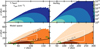 |
Fig. 1 Number density (top panels) and region of the disk included in the parameter study (bottom panels) for a typical T Tauri (L= 0.3 L⊙; left panels) and Herbig (L = 20 L⊙; right panels) disk model (see Appendix A for details). The part of the disk that is included in the physical models is shown in dark orange and is bound by the highest temperature included (40 K) and the restriction that the UV is fully shielded. Light orange denotes the region with temperatures and densities probed by our models but with some low level of UV. White contours show the regions contributing to 25% and 75% of the emission from the C18O 3–2 line. The green crosses numbered #1, #2, #3 and #4 are approximate locations of the representative models of Sect. 3.1.3. |
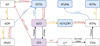 |
Fig. 2 Chemical reaction network showing the major CO destruction pathways and important competing reactions. Red arrows show reactions that are mediated directly or indirectly by cosmic-ray photons, yellow arrows show hydrogenation reactions and blue arrows show grain-surface reactions. The initial major carbon carrier (CO) is shown in grey-purple. Stable products of CO processing are denoted with blue boxes. sX denotes that species X is on the grain surface. |
Symbol overview for the rate equations.
Chemical trends with variations in parameters.
Rate coefficients for collisions with He+.
3 Results
We have performed a parameter space study of the chemistry of CO under shielded conditions in protoplanetary disks. In this section we first present the results for the physical parameters studied, namely chemical evolution time, density, temperature and cosmic-ray ionisation rate. Figure 3 focuses on the effects of time and cosmic-ray ionisation rate, while Fig. 4 focuses on the effects of temperature and density. Together these figures show that the evolution of the CO abundance depends strongly on the physical conditions assumed in the chemical model, especially the temperature, in addition to the cosmic-ray ionisation rate identified earlier. Finally, the effects of the assumed chemical parameters on four positions in physical parameter space are studied.
3.1 Physical parameter space
3.1.1 Importance of the cosmic-ray ionisation rate
Consistent with previous studies, the cosmic-ray ionisation rate is found to be the driving force behind most of the changes in the CO abundance. A higher cosmic-ray ionisation rate allows the chemistry to evolve faster, but in a similar way. As such the cosmic-ray ionisation rate and chemical evolution time are mostly degenerate. Figure 3 presents an overview of the dependence of the total CO abundance (gas plus ice) on evolution time and  . CO can be efficiently destroyed in 1–3 Myr for
  s−1 and temperatures lower than 25 K.
For models at 15 K and low densities of 106 cm−3, the CO abundance behaviour does not show the degeneracy between  and time. This is caused by the formation of NO in the ice. The NO abundance depends non-linearly on the cosmic-ray ionisation rate. A high abundance of NO in the ice lowers the abundance of available atomic H on the ice as it efficiently catalyses the formation of H2 on the ice. This effect has also been seen in Penteado et al. (2017) using the same network but under different conditions. A similar catalytic effect for the formation of H2 was first noted in the work by Tielens & Hagen (1982).
At high density and temperature (35 K, 1010 cm−3), a sequence of CO destruction and then reformation is visible in the CO abundance. The first cycle of this was also seen and discussed in Eistrup et al. (2016) and can be attributed to the lower formation rate of OH due to a decrease in the H2O abundance on Myr timescales. Some models, especially those with a cosmic-ray ionisation rate of 10−16 s−1, can have five or more of these CO–CO2 abundance inversions, while the H2O abundance continues to decrease. For the rest of the results in this section, a cosmic-ray ionisation rate of 10−17 s−1, is taken, thought to be typical for dense molecular clouds (e.g., Dalgarno 2006).
3.1.2 Importance of temperature
Figure 4 presents the total CO abundance over the entire density-temperature grid at four time steps during the evolution of the chemistry. These figures demonstrate clearly that CO is efficiently destroyed only at low temperatures, < 30 K. At early times, CO is most effectively destroyed at high densities and temperatures between 20 and 30 K. In this range, the grain-surface formation ofCO2 from the reaction between CO and OH is efficient. At these temperatures, CO is primarily in the gas phase but a small fraction resides on the grain surface where it is highly mobile. OH is created during the destruction of H2O ice. This reaction is most efficient under high-density conditions because atomic H competes with CO for reaction with the OH radical on the grain. At low densities, the relative abundance of H is higher in the models, thus greatly suppressing the formation rate of CO2 from CO + OH on the grain.
At 3 Myr CO destruction below 20 K becomes visible. The total CO abundance in this temperature range is only weakly dependent on the density: CO destruction is efficient below 16 K at the lowest densities, while it is efficient up to 19 K at the highest densities. This range is strongly correlated with the fraction of CO residing in the ice.
At late times, >5 Myr, there is a strong additional CO destruction at densities <109 cm−3 and at temperatures between 20 and 25 K.At this point, the C+ formed from the CO + He+ reaction can efficiently be converted into CH4, which freezes out on the grains.
3.1.3 Representative models
Four points in the physical parameter space have been chosen for further examination. They are chosen such that they span the range of parameters that can lead to low total CO abundances within 10 Myr and such that they sample different CO destruction routes. These points are given in Table 5 and are marked in Fig. 4. Figure 5 presents the total abundance (gas and ice) of CO and its stable reaction products as a function of time for the four physical conditions that have been chosen.
Models #1 (13 K, 108 cm−3) and #2 (18 K, 3 × 1011 cm−3) show very similar behaviours, even though they have very different densities. This is due to the combination of the active destruction pathway, CO hydrogenation, and the H2 formation prescription, which forces a constant atomic hydrogen concentration, leading to a constant CO destruction rate as a function of density. In both models, 90% of the CO has been converted into CH3OH in 2 Myr. Before this time the H2CO abundance is constant, balanced between the formation due to CO hydrogenation and destruction due to hydrogenation. As the CO abundance drops, and thus the formation rate of H2CO falls, so does its abundance. After slightly more than 2 Myr, methanol has reached a peak abundance close to 10−4. This marks the end of hydrogenation-driven chemical evolution as most molecules on the ice cannot be hydrogenated further. After this, cosmic-ray-induced dissociation dominates the abundance evolution, slowly destroying CH3OH, forming CH4 and H2O and destroying CO2 forming CO and O, both of which quickly hydrogenate to CH3OH and H2O. A small amount of CH4 is further converted into C2H6, which happens more efficiently at higher densities, due to the lower availability of atomic H.
The abundance traces for model #3 (25 K, 5 × 1011 cm−3) show two different destruction pathways for CO at a temperature where most of the CO is in the gas phase. The rise in CO2 abundance indicates that a significant portion of the CO reacts with OH on the grain-surface to form CO2. At 2 Myr, nearly 99% of the initial CO has been destroyed. Most of the CO has been incorporated into CO2 with a significant amount of carbon locked into CH4. CH4 is formed from a sequence of reactions that begin with the destruction of CO by He+. At these late times, C2H6 acts as a carbon sink, slowly locking up carbon that is created in the form of the CH3 radical from the dissociation of CH4.
The abundance traces for model #4 (21 K, 3 × 106 cm−3) are an outlier in this comparison. Most of the CO is in the gas phase at this temperature and density. It takes at least 2 Myr to destroy 50% of the CO and 5 Myr to destroy 90% of the CO. For the conditions shown here, most of the CO is destroyed in the gas phase by dissociative electron transfer with He+. This leads to the formation of hydrocarbons in the gas phase, primarily CH3 and C2H2, which freeze-out and are hydrogenated on the grain to form CH4 and C2H6 (as also seen by Aikawa et al. 1999).
Physical parameters for the chemical parameters test.
3.2 Chemical parameter space
For the four different cases listed in Table 5, a set of models with varying atunnel and fdiff have been computed. atunnel primarily changes the reaction probability for grain-surface reactions involving atomic or molecular hydrogen that have a barrier, such as sCO + sH and sOH + sH2. The value offdiff changes the speed at which species can move over the grain-surface. Models #1 and #2 are both in the region of parameter space where CO is frozen out and thus sample pure grain-surface chemistry at low temperature and density, and at a slightly higher temperature and high density, respectively. Model #3 is near the local minimum in gaseous CO abundance seen in Fig 4. Model #4 is located in a region of parameter space where most changes are still ongoing at later times. Together these four cases should sample the different dominant CO destruction pathways.
The first row of Fig. 6 shows the total CO abundance as function of chemical parameters for different times for point #1in our physical parameter space with CO mostly in the ice. There is a strong dependence on the tunnelling barrier width (atunnel). This is because the CO destruction in this temperature regime is dominated by the formation of sHCO. The sCO + sH reaction has a barrier which strongly limits this reaction, H tunnelling through this barrier thus increases the rate of CO destruction. Our fiducial value for the barrier width, 1 Å, is in the transition between slow hydrogenation at higher barrier widths and runaway hydrogenation at lower barrier widths. As such a 10% change to the barrier width around 1 Å changes the abundance of CO by a factor of ~ 3.
There are only very weak dependencies on the diffusion-to-binding energy ratio (fdiff = Ediff∕Ebind) for these very low temperatures. This points at a CO destruction process that is entirely restricted by the tunnelling efficiency of H. If the sCO + sH reaction is quenched by a large barrier, CO destruction is so slow that, due to the destruction of CO2 by cosmic-ray-induced photons, theCO abundance is actually increased from the initial value. This happens at barrier widths larger than 1.5 Å. At the lowest fdiff, CO is turned into CO2 through sCO + sOH at early times. At later times, the CO2 is destroyed, again by cosmic-ray-induced photons and more CO is formed, leading to a slower CO abundance decrease at late times.
The second row of Fig. 6 shows the total CO abundance as a function of chemical parameters for different times for point #2. Since CO is frozen out for both case #1 (T = 13 K) and #2 (T = 18 K), there are strong similarities between the first and second row of models in Fig. 6. The only significant difference can be seen at atunnel > 1.0 Å and fdiff < 0.2. With these chemical parameters and these high densities (3 × 1011 cm−3), sCO + sOHcan be an effective destruction pathway.
The third row of Fig. 6 shows the total CO abundance for point #3 in our physical parameter space at T = 25 K and n =5 × 1011 cm−3. The large and irregular variation in CO abundance in this figure points at a number of competing processes. The two main processes destroying CO at this temperature and density are again sCO + sH and sCO + sOH. These grain-surface reactions dominate the CO destruction even though CO is primarily in the gas phase. The fraction of time that CO spends on the grain is long enough to allow the aforementioned reactions to be efficient. At the smallest barrier widths (<0.7 Å), the conversion of CO into CH3OH through hydrogenation dominates the CO abundance evolution, but this pathway quickly gets inefficient if the tunnelling barrier is made wider. In the rest of the parameter space, the formation of CO2 dominates the abundance evolution.
Although CO is destroyed significantly in this model from 2 Myr onward, there is a clear region in parameter space where the CO destruction is slower. This region at high fdiff and intermediate atunnel has up to two orders of magnitude higher CO abundance compared with the rest of parameter space. The high fdiff significantly slows down all reactions that are unaffected by tunnelling. In this region of parameter space, CO mobility is significantly lower than H mobility due to the latter being able to tunnel. This suppresses the sCO + sOH route. On the other hand, the barrier is still too wide to allow efficient hydrogenation of CO. With both main destruction routes suppressed in this region, it takes longer to reach a significant amount of CO destruction. Further increasing atunnel from this point slows down the tunnelling of H and thus the formation rate of H2O. This leads into a larger OH abundance on the ice, and thus a larger CO2 formation rate.
The fourth row of Fig. 6 shows the total CO abundance at different times for point #4 at a low density of 3 × 106 cm−3 and T = 21 K. At early times there is no strong destruction of CO, after 3 Myr there is only a small region where the abundance has dropped by a factor of three. CH3OH and CO2 are formed in this region of parameter space. At 5 Myr, there is a region at low barrier width, around 0.6 Å and fdiff > 0.3, where the hydrogenation of CO has led to a large decrease in the CO abundance. At 7 Myr this process has caused a decrease of CO abundance of at least two orders of magnitude in this region. At the same time, the CO abundance over almost all of the parameter space has dropped by an order of magnitude. This is the effect of the gas phase route starting with dissociative electron transfer of CO to He+: CO + He+ → C+ + O + He. In the last 3 Myr of chemical evolution, this reaction pathway removes 99.9% of the CO in a large part of the parameter space. Only regions that had a significant build up of CO2 at early times, or where N2 can be efficiently reformed, show CO abundances >10−6, because CO is reformed from CO2 and because N2 competes with CO for reactions with He+, respectively.
In summary, our results do not strongly depend on the value of fdiff; however, the speed of hydrogenation critically depends on the value for atunnel, especially around atunnel = 1 Å. Several independent laboratory experiments show that the CO hydrogenation proceeds fast, even at temperatures as low as 10–12 K(Hiraoka et al. 2002; Watanabe & Kouchi 2002; Fuchs et al. 2009) so a high barrier is unlikely. Reaction probabilitiesfrom the Harmonic Quantum Transition State calculations by Andersson et al. (2011) are consistent with atunnel ≈ 0.9 Å in our calculations. Given the importance of the exact value of the tunnelling barrier on the chemical evolution, more work is needed in understanding the tunnelling of hydrogen during hydrogenation processes.
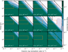 |
Fig. 3 Total CO abundance (gas and ice) as function of time and cosmic-ray ionisation rate for the fiducial chemical model. Each sub-figure has a different combination of temperature and density as denoted in the bottom left of each panel. Time and cosmic-ray ionisation rate are degenerate in most of the parameter space. The orange box denotes the combinations of |

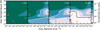 |
Fig. 4 Time evolution of CO abundance as function of gas temperature and density. Chemical evolution time is denoted in the upper right corner of each panel and ζ = 10−17 s−1 for all of these models. The orange numbers show the locations of the physical conditions taken in Sect. 3.2. |
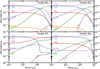 |
Fig. 5 Abundance traces of CO and its destruction products for the four points denoted in Fig. 4 with conditions as tabulated in Table 5. Plotted abundances are the sum of the gas and ice abundance for each species. |
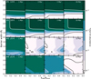 |
Fig. 6 Time evolution of total CO abundance (ice and gas) as function of the assumed tunnelling barrier width (atunnel) and diffusion-to-binding energy ratio (fdiff). All these models have |

4 Discussion
Our results show that it is possible to chemically process CO under conditions (T < 30 K, n = 106−1012 cm−3) that are representative of a large mass fraction of a protoplanetary disk on a few Myr timescale. As such, chemical processing of CO, specifically the formation of CH3OH and CO2 and on longer timescales hydrocarbons, has a significant effect on the observed CO abundance.
Our results agree with Reboussin et al. (2015), Eistrup et al. (2016) and Schwarz et al. (2018) that a significant cosmic-ray ionisation rate, > 5 × 10⁻¹⁸ s−1 in our study, is needed to convert CO.
In contrast with Furuya & Aikawa (2014) and Yu et al. (2016), we do not find that destruction of CO through reactions with He+ is a main pathway for a cosmic-ray ionisation rate of 10−17 s−1. This is mostly because this destruction timescale is >5 Myr, for these levels of ionisation. However, Furuya & Aikawa (2014) assume a higher cosmic-ray ionisation rate (5 × 10⁻¹⁷s−1) whereas Yu et al. (2016) have X-rays that add to the total ionisation rate of the gas. This lowers their CO destruction timescale significantly (Fig. 3).
4.1 When, where and how is CO destroyed within 3 Myr
There are two main reaction mechanisms that can destroy CO in 3 Myr under cold disk midplane conditions, assuming a cosmic-ray rate of 10−17 s−1: hydrogenation of CO to CH3OH and the formation of CO2. Hydrogenation of CO forming CH3OH reduces CO by an order of magnitude within 2 Myr in the cold regions of the disk where CO is completely frozen out (Fig. 5, top two panels; Fig. 7, left column, top two panels). The first step of this pathway sCO + sH has a barrier and thus the timescale of this reaction is strongly dependent on the assumed hydrogen tunnelling efficiency (atunnel), with shorter timescales at lower assumed atunnel (Fig. 6).
Contrary to Schwarz et al. (2018), we find that CH3OH formation is only dominant when CO is frozen-out, <20 K. This is probably due to the more complete grain-surface chemistry in our work, allowing other species to react with atomic H and removing it from the grain-surface before CO can react with it at higher temperatures. This leads us to conclude that CO2 formation is always the dominant CO destruction mechanism in the warm molecular layer in the first 5 Myr instead of CO hydrogenation, showing that a larger grain-surface network needs to be considered.
The second pathway, CO + OH → CO2 on the ice, is efficient at slightly higher temperatures, between the CO iceline temperature and up to 35 K at the highest densities (Fig. 4). This pathway leads to ~2 orders decrease in the CO abundance within 3 Myr. The rate of conversion of CO into CO2 depends strongly on the assumed chemical parameters in the first Myr. By 3 Myr most of these initial differences have been washed out. Only a very slow assumed diffusion rate (fbind > 0.35) leads to a CO abundance above 10−6 after 3 Myr (Fig. 6).
Production of hydrocarbons follows the formation of CH3OH in the first Myr. When the CO abundance has been lowered by 1 to 2 orders of magnitude, production of CH3OH stops, while the formation of CH4 continues. At ~3 Myr, CH4 becomes more abundant than CH3OH. At even longer timescales, CH4 gets turned into C2H6. Formation of hydrocarbons starting from CO + He+ in the gas phase is only effective at densities < 109 cm−3 between the CO and CH4 icelines. Even in this region, the timescale is >3 Myr.
The timescales for these processes scale inversely with the cosmic-ray or X-ray ionisation rate. As such, in regions with lower ionisation rates CO destruction can be slower than described here. The reverse is also true, so if locally produced energetic particles play an significant role, the CO destruction timescales become shorter.
In conclusion, for a nominal cosmic-ray ionisation rate of 10−17 s−1, CO can be significantly destroyed (orders of magnitude) in the first few Myr of disk evolution under cold conditions. This conclusion is robust against variations in chemical parameters, except if the barrier width for the CO + H tunneling becomes too large. Under warm conditions (T > 30 K), the CO abundance is lowered by a factor of a few at most.
4.2 Implications for observations
Mapping the results from the chemical models summarized above onto the physical structure seen in Fig. 1 results in Fig. 7. It is clear that CO can be destroyed over a region of the disk, that contains a significant amount of mass. For the T Tauri disk a portion of this CO destruction will be in a region of the disk where CO is not traceable by observations, as the CO is frozen out. However, there is also a significant region up to 30 K within and above the CO snow surface where CO is depleted and where the emission from the less abundant 18O and 17O isotopologues originates (Miotello et al. 2014). Thus, the processes studied here can explain, at least in part, the observations of low CO abundances within the iceline in TW Hya (Zhang et al. 2017).
If CO destruction would also be effective in disk regions that are irradiated by moderate amounts (< 1 G0) of (interstellar) UV radiation, then a region responsible for ~20% of the emission canbe depleted in CO by ~1 order of magnitude by 3 Myr, as seen in Fig. 7. The other ~ 80% is also likely affected due to mixing of CO poor gas from below the iceline into the emitting region (see Sect. 4.4). This would result in a drop of the C18O isotopologue flux between 20% and an order of magnitude depending on the vertical mixing efficiency. Rarer isotopologues, whose flux comes from lower, colder layers, would be more severely affected. The T Tauri model shown in Figs. 1 and 7 assume a total source luminosity of around 0.3 L⊙ representative of the bulk of T Tauri stars in low mass star-forming regions (Alcalá et al. 2017). For disks around stars with a lower luminosity or with higher ages, the effect of CO destruction would be even larger.
The warm upper layers exposed to modest UV have also been modelled by Schwarz et al. (2018). They find that the CO abundance is generally high in these intermediate layers, with significant CO destruction only taking place for high X-ray or cosmic ray ionisation rates. This is consistent with our Figs. 7 and A.1.
For Herbig sources, only a small region of the disk falls within the range of parameters studied here and an even smaller region is at temperatures under 30 K, while also being shielded (Fig. 1). Because Herbig disks host more luminous stars than their T Tauri counterparts, they also tend to be warmer. This means that a smaller mass fraction of the disk has temperatures between 10 and 30 K, where CO can be efficiently destroyed. As such our chemical models predict thatHerbig disk have a CO abundance that is close to canonical, consistent with observations by Kama et al. (2016).
Young disks around T Tauri stars are expected to be warmer due to the accretional heating (Harsono et al. 2015). They are also younger than the time needed to significantly convert CO to other species with grain surface reactions. As such young disks should close to canonical CO abundances, as seems to be observed for at least some disks (van ’t Hoff et al. 2018).
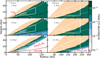 |
Fig. 7 Total CO abundance (gas and ice) from the chemical models, at 1, 3 and 10 Myr, mapped onto the temperature and density structure of a T Tauri and Herbig disk model (see Fig. A.1 and Appendix A). A cosmic-ray ionisation rate of 10−17 s−1 is assumedthroughout the disk. The orange area shows the disk region that has a temperature above 40 K and is thus not included in our chemical models. See Fig. A.1 for the CO abundance in that region using a simple CO chemistry. The white contours shows the area within which 25% and 75% of the C18O flux is emitted. The black and grey dotted lines show the 20 and 30 K contours, respectively. The Herbig disk is always warmer than 20 K. The molecules in red denote the dominant carbon carrier in the regions CO is depleted. The orange dashed line encompasses the region that is completely shielded from UV radiation (see Sect. 2.1). |
4.3 Observing chemical destruction of CO
In our models, CO is mostly processed into species that are frozen-out in most of the disk, complicating detection of these products with sub-mm lines. Several of the prominent carbon reservoirs, like CO2, CH4 and C2 H6, are symmetric molecules without a dipole moment, so they do not have detectable sub-mm lines. Even CH3OH, which does have strong microwave transitions, is difficult to detect since the processes that get methanol ice off the grains mostly destroy the molecule (e.g. Bertin et al. 2016; Walsh et al. 2016). Thus, observing the molecules in the solid state would be the best proof of this chemical processing. Another way to indirectly observe the effects chemical processing of CO would be to compare to cometary abundances. This will be discussed in Sect. 4.4.
Ice does not emit strong mid-infrared bands. However, for some highly inclined disks, the outer disk ice content can be probed with infrared absorption against the strong mid-infrared continuum of the inner disk with the line of sight passing through the intermediate height disk layers (Pontoppidan et al. 2005). The processes discussed here will leave a chemical imprint on the ice absorption spectra. The destruction pathways of CO preferentially create CO2, CH3OH, CH4 and H2O. CO2 reaches a peak abundance of ~7 × 10⁻⁵, seven times higher than the initial conditions, which would be detectable. A large CO2 ice reservoir would therefore immediately point at a conversion of CO to CO2, either in the disk or en route to the disk (Drozdovskaya et al. 2016). The formation of CH4 and CH3OH happens mostly in the coldest regions of the disk (<20 K) as such observationsof large fractions (>20% with respectto H2O) of CH4 and CH3OH in the ice would point at a disk chemistry origin of CO destruction. If large amounts of CH4 or CH3OH are found in infrared absorption spectra, this would also imply that vertical mixing plays a role in the chemical processing, as this is needed to move the CH4 and/or CH3OH ice hosting grains away from the cold midplane up to the layers that can be probed with infrared observations. For H2O the increase is generally smaller than a factor of two, so that H2O ice is not a good tracer of CO destruction.
If the gas and dust in the midplane is not static, but moves towards the star due to the accretion flow or radial drift of dust grains, then it is expected that the products of CO destruction are thermally desorbed in the inner disk (see Booth et al. 2017; Bosman et al. 2018). This would cause an observable increase in abundance. Current infrared observations of gaseous CO2 emission do not show a signal consistent with an CO2 enriched inner disk, but the optical thickness of the 15 μm CO2 lines in the surface layers might hinder the observation of CO2 near the disk midplane (Salyk et al. 2011; Pontoppidan & Blevins 2014; Walsh et al. 2015; Bosman et al. 2017, 2018). Gibb & Horne (2013) have observed gaseous CH4 in absorption in the near-infrared in GV Tau N. Their probed CH4 is rotationally hot (750 K) and is thus likely situated within the inner 1 AU of the disk. They rule out a large column of CH4 at lower temperatures (100 K). However, this disk is still embedded, so it is possibly too young to have converted CO into CH4 (Carney et al. 2016). Gaseous CH4 and CH3OH have not been detected with Spitzer-IRS in disks, but should be detectable with JWST-MIRI. If lines from these molecules are brighter than expected for inner disk chemistry, it could point at a scenario in which CO is converted to CH4 and CH3OH in the cold (<20 K) outer-midplane regions of the disk, and that the reaction products are brought into the inner disk via accretion or radial drift.
4.4 Interactions with disk dynamics
The chemical timescales needed for an order of magnitude decrease of the CO dependence are close to 2 Myr. This timescale is significantly longer than the turbulent mixing timescales, even in the outer disk. As such it is not inconceivable that either vertical mixing or gas accretion influences the abundance of CO. For both the sCO + sH and the sCO + sOH route, the rate scales with the abundance of CO in the ice: the higher the abundance, the faster the rate, although the dependence can be sub-linear. This means that, if vertical mixing replenishes the disk midplane CO reservoir, the destruction of CO can happen at a higher rate for a longer time. This converts CO to other species not only in the regions where the processes described in this paper are effective but also in the regions around it. For mixing to have a significant effect at 100 AU, a turbulent α of 10−4 or higher is needed (see, e.g., Ciesla 2010; Semenov & Wiebe 2011; Bosman et al. 2018).
The freeze-out of CO on grains that are large enough to have settled below the CO snow surface can also lower the abundance of CO in the disk atmosphere. This process is thought to happen for H2O to explain the low observed abundances of H2O in the outer disk (Hogerheijde et al. 2011; Krijt et al. 2016; Du et al. 2017). Using a toy model Kama et al. (2016) showed that the CO abundance in the disk atmosphere can be lowered by 1–2 orders of magnitude in the disk lifetime. This process can work in concert with the chemical destruction of CO to lower the CO abundance in the outer disk. If large grains are locking up a significant fraction of the CO near the midplane outside of the CO iceline, then this CO would come off the grains near the CO iceline, leading to an strong increase in the CO abundance. Zhang et al. (2017) show however that for TW Hya, this is not the case: CO also has a low abundance of ~ 3 × 10⁻⁶ within the CO iceline. Further observations will have to show if this is the case for all disks with a low CO abundance, or if TW Hya is the exception and this low CO abundance is caused by its exceptional age of ~ 8 Myr (Donaldson et al. 2016).
If the destruction of CO within the CO snowline is a general feature of protoplanetary disks, then a mechanism to stop any CO locked up in grains from being released in the gas phase will need to be considered. This is hardto do without actually halting radial drift completely, for the same reasons that it is hard to stop CO2 from desorbing off the grain at its respective snowline (Bosman et al. 2018).
The fact that comets in the solar system do contain significant amounts of CO (up to 30% with respect to H2O; Mumma & Charnley 2011; Le Roy et al. 2015) suggests that these comets were formed in a cold CO rich environment, possibly before the bulk of the CO was converted into other molecules. In other disks, such CO-rich grains must then have been trapped outside the CO iceline to prevent significant CO sublimating in the inner regions.
5 Conclusions
We performed a kinetic chemical modelling study of the destruction of CO under UV shielded, cold (<40 K) and dense (106 –1012 cm−3) conditions. Both grain-surface and gas phase routes to destroy CO are considered and their efficiencies and timescales evaluated using a gas-grain chemical network. Furthermore, we studied the effects of the assumed ice diffusion speed (through the diffusion-to-binding energy ratio, fdiff) and the assumed H and H2 tunnelling efficiency (through the tunnelling barrier width, atunnel) on the evolution of the CO abundance both in the gas phase and on the grain-surface. Our findings can be summarised as follows:
CO destruction is linearly dependent on the assumed H2 ionisation rate by energetic particles (cosmic rays, X-rays) over a large region of the considered physical parameter space. Only high enough cosmic-ray ionisation rates, >5 × 10⁻¹⁸ s−1 can destroy CO on a <3 Myr timescale (Sect. 3.1.1, Fig. 3).
The chemical processing of CO is most efficient at low temperatures. A relation between disk temperature and measured CO abundance is expected. The coldest disks would have the lowest CO abundances; in contrast, flaring disks around luminous Herbig stars should have close to canonical CO abundances.
At low temperatures, hydrogenation of CO is efficient when CO is fully frozen-out, leading to a reduction of the total CO abundance by ~2 orders assuming
 s−1. This route is only weakly dependent on the temperature and density, as long as CO is fully frozen-out (Sect. 3.1, Fig. 4).
At temperatures of 20–30 K, just above the desorption temperature of CO, formation of CO2 from the reaction of CO with OH on the ice is efficient. The CO abundance can be reduced by two orders of magnitude in 2–3 Myr for
 s−1. The formation of CO2 is more efficient at higher densities (Sect. 3.1, Fig. 4).
Gas phase destruction of CO by He+, eventually leading to the formation CH4 and H2O, only operates on timescales >5 Myr for
 s−1. Furthermore, this pathway is only effective at low densities (<109 cm−3) and in a small range of temperatures (15–25 K). As such, this pathway is not important in the context of protoplanetary disk midplanes (Sect. 3.1, Fig. 4).
The assumed tunnelling barrier width (atunnel) strongly influences the speed of CO hydrogenation with efficient tunnelling leading to fast hydrogenation of CO. The CO destruction due to CO2 formation is only weakly dependent on the assumed chemical parameters. Only when fdiff is increased above 0.35 can this reaction be slowed down (Sect. 3.2, Fig. 6).
CO2, CH3OH and, on a longer timescale, CH4 are all abundantly formed in the regions where CO is destroyed. Observations of anomalously high abundances of CH4, CH3OH or CO2 either in infrared absorption spectroscopy towards edge-on systems, or in infrared emission from the inner disk, can help in distinguishing the chemical pathway responsible for CO destruction.
Vertical mixing can bring gas from the warmer, CO richer layers to the lower colder layers, where CO can be converted into CH3OH or CO2. This would allow for the chemical processes to also lower the CO abundance in the higher, warmer layers of the disk.
In conclusion, chemical reprocessing of CO can have a significant impact on the measured disk masses if sufficient ionising radiation is present in the cold (<30 K) regions of the disk. Further modelling of individual disks will have to show to which degree chemical processes are important and where other physical processes will need to be invoked.
Acknowledgements
Astrochemistry in Leiden is supported by the European Union A-ERC grant 291141 CHEMPLAN, by the Netherlands Research School for Astronomy (NOVA), by a Royal Netherlands Academy of Arts and Sciences (KNAW) professor prize. C.W. acknowledges the University of Leeds for financial support.
Appendix A Dali protoplanetary disk models
For Fig. 1 two DALI models (Bruderer et al. 2012; Bruderer 2013) have been run to generate maps of the temperatureand radiation field for the disks given the gas and dust density structures and stellar spectra as inputs. The input parameters can be found in Table A.1. In the following, the modelling procedure is shortly reiterated.
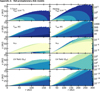 |
Fig. A.1 Gas number density, gas temperature, gas phase CO fractional abundance and UV radiation field for the T Tauri and Herbig models. A full gas-grain model was not considered for the CO abundance. Freeze-out, desorption, gas phase reactions and photodissociation are included in the chemical computation. CO abundance after 1 Myr of chemical evolution is shown. |
Adopted model parameters for T Tauri and Herbig disks.
Radially the gas and dust are distributed using a tapered power law,
![Mathematical equation: \begin{equation*} {\mathrm\Sigma}_{\mathrm{gas}} = \Sigma_c \left(\frac{R}{R_c})\right)^{-\gamma} \exp\left[-\left(\frac{R}{R_c}\right)^{2-\gamma}\right], \end{equation*}](/articles/aa/full_html/2018/10/aa33497-18/aa33497-18-eq15.png) (A.1)
(A.1)
![Mathematical equation: \begin{equation*} {\mathrm\Sigma}_{\mathrm{dust}} = \frac{{\mathrm\Sigma}_c}{{g/d}} \left(\frac{R}{R_c})\right)^{-\gamma} \exp\left[-\left(\frac{R}{R_c}\right)^{2-\gamma}\right]. \end{equation*}](/articles/aa/full_html/2018/10/aa33497-18/aa33497-18-eq16.png) (A.2)
(A.2)
Vertically the gas and dust are distributed according to a Gaussian, the dust is divided into a “large” grain and a “small” grain population (see Table A.1), the large grain population contains a fraction flarge of the mass.
![Mathematical equation: \begin{equation*} \rho_{\mathrm{gas}}(R,{\mathrm\Theta}) = \frac{{\mathrm\Sigma}_{\mathrm{gas}}(R)}{\sqrt{2\pi}Rh_{\mathrm{gas}}(R)}\exp\left[-\frac12\left(\frac{\pi/2 - {\mathrm\Theta}}{h(R)}\right)^2\right], \end{equation*}](/articles/aa/full_html/2018/10/aa33497-18/aa33497-18-eq17.png) (A.3)
(A.3)
![Mathematical equation: \begin{equation*} \rho_{\mathrm{dust,\ small}}(R,{\mathrm\Theta}) = \frac{\left(1-f_{\mathrm{large}}\right){\mathrm\Sigma}_{\mathrm{dust}}(R)}{\sqrt{2\pi}Rh_{\mathrm{gas}}(R)}\exp\left[-\frac12\left(\frac{\pi/2 - {\mathrm\Theta}}{h_{\mathrm{gas}}(R)}\right)^2\right], \end{equation*}](/articles/aa/full_html/2018/10/aa33497-18/aa33497-18-eq18.png) (A.4)
(A.4)
![Mathematical equation: \begin{equation*} \rho_{\mathrm{dust,\ large}}(R,{\mathrm\Theta}) = \frac{f_{\mathrm{large}}{\mathrm\Sigma}_{\mathrm{gas}}(R)}{\sqrt{2\pi}Rh_{\mathrm{large}}(R)}\exp\left[-\frac12\left(\frac{\pi/2 - {\mathrm\Theta}}{h_{\mathrm{large}}(R)}\right)^2\right], \end{equation*}](/articles/aa/full_html/2018/10/aa33497-18/aa33497-18-eq19.png) (A.5)
(A.5)
where  and hlarge(R) = χhgas(R). The smaller scale height for the larger grains mimics a degree of settling. The dust temperature and the radiation field are calculated using the continuum ray-tracing module of DALI. Figure A.1 shows the density, dust temperature, radiation field and fractional abundance of CO for the DALI models. The CO abundance map does not include the effects of the grain surface chemistry discussed in this paper.
Appendix B Chemical model
The abundance evolution is computed by a chemical solver based on its counterpart in the DALI code (Bruderer et al. 2012; Bruderer 2013). To solve the set of differential equations, CVODE from the SUNDAILS suite is used (Hindmarsh et al. 2005). CVODE was chosen over LIMEX, the which normally used in DALI, as CVODE is faster and more stable on the very stiff grain-surface chemistry models as well as being thread safe, enabling the calculation of multiple chemical models in parallel with OpenMP5.
B.1 Initial abundances
Table B.1 shows the input volatile abundances used in our chemical model. These abundances are depleted in Si and S but not in Fe with respect to solar. Fe will be frozen-out and will not play an active part in the chemistry.
Initial gas phase abundances for the chemical network.
Table B.2 enumerates all the binding energies used in the model. The list is sorted (left to right, top to bottom) according to molecular mass. Binding energies come from the recommended values from Penteado et al. (2017) For NH, NH2, CH, CH2 and CH3, the binding energy was increased compared with the values from Penteado et al. (2017). NH and NH2 were calculated using the method of Garrod & Herbst (2006), while for CH, CH2 and CH3 the binding energy are calculated by linearly scaling between the values for C and CH4 to the number of hydrogen atoms.
B.2 H2 formation rate
The formation of H2 is implemented following Cazaux & Tielens (2004), who give the H2 formation rate as (in H2 molecules per unit volume per unit time):
 (B.1)
(B.1)
where nH is the number density of gaseous H, vH is the thermal velocity of atomic hydrogen, Ngrain is the absolute number density of grains, agrain is the grain radius. SH(T) is the sticking efficiency (Cuppen et al. 2010), given by
 (B.2)
(B.2)
Furthermore,  is the H2 recombination efficiency given by
![Mathematical equation: \begin{equation*} \begin{split} \epsilon_{{\textrm{H}_2}} = \left(1 + \frac{1}{4} \left(1 + \sqrt{\frac{E_{\mathrm{H}_C} - E_S}{E_{\mathrm{H}_P} - E_S}}\right)^2 \exp\left[-\frac{E_S}{kT_{\mathrm{dust}}}\right] \right)^{-1} \\ \times \left[1 + \frac{v_{\mathrm{H}_C}}{2F}\exp\left(-\frac{1.5E_{\mathrm{H}_C}}{kT_{\mathrm{dust}}}\right)\left(1 + \sqrt{\frac{E_{\mathrm{H}_C} - E_S}{E_{\mathrm{H}_P} - E_S}}\right)^2\right]^{-1}, \end{split} \end{equation*}](/articles/aa/full_html/2018/10/aa33497-18/aa33497-18-eq24.png) (B.3)
(B.3)
where  K,
K,  K and ES = 200 K are the energies of a physisorbed H (HP), chemisorbedH (HC) and the energy of the saddle point between the previous two, respectively. F = 10−10 monolayers s−1 is the accretion flux of H on the ice for the H2 formation.
Binding energies for all the species in the chemical network.
B.3 Calculation of grain-surface rates
To calculate the reaction rate coefficients of grain-surface reactions, the mobility of the molecules over the grain-surface needs to be known. This requires knowledge of the vibrational frequency of a molecule in its potential well on the grain-surface (assuming a harmonic oscillator. This is the frequency at which the molecule will attempt displacements:
 (B.4)
(B.4)
where Nsites is the number of adsorption sites per grain, EX, bind is the binding energy of the molecule to the grain, agrain = 10−5 cm is the grain radius and mX is the mass of the molecule. The hopping rate is the vibrational frequency multiplied by the hopping probability, which in the thermal case is:
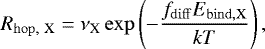 (B.5)
(B.5)
where k is the Boltzmann constant and T is the dust-grain temperature. For atomic and molecular hydrogen, tunnelling is also allowed:
![Mathematical equation: \begin{equation*} R_{\mathrm{hop,\ tunnel,\ X}} = \nu_{\textrm{X}} \exp\left[-\frac{2 a_{\mathrm{tunnel}}}{\hbar}\sqrt{2\mu f_{\mathrm{diff}} E_{\mathrm{bind, X}}}\right]. \end{equation*}](/articles/aa/full_html/2018/10/aa33497-18/aa33497-18-eq29.png) (B.6)
(B.6)
For atomic and molecular hydrogen, the fastest of these two rates is used which will almost always be the thermal rate. Only for models with a high fdiff, low atunnel and low temperature is tunnelling faster than thermal hopping.
The rate coefficient for a grain-surface reaction between species X and Y forming product(s) Z on the grain-surface is given by
![Mathematical equation: \begin{equation*} \begin{split}k({\textrm{X} + \textrm{Y}}, \textrm{Z}) = \min\left[ 1, \left(\frac{N^2_{\mathrm{act}} N^2_{\mathrm{sites}} n_{\mathrm{grain}}}{n^2_{\mathrm{ice}}}\right)\right] P_{\mathrm{reac}}({\textrm{X} + \textrm{Y}}, \textrm{Z}) \\ \left( \frac{R_{\mathrm{hop,\ X}}}{N_{\mathrm{sites}}} + \frac{R_{\mathrm{hop,\ Y}}}{N_{\mathrm{sites}}} \right) \\ = C_{\mathrm{grain}} P_{\mathrm{reac}}({\textrm{X} + \textrm{Y}}, \textrm{Z}) \left(R_{\mathrm{hop,\ X}} + R_{\mathrm{hop,\ Y}} \right) \end{split} \end{equation*}](/articles/aa/full_html/2018/10/aa33497-18/aa33497-18-eq30.png) (B.7)
(B.7)
where Nact = 2 is the number of chemically active layers, Nsites = 106 is the number of molecules per ice monolayer, ngrain = 2.2 × 10⁻¹²ngas is the number density of grains with respect to H2 and nice is the total number density of species on the grain. Preac(X + Y, Z) is the reaction probability for the reaction. This includes the branching ratios if multiple products are possible as well as a correction for reactions that have a barrier.
The reaction probability is given by
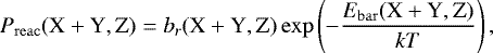 (B.8)
(B.8)
where br(X + Y, Z) is the branching ratio, Ebar(X + Y, Z) is the energy barrier for the reaction.If either H or H2 is participating in the reaction, tunnelling is included:
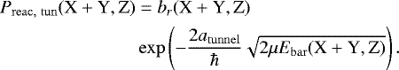 (B.9)
(B.9)
The largest of the tunnelling and thermal crossing probability is taken for the actual rate calculation, for most reactions tunnelling dominates in contrast with hopping, where thermal crossing dominates.
B.4 Implications of modelling assumptions
B.4.1 Variations in the H2 formation rate
The formation speed of H2 from atomic hydrogen is very important in our models as, together with the destruction rate of H2, it sets the abundance of atomic hydrogen in the gas. For the formation rate, the prescription of Cazaux & Tielens (2004) is used. The formalism forces the atomic H gaseous abundance to ~ 1 cm−3 for  s−1 irrespective of total gas density. A higher or lower atomic hydrogen abundance would strongly affect both the sCO + sH route, which would increase in effectiveness with higher atomic hydrogen abundances, and the sCO + sOH route, which would decrease in effectiveness with higher atomic hydrogen abundances.
B.4.2 Initial conditions
The initial conditions for the chemistry are shown in Table. B.1. The focus was on testing the CO destruction, hence we start with CO as the major volatile carbon reservoir, with trace amounts of CO2 (10% of CO) and CH3OH (1% of CO). At the densities considered here, there is no strong chemical alteration before freeze-out and desorption are balanced. Furthermore, a small portion of N is in NH3, with the rest of the nitrogen in N2.
The initial conditions can have a significant impact on the evolution of the CO abundances. The amount of H2O ice on the grains determines the formation rate of OH on the grain, which in turn impacts the transformation of CO to CO2. If the chemical evolution is started with a larger portion of carbon in hydrocarbons than assumed in this work, with the excess oxygen put into H2O, then a shorter CO destruction timescale will be found in the regions where CO2 formation is effective.
The timescale of the CO + He+ route is especially sensitive to the initial abundances. Starting with a significant fraction of the CO already incorporated into CO2, such as predicted by Drozdovskaya et al. (2016) and as observed in ices in collapsing envelopes (Pontoppidan et al. 2008), can shorten chemical timescales significantly. Chemical timescales can be further shortened by the removal of N2 from the gas phase, such as by starting the chemical model with NH3 as the dominant nitrogen carrier.
The timescale of the sCO + sH route is not very sensitive to the initial abundances, as long as they are molecular. The maximal amount of CO removal is a function of the amount of CO2 in the ice initially, but as hydrogenation of CO is at least two orders of magnitude faster than the dissociation of CO2 due to cosmic rays, this means that even when CO2 is the dominant carbon reservoir, the CO abundance can still be reduced below 10−6 by sCO + sH even with the CO replenishment.
B.4.3 Chemically active surface
All our models assume that only the molecules in the top two layers of our ices are participating in chemical reactions. The composition of these layers is assumed to be the same of that of the bulk ice. If the number of layers that can participate in chemical reactions is doubled, then the timescales for all grain-surface reactions decrease by a factor of four (see Eq. (B.7)). However, most of our grain-surface reactions are not limited by the speed of the grain-surface reactions, but by the availability of H-atoms and OH-radicals in the ice. The availability of H-atoms is set by the arrival rate of H-atoms on the grains, and this linearly depends on the total grain-surface but not on the number of chemically active layers. The availability of the OH radical is primarily set by the destruction rate of H2O which is independent of the ice thickness. As such the effect of changing the number of active layers is mostly in setting the exact location of the icelines as a larger number of active layers results in a faster sublimation rate at equal temperatures. Varying the number of active layers between one and eight changes the iceline temperature by less than 1.5 K. This effect is similar to the effect of an one order of magnitude change in the total density.
The total amount of grain-surface, and thus the assummed size of the grains does have some effect on the timescales of CO destruction. The atomic hydrogen arrival rate on the grain scales with the total available surface, which decreases if the grain size is increased and the gas-to-dust mass ratio is held fixed. However, the H2 formation rate as calculated by Cazaux & Tielens (2004) also depends on the total surface area, thus if the total surface area is decreased, that means that the abundance of atomic hydrogen should increase, cancelling the effect of the grain size on the hydrogenation reaction of CO. The production of CO2 actually increases with increasing grain size (and thus decreasing surface area). As the total grain-surface area decreases, a smaller amount of the cosmic-ray-induced UV photons are absorbed by the dust grains, as such the dissociation rate for H2O should be slightly higher, creating more OH radicals and thus increasing the rate of CO2 production.
B.4.4 Mixed ice model
The code assumes a perfectly mixed ice, that is to say that all species are assumed to be present in the upper chemically active layers at the relative abundances that they are included in the bulk of the ice. Observations of dark clouds indicate that in that stage ice mantles are not perfectly mixed, but have a layered structure (Tielens et al. 1991; Boogert et al. 2015) with a CO-rich layer on top of the H2 O-rich layers. It is expected that ice mantles in protoplanetary disks are also layered. The perfect mixing assumption can have some profound effects on the chemistry of CO. A layered ice below the CO freeze-out temperature would have a higher fraction of CO in the surface layers than currently assumed. This would initially speed-up the formation of CH3OH, however, as the CO in the top layers is converted into CH3OH, the rate of CO destruction would go down. At that point, the CO destruction rate would be dependent on the CO exchange rate of the bulk ice and the surface layers which is expected to be slower than the surface diffusion speed. Just above the CO freeze-out temperature, the top layers of the ice would be made up of mostly CH3OH, CO2 and CH4. Since the top layers have very little H2O, this would lead to very low abundances of OH radicals in the surface layers and might thus quench the sCO + sOH route to form CO2.
Mixing of an ice through bulk diffusion is a slow process. However, in the high density midplanes another process can mix ices: grain-grain collisions. In large parts of the disk, the grain size distribution is in coagulation–fragmentation equilibrium. Especially the destructive collisions leading to cratering and fragmentation should be able to mix up the layered structure.
Multi-phase models that include layering explicitly have been developed (e.g. Taquet et al. 2012; Furuya et al. 2016). Drozdovskaya et al. (2016) compared the results from their two-phase (gas and ice) chemical model to the three-phase (gas, surface ice and bulk ice) chemical model from Furuya et al. (2015). They conclude that the two-phase model and the three-phase model that includes swapping between bulk and surface ice produces comparable amounts of CO2 in the ice, but that if swapping is excluded, CO2 production is efficiently quenched. More detailed models of disk midplanes that included layering should be done in the future to better quantify the effects of assuming a fully mixed ice on the results presented here.
B.4.5 CO binding energy
The bindingenergy of CO depends strongly on the surface on which it is frozen (Collings et al. 2003; Acharyya et al. 2007). Here the binding energy of CO on a pure CO ice surface is used, which is applicable to the cold (< 20 K) regions, where CO is primarily in the ice. In warmer regions however, CO will mostly be bound to CO2, CH3OH and H2O, slightly increasing the binding energy of CO (Collings et al. 2003; Acharyya et al. 2007; Noble et al. 2012). The higher binding energy, and thus slower CO diffusion, moves upwards and broadens the temperature range over which the reaction to form CO2 (Eq. (3)) is efficient.
References
- Acharyya, K., Fuchs, G. W., Fraser, H. J., van Dishoeck, E. F., & Linnartz, H. 2007, A&A, 466, 1005 [NASA ADS] [CrossRef] [EDP Sciences] [Google Scholar]
- Aikawa, Y., Umebayashi, T., Nakano, T., & Miyama, S. M. 1999, ApJ, 519, 705 [NASA ADS] [CrossRef] [Google Scholar]
- Alcalá, J. M., Manara, C. F., Natta, A., et al. 2017, A&A, 600, A20 [NASA ADS] [CrossRef] [EDP Sciences] [Google Scholar]
- Andersson, S., Goumans, T. P. M., & Arnaldsson, A. 2011, Chem. Phys. Lett., 513, 31 [NASA ADS] [CrossRef] [Google Scholar]
- Ansdell, M., Williams, J. P., van der Marel, N., et al. 2016, ApJ, 828, 46 [Google Scholar]
- Arasa, C., van Hemert, M. C., van Dishoeck, E. F., & Kroes, G. J. 2013, J. Phys. Chem. A, 117, 7064 [CrossRef] [Google Scholar]
- Baruteau, C., Crida, A., Paardekooper, S.-J., et al. 2014, Protostars and Planets VI, 667 [Google Scholar]
- Bergin, E. A., Cleeves, L. I., Gorti, U., et al. 2013, Nature, 493, 644 [NASA ADS] [CrossRef] [PubMed] [Google Scholar]
- Bergin, E. A., & Williams, J. P. 2017, in Astrophysics and Space Science Library, eds. M. Pessah & O. Gressel, 445, 1 [Google Scholar]
- Bertin, M., Romanzin, C., Doronin, M., et al. 2016, ApJ, 817, L12 [NASA ADS] [CrossRef] [Google Scholar]
- Birnstiel, T., Dullemond, C. P., & Brauer, F. 2010, A&A, 513, A79 [NASA ADS] [CrossRef] [EDP Sciences] [Google Scholar]
- Bolatto, A. D., Wolfire, M., & Leroy, A. K. 2013, ARA&A, 51, 207 [Google Scholar]
- Boogert, A. C. A., Gerakines, P. A., & Whittet, D. C. B. 2015, ARA&A, 53, 541 [Google Scholar]
- Booth, R. A., Clarke, C. J., Madhusudhan, N., & Ilee, J. D. 2017, MNRAS, 469, 3994 [NASA ADS] [CrossRef] [Google Scholar]
- Bosman, A. D., Bruderer, S., & van Dishoeck E. F. 2017, A&A, 601, A36 [NASA ADS] [CrossRef] [EDP Sciences] [Google Scholar]
- Bosman, A. D., Tielens, A. G. G. M., & van Dishoeck E. F. 2018, A&A, 611, A80 [NASA ADS] [CrossRef] [EDP Sciences] [Google Scholar]
- Brauer, F., Dullemond, C. P., & Henning, T. 2008, A&A, 480, 859 [NASA ADS] [CrossRef] [EDP Sciences] [Google Scholar]
- Brown, W. A., & Bolina, A. S. 2007, MNRAS, 374, 1006 [NASA ADS] [CrossRef] [Google Scholar]
- Bruderer, S. 2013, A&A, 559, A46 [NASA ADS] [CrossRef] [EDP Sciences] [Google Scholar]
- Bruderer, S., Doty, S. D., & Benz, A. O. 2009, ApJS, 183, 179 [NASA ADS] [CrossRef] [Google Scholar]
- Bruderer, S., van Dishoeck, E. F., Doty, S. D., & Herczeg, G. J. 2012, A&A, 541, A91 [NASA ADS] [CrossRef] [EDP Sciences] [Google Scholar]
- Carney, M. T., Y"i"ld"i"z, U. A., Mottram, J. C., et al. 2016, A&A, 586, A44 [NASA ADS] [CrossRef] [EDP Sciences] [Google Scholar]
- Cazaux, S., & Tielens, A. G. G. M. 2004, ApJ, 604, 222 [NASA ADS] [CrossRef] [Google Scholar]
- Chen, Y.-J., Chuang, K.-J., Muñoz Caro, G. M., et al. 2014, ApJ, 781, 15 [Google Scholar]
- Ciesla, F. J. 2010, ApJ, 723, 514 [NASA ADS] [CrossRef] [Google Scholar]
- Cleeves, L. I., Bergin, E. A., Qi, C., Adams, F. C., & Öberg, K. I. 2015, ApJ, 799, 204 [NASA ADS] [CrossRef] [Google Scholar]
- Collings, M. P., Dever, J. W., Fraser, H. J., & McCoustra, M. R. S. 2003, Ap&SS, 285, 633 [NASA ADS] [CrossRef] [Google Scholar]
- Cooke, I. R., Öberg, K. I., Fayolle, E. C., Peeler, Z., & Bergner, J. B. 2018, ApJ, 852, 75 [NASA ADS] [CrossRef] [Google Scholar]
- Cuppen, H. M., & Herbst, E. 2007, ApJ, 668, 294 [Google Scholar]
- Cuppen, H. M., van Dishoeck, E. F., Herbst, E., & Tielens, A. G. G. M. 2009, A&A, 508, 275 [NASA ADS] [CrossRef] [EDP Sciences] [Google Scholar]
- Cuppen, H. M., Ioppolo, S., Romanzin, C., & Linnartz, H. 2010, Phys. Chem. Chem. Phys., 12, 12077 [NASA ADS] [CrossRef] [Google Scholar]
- Cuppen, H. M., Walsh, C., Lamberts, T., et al. 2017, Space Sci. Rev., 212, 1 [NASA ADS] [CrossRef] [Google Scholar]
- Dalgarno, A. 2006, Proc. Natl. Acad. Sci., 103, 12269 [NASA ADS] [CrossRef] [Google Scholar]
- Donaldson, J. K., Weinberger, A. J., Gagné, J., et al. 2016, ApJ, 833, 95 [NASA ADS] [CrossRef] [Google Scholar]
- Draine, B. T. 1978, ApJS, 36, 595 [NASA ADS] [CrossRef] [Google Scholar]
- Draine, B. T.,& Lee, H. M. 1984, ApJ, 285, 89 [Google Scholar]
- Drozdovskaya,M. N., Walsh, C., van Dishoeck, E. F., et al. 2016, MNRAS, 462, 977 [NASA ADS] [CrossRef] [Google Scholar]
- Du, F., Bergin, E. A., & Hogerheijde, M. R. 2015, ApJ, 807, L32 [NASA ADS] [CrossRef] [Google Scholar]
- Du, F., Bergin, E. A., Hogerheijde, M., et al. 2017, ApJ, 842, 98 [NASA ADS] [CrossRef] [Google Scholar]
- Dutrey, A., Guilloteau, S., & Guelin, M. 1997, A&A, 317, L55 [NASA ADS] [Google Scholar]
- Eistrup, C., Walsh, C., & van Dishoeck E. F. 2016, A&A, 595, A83 [NASA ADS] [CrossRef] [EDP Sciences] [Google Scholar]
- Eistrup, C., Walsh, C., & van Dishoeck E. F. 2018, A&A, 613, A14 [NASA ADS] [CrossRef] [EDP Sciences] [Google Scholar]
- Favre, C., Cleeves, L. I., Bergin, E. A., Qi, C., & Blake, G. A. 2013, ApJ, 776, L38 [NASA ADS] [CrossRef] [Google Scholar]
- Fayolle, E. C., Öberg, K. I., Cuppen, H. M., Visser, R., & Linnartz, H. 2011, A&A, 529, A74 [NASA ADS] [CrossRef] [EDP Sciences] [Google Scholar]
- Fuchs, G. W., Cuppen, H. M., Ioppolo, S., et al. 2009, A&A, 505, 629 [NASA ADS] [CrossRef] [EDP Sciences] [Google Scholar]
- Furuya, K., & Aikawa, Y. 2014, ApJ, 790, 97 [NASA ADS] [CrossRef] [Google Scholar]
- Furuya, K., Aikawa, Y., Hincelin, U., et al. 2015, A&A, 584, A124 [NASA ADS] [CrossRef] [EDP Sciences] [Google Scholar]
- Furuya, K., van Dishoeck, E. F., & Aikawa, Y. 2016, A&A, 586, A127 [NASA ADS] [CrossRef] [EDP Sciences] [Google Scholar]
- Garrod, R. T., & Herbst, E. 2006, A&A, 457, 927 [NASA ADS] [CrossRef] [EDP Sciences] [Google Scholar]
- Garrod, R. T., & Pauly, T. 2011, ApJ, 735, 15 [NASA ADS] [CrossRef] [Google Scholar]
- Garrod, R. T., Widicus Weaver, S. L., & Herbst, E. 2008, ApJ, 682, 283 [NASA ADS] [CrossRef] [Google Scholar]
- Gibb, E. L., & Horne, D. 2013, ApJ, 776, L28 [NASA ADS] [CrossRef] [Google Scholar]
- Harsono, D., Bruderer, S., & van Dishoeck E. F. 2015, A&A, 582, A41 [NASA ADS] [CrossRef] [EDP Sciences] [Google Scholar]
- Hasegawa, T. I., Herbst, E., & Leung, C. M. 1992, ApJS, 82, 167 [NASA ADS] [CrossRef] [Google Scholar]
- He, J., & Vidali, G. 2014, ApJ, 788, 50 [NASA ADS] [CrossRef] [Google Scholar]
- Hincelin, U., Chang, Q., & Herbst, E. 2015, A&A, 574, A24 [NASA ADS] [CrossRef] [EDP Sciences] [Google Scholar]
- Hindmarsh, A. C., Brown, P. N., Grant, K. E., et al. 2005, ACM Trans. Math. Softw., 31, 363 [Google Scholar]
- Hiraoka, K., Sato, T., Sato, S., et al. 2002, ApJ, 577, 265 [NASA ADS] [CrossRef] [Google Scholar]
- Hogerheijde, M. R., Bergin, E. A., Brinch, C., et al. 2011, Science, 334, 338 [NASA ADS] [CrossRef] [PubMed] [Google Scholar]
- Ioppolo, S., Fedoseev, G., Lamberts, T., Romanzin, C., & Linnartz, H. 2013, Rev. Sci. Instrum., 84, 073112 [NASA ADS] [CrossRef] [Google Scholar]
- Johansen, A., Blum, J., Tanaka, H., et al. 2014, in Protostars and Planets VI, eds. H. Beuther, R. Klessen, C. Dullemond, & T. Henning (Tucson: University of Arizona Press), 547 [Google Scholar]
- Kama, M., Bruderer, S., van Dishoeck, E. F., et al. 2016, A&A, 592, A83 [NASA ADS] [CrossRef] [EDP Sciences] [Google Scholar]
- Kley, W., & Nelson, R. P. 2012, ARA&A, 50, 211 [NASA ADS] [CrossRef] [Google Scholar]
- Krijt, S., Ciesla, F. J., & Bergin, E. A. 2016, ApJ, 833, 285 [NASA ADS] [CrossRef] [Google Scholar]
- Lamberts, T., Cuppen, H. M., Ioppolo, S., & Linnartz, H. 2013, Phys. Chem. Chem. Phys., 15, 8287 [CrossRef] [Google Scholar]
- Lauck, T., Karssemeijer, L., Shulenberger, K., et al. 2015, ApJ, 801, 118 [NASA ADS] [CrossRef] [Google Scholar]
- Le Roy, L., Altwegg, K., Balsiger, H., et al. 2015, A&A, 583, A1 [Google Scholar]
- Lee, H.-H., Herbst, E., Pineau des Forets, G., Roueff, E., & Le Bourlot, J. 1996, A&A, 311, 690 [NASA ADS] [Google Scholar]
- Long, F., Herczeg, G. J., Pascucci, I., et al. 2017, ApJ, 844, 99 [NASA ADS] [CrossRef] [Google Scholar]
- Manara, C. F., Rosotti, G., Testi, L., et al. 2016, A&A, 591, L3 [NASA ADS] [CrossRef] [EDP Sciences] [Google Scholar]
- McClure, M. K., Bergin, E. A., Cleeves, L. I., et al. 2016, ApJ, 831, 167 [NASA ADS] [CrossRef] [Google Scholar]
- McElroy, D., Walsh, C., Markwick, A. J., et al. 2013, A&A, 550, A36 [NASA ADS] [CrossRef] [EDP Sciences] [Google Scholar]
- Miotello, A., Bruderer, S., & van Dishoeck E. F. 2014, A&A, 572, A96 [NASA ADS] [CrossRef] [EDP Sciences] [Google Scholar]
- Miotello, A., van Dishoeck, E. F., Kama, M., & Bruderer, S. 2016, A&A, 594, A85 [NASA ADS] [CrossRef] [EDP Sciences] [Google Scholar]
- Miotello, A., van Dishoeck, E. F., Williams, J. P., et al. 2017, A&A, 599, A113 [NASA ADS] [CrossRef] [EDP Sciences] [Google Scholar]
- Molyarova, T., Akimkin, V., Semenov, D., et al. 2017, ApJ, 849, 130 [NASA ADS] [CrossRef] [Google Scholar]
- Muñoz Caro, G. M., Jiménez-Escobar, A., Martín-Gago, J. Á., et al. 2010, A&A, 522, A108 [NASA ADS] [CrossRef] [EDP Sciences] [Google Scholar]
- Muñoz Caro, G. M., Chen, Y.-J., Aparicio, S., et al. 2016, A&A, 589, A19 [NASA ADS] [CrossRef] [EDP Sciences] [Google Scholar]
- Mumma, M. J., & Charnley, S. B. 2011, ARA&A, 49, 471 [NASA ADS] [CrossRef] [Google Scholar]
- Noble, J. A., Congiu, E., Dulieu, F., & Fraser, H. J. 2012, MNRAS, 421, 768 [NASA ADS] [Google Scholar]
- Oba, Y., Watanabe, N., Kouchi, A., Hama, T., & Pirronello, V. 2010, ApJ, 712, L174 [NASA ADS] [CrossRef] [Google Scholar]
- Öberg, K. I., Fuchs, G. W., Awad, Z., et al. 2007, ApJ, 662, L23 [NASA ADS] [CrossRef] [Google Scholar]
- Öberg, K. I., Garrod, R. T., van Dishoeck, E. F., & Linnartz, H. 2009a, A&A, 504, 891 [NASA ADS] [CrossRef] [EDP Sciences] [Google Scholar]
- Öberg, K. I., Linnartz, H., Visser, R., & van Dishoeck E. F. 2009b, ApJ, 693, 1209 [NASA ADS] [CrossRef] [Google Scholar]
- Öberg, K. I., van Dishoeck, E. F., & Linnartz, H. 2009c, A&A, 496, 281 [NASA ADS] [CrossRef] [EDP Sciences] [Google Scholar]
- Paardekooper, D. M., Fedoseev, G., Riedo, A., & Linnartz, H. 2016, A&A, 596, A72 [NASA ADS] [CrossRef] [EDP Sciences] [Google Scholar]
- Pascucci, I., Testi, L., Herczeg, G. J., et al. 2016, ApJ, 831, 125 [NASA ADS] [CrossRef] [Google Scholar]
- Penteado, E. M., Walsh, C., & Cuppen, H. M. 2017, ApJ, 844, 71 [NASA ADS] [CrossRef] [Google Scholar]
- Pontoppidan, K. M., & Blevins, S. M. 2014, Faraday Discuss., 169, 49 [NASA ADS] [CrossRef] [Google Scholar]
- Pontoppidan, K. M., Dullemond, C. P., van Dishoeck, E. F., et al. 2005, ApJ, 622, 463 [NASA ADS] [CrossRef] [Google Scholar]
- Pontoppidan, K. M., Boogert, A. C. A., Fraser, H. J., et al. 2008, ApJ, 678, 1005 [NASA ADS] [CrossRef] [Google Scholar]
- Reboussin, L., Wakelam, V., Guilloteau, S., Hersant, F., & Dutrey, A. 2015, A&A, 579, A82 [NASA ADS] [CrossRef] [EDP Sciences] [Google Scholar]
- Salyk, C., Pontoppidan, K. M., Blake, G. A., Najita, J. R., & Carr, J. S. 2011, ApJ, 731, 130 [NASA ADS] [CrossRef] [Google Scholar]
- Schwarz, K. R., Bergin, E. A., Cleeves, L. I., et al. 2016, ApJ, 823, 91 [NASA ADS] [CrossRef] [Google Scholar]
- Schwarz, K. R., Bergin, E. A., Cleeves, L. I., et al. 2018, ApJ, 856, 85 [NASA ADS] [CrossRef] [Google Scholar]
- Semenov, D., & Wiebe, D. 2011, ApJS, 196, 25 [NASA ADS] [CrossRef] [Google Scholar]
- Senevirathne, B., Andersson, S., Dulieu, F., & Nyman, G. 2017, Mol. Astrophys., 6, 59 [NASA ADS] [CrossRef] [Google Scholar]
- Shen, C. J., Greenberg, J. M., Schutte, W. A., & van Dishoeck E. F. 2004, A&A, 415, 203 [NASA ADS] [CrossRef] [EDP Sciences] [Google Scholar]
- Taquet, V., Ceccarelli, C., & Kahane, C. 2012, A&A, 538, A42 [NASA ADS] [CrossRef] [EDP Sciences] [Google Scholar]
- Tielens, A. G. G. M., & Hagen, W. 1982, A&A, 114, 245 [Google Scholar]
- Tielens, A. G. G. M., Tokunaga, A. T., Geballe, T. R., & Baas, F. 1991, ApJ, 381, 181 [NASA ADS] [CrossRef] [PubMed] [Google Scholar]
- Trapman, L., Miotello, A., Kama, M., van Dishoeck, E. F., & Bruderer, S. 2017, A&A, 605, A69 [NASA ADS] [CrossRef] [EDP Sciences] [Google Scholar]
- van Dishoeck, E. F., & Black, J. H. 1987, in Physical Processes in Interstellar Clouds, ed. G. E. Morfill & M. Scholer, in NATO ASIC Proc., 210, 241 [Google Scholar]
- van Dishoeck, E. F., & Black, J. H. 1988, ApJ, 334, 771 [NASA ADS] [CrossRef] [Google Scholar]
- van ’t, M. L. R., Tobin, J. J., Harsono, D., & van Dishoeck E. F. 2018, A&A, 615, A83 [NASA ADS] [CrossRef] [EDP Sciences] [Google Scholar]
- van Zadelhoff, G.-J., van Dishoeck, E. F., Thi, W.-F., & Blake, G. A. 2001, A&A, 377, 566 [NASA ADS] [CrossRef] [EDP Sciences] [Google Scholar]
- van Zadelhoff, G.-J., Aikawa, Y., Hogerheijde, M. R., & van Dishoeck E. F. 2003, A&A, 397, 789 [NASA ADS] [CrossRef] [EDP Sciences] [Google Scholar]
- Viala, Y. P., Letzelter, C., Eidelsberg, M., & Rostas, F. 1988, A&A, 193, 265 [NASA ADS] [Google Scholar]
- Visser, R., van Dishoeck, E. F., & Black, J. H. 2009, A&A, 503, 323 [NASA ADS] [CrossRef] [EDP Sciences] [Google Scholar]
- Wakelam, V., Ruaud, M., Hersant, F., et al. 2016, A&A, 594, A35 [NASA ADS] [CrossRef] [EDP Sciences] [Google Scholar]
- Walsh, C., Millar, T. J., & Nomura, H. 2010, ApJ, 722, 1607 [NASA ADS] [CrossRef] [Google Scholar]
- Walsh, C., Nomura, H., Millar, T. J., & Aikawa, Y. 2012, ApJ, 747, 114 [NASA ADS] [CrossRef] [Google Scholar]
- Walsh, C., Nomura, H., & van Dishoeck E. 2015, A&A, 582, A88 [NASA ADS] [CrossRef] [EDP Sciences] [Google Scholar]
- Walsh, C., Loomis, R. A., Öberg, K. I., et al. 2016, ApJ, 823, L10 [NASA ADS] [CrossRef] [Google Scholar]
- Watanabe, N.,& Kouchi, A. 2002, ApJ, 571, L173 [NASA ADS] [CrossRef] [Google Scholar]
- Watanabe, N., Mouri, O., Nagaoka, A., et al. 2007, ApJ, 668, 1001 [NASA ADS] [CrossRef] [Google Scholar]
- Weidenschilling, S. J. 1977, MNRAS, 180, 57 [NASA ADS] [CrossRef] [Google Scholar]
- Weingartner, J. C., & Draine, B. T. 2001, ApJ, 548, 296 [NASA ADS] [CrossRef] [Google Scholar]
- Williams, J. P., & Best, W. M. J. 2014, ApJ, 788, 59 [NASA ADS] [CrossRef] [Google Scholar]
- Woon, D. E. 2002, ApJ, 569, 541 [NASA ADS] [CrossRef] [Google Scholar]
- Yu, M., Willacy, K., Dodson-Robinson, S. E., Turner, N. J., & Evans, II, N. J. 2016, ApJ, 822, 53 [NASA ADS] [CrossRef] [Google Scholar]
- Zhang, K., Bergin, E. A., Blake, G. A., Cleeves, L. I., & Schwarz, K. R. 2017, Nat. Astron., 1, 0130 [NASA ADS] [CrossRef] [Google Scholar]
Specifically, H2O is in the upper layers of the ice, but by construction our ice mantles are perfectly mixed.
All Tables
All Figures
|
Fig. 1 Number density (top panels) and region of the disk included in the parameter study (bottom panels) for a typical T Tauri (L= 0.3 L⊙; left panels) and Herbig (L = 20 L⊙; right panels) disk model (see Appendix A for details). The part of the disk that is included in the physical models is shown in dark orange and is bound by the highest temperature included (40 K) and the restriction that the UV is fully shielded. Light orange denotes the region with temperatures and densities probed by our models but with some low level of UV. White contours show the regions contributing to 25% and 75% of the emission from the C18O 3–2 line. The green crosses numbered #1, #2, #3 and #4 are approximate locations of the representative models of Sect. 3.1.3. |
| In the text | |
|
Fig. 2 Chemical reaction network showing the major CO destruction pathways and important competing reactions. Red arrows show reactions that are mediated directly or indirectly by cosmic-ray photons, yellow arrows show hydrogenation reactions and blue arrows show grain-surface reactions. The initial major carbon carrier (CO) is shown in grey-purple. Stable products of CO processing are denoted with blue boxes. sX denotes that species X is on the grain surface. |
| In the text | |
|
Fig. 3 Total CO abundance (gas and ice) as function of time and cosmic-ray ionisation rate for the fiducial chemical model. Each sub-figure has a different combination of temperature and density as denoted in the bottom left of each panel. Time and cosmic-ray ionisation rate are degenerate in most of the parameter space. The orange box denotes the combinations of |
| In the text | |
|
Fig. 4 Time evolution of CO abundance as function of gas temperature and density. Chemical evolution time is denoted in the upper right corner of each panel and ζ = 10−17 s−1 for all of these models. The orange numbers show the locations of the physical conditions taken in Sect. 3.2. |
| In the text | |
|
Fig. 5 Abundance traces of CO and its destruction products for the four points denoted in Fig. 4 with conditions as tabulated in Table 5. Plotted abundances are the sum of the gas and ice abundance for each species. |
| In the text | |
|
Fig. 6 Time evolution of total CO abundance (ice and gas) as function of the assumed tunnelling barrier width (atunnel) and diffusion-to-binding energy ratio (fdiff). All these models have |
| In the text | |
|
Fig. 7 Total CO abundance (gas and ice) from the chemical models, at 1, 3 and 10 Myr, mapped onto the temperature and density structure of a T Tauri and Herbig disk model (see Fig. A.1 and Appendix A). A cosmic-ray ionisation rate of 10−17 s−1 is assumedthroughout the disk. The orange area shows the disk region that has a temperature above 40 K and is thus not included in our chemical models. See Fig. A.1 for the CO abundance in that region using a simple CO chemistry. The white contours shows the area within which 25% and 75% of the C18O flux is emitted. The black and grey dotted lines show the 20 and 30 K contours, respectively. The Herbig disk is always warmer than 20 K. The molecules in red denote the dominant carbon carrier in the regions CO is depleted. The orange dashed line encompasses the region that is completely shielded from UV radiation (see Sect. 2.1). |
| In the text | |
|
Fig. A.1 Gas number density, gas temperature, gas phase CO fractional abundance and UV radiation field for the T Tauri and Herbig models. A full gas-grain model was not considered for the CO abundance. Freeze-out, desorption, gas phase reactions and photodissociation are included in the chemical computation. CO abundance after 1 Myr of chemical evolution is shown. |
| In the text | |
Current usage metrics show cumulative count of Article Views (full-text article views including HTML views, PDF and ePub downloads, according to the available data) and Abstracts Views on Vision4Press platform.
Data correspond to usage on the plateform after 2015. The current usage metrics is available 48-96 hours after online publication and is updated daily on week days.
Initial download of the metrics may take a while.