| Issue |
A&A
Volume 618, October 2018
|
|
|---|---|---|
| Article Number | A51 | |
| Number of page(s) | 13 | |
| Section | The Sun | |
| DOI | https://doi.org/10.1051/0004-6361/201833101 | |
| Published online | 12 October 2018 | |
A persistent quiet-Sun small-scale tornado
I. Characteristics and dynamics⋆
1
Institute for Astronomy, Astrophysics, Space Applications and Remote Sensing, National Observatory of Athens, 15236 Penteli, Greece
e-mail: kostas@noa.gr
2
Research Center for Astronomy and Applied Mathematics, Academy of Athens, 4 Soranou Efesiou Street, Athens 11527, Greece
3
Department of Mathematics, Physics and Electrical Engineering, Northumbria University, Newcastle upon Tyne NE1 8ST, UK
4
Armagh Observatory, College Hill, Armagh BT61 9DG, UK
Received:
26
March
2018
Accepted:
9
July
2018
Context. Vortex flows have been extensively observed over a wide range of spatial and temporal scales in different spectral lines, and thus layers of the solar atmosphere, and have been widely found in numerical simulations. However, signatures of vortex flows have only recently been reported in the wings of the Hα, but never so far in the Hα line centre.
Aims. We investigate the appearance, characteristics, substructure, and dynamics of a 1.7 h persistent vortex flow observed from the ground and from space in a quiet-Sun region in several lines/channels covering all atmospheric layers from the photosphere up to the low corona.
Methods. We use high spatial and temporal resolution CRisp Imaging SpectroPolarimeter (CRISP) observations in several wavelengths along the Hα and Ca II 8542 Å line profiles, simultaneous Atmospheric Imaging Assembly (AIA) observations in several Ultraviolet (UV) and Extreme ultraviolet (EUV) channels and Helioseismic and Magnetic Imager (HMI) magnetograms to study a persistent vortex flow located at the south solar hemisphere. Doppler velocities were derived from the Hα line profiles. Our analysis involves visual inspection and comparison of all available simultaneous/near-simultaneous observations and detailed investigation of the vortex appearance, characteristics and dynamics using time slices along linear and circular slits.
Results. The most important characteristic of the analysed clockwise rotating vortex flow is its long duration (at least 1.7 h) and its large radius (~3″). The vortex flow shows different behaviours in the different wavelengths along the Hα and Ca II 8542 Å profiles reflecting the different formation heights and mechanisms of the two lines. Ground-based observations combined with AIA observations reveal the existence of a funnel-like structure expanding with height, possibly rotating rigidly or quasi-rigidly. However, there is no clear evidence that the flow is magnetically driven as no associated magnetic bright points have been observed in the photosphere. Hα and Ca II 8542 Å observations also reveal significant substructure within the flow, manifested as several individual intermittent chromospheric swirls with typical sizes and durations. They also exhibit a wide range of morphological patterns, appearing as dark absorbing features, associated mostly with mean upwards velocities around 3 km s−1 and up to 8 km s−1, and occupying on average ~25% of the total vortex area. The radial expansion of the spiral flow occurs with a mean velocity of ~3 km s−1, while its dynamics can be related to the dynamics of a clockwise rigidly rotating logarithmic spiral with a swinging motion that is, however, highly perturbed by nearby flows associated with fibril-like structures. A first rough estimate of the rotational period of the vortex falls in the range of 200–300 s.
Conclusions. The vortex flow resembles a small-scale tornado in contrast to previously reported short-lived swirls and in analogy to persistent giant tornadoes. It is unclear whether the observed substructure is indeed due to the physical presence of individual intermittent, recurring swirls or a manifestation of wave-related instabilities within a large vortex flow. Moreover, we cannot conclusively demonstrate that the long duration of the observed vortex is the result of a central swirl acting as an “engine” for the vortex flow, although there is significant supporting evidence inferred from its dynamics. It also cannot be excluded that this persistent vortex results from the combined action of several individual smaller swirls further assisted by nearby flows or that this is a new case in the literature of a hydrodynamically driven vortex flow.
Key words: Sun: chromosphere / Sun: magnetic fields / Sun: photosphere
The movie associated to Fig. 4 is available at https://www.aanda.org
© ESO 2018
1. Introduction
Recent high-resolution and high-cadence observations both from the ground and from space have revealed the existence of rotating structures of different scales at different layers of the solar atmosphere from the photosphere up to the chromosphere and corona. Swirling motions on the Sun were already predicted by theory (e.g. Stenflo 1975) and are commonly found in numerical simulations (e.g. Stein & Nordlund 2000; Moll et al. 2011a,b; Shelyag et al. 2011; Kitiashvili et al. 2012; Wedemeyer-Böhm et al. 2012; Amari et al. 2015). They are observed not only in active regions, but also in quiet-Sun regions and are the result of the turbulent dynamics of the solar convection.
At the photospheric level vortex-like flows are widely detected at large and at small scales (e.g. Brandt et al. 1988; Bonet et al. 2008, 2010; Attie et al. 2009; Vargas Domínguez et al. 2011; Wedemeyer-Böhm et al. 2012). They are observed as motions of magnetic bright points (BPs; see e.g. Jafarzadeh 2013; Riethmüller et al. 2014) in intergranular lanes or as vortical motions in granular and supergranular junctions. Bonet et al. (2008), by analysing G-band images obtained with the Swedish 1-m Solar Telescope (SST; Scharmer et al. 2003a) and tracing the motions of magnetic BPs, showed that some of them followed logarithmic spiral trajectories. These works reported numerous examples of small-scale vortices driven by convective motions and localized at the downdrafts of intergranular lanes with sizes ranging from 0.5 Mm to 2 Mm, an occurrence rate of ~10−3 Mm−2 min−1 and lifetimes of the order of a few minutes (~5–15 min). Attie et al. (2009), using G-band images from SOT/Hinode, identified long-lasting vortex flows located at supergranular junctions that last more than one hour and have an influence in an area with a radius of at least 7 Mm from their centres. Requerey et al. (2018) using continuum intensity images and magnetograms obtained by the Narrowband Filter Imager on board Hinode reported the detection of converging flows at the supergranular junctions that appear as a persistent vortex flow having a diameter of 5 Mm and lasting the whole 24 h time series of observations.
Vortex flows in the photosphere force the magnetic fields to rotate and as they are coupled and penetrate from the photosphere upwards they can produce co-rotating structures throughout the solar atmosphere. Wedemeyer-Böhm & Rouppe van der Voort (2009) analysed observations of image sequences obtained with the CRisp Imaging SpectroPolarimeter (CRISP; Scharmer et al. 2008) instrument mounted at the SST and showed the presence of structures with clear rotational motions in the core of the Ca II 8542 Å line, and called them “chromospheric swirls”. They had the form of arcs, spiral arms, rings, or ring fragments with an average size of 1.5 Mm which exhibited upflows of 2–7 km s−1, while they seem to be connected to photospheric BPs located in intergranular lanes. Wedemeyer-Böhm et al. (2012) carried out numerical simulations and interpreted these motions and the BP motions as a direct indication of upper-atmospheric magnetic field twisting and braiding resulting from convective buffeting of magnetic footpoints. These chromospheric swirls seem to be abundant on the Sun; Wedemeyer-Böhm et al. (2012), for instance, have reported a total number of ~1.1 × 10⁴ with an occurrence rate up to 3 × 10⁻³ Mm−2 min−1 and an average lifetime of 12.7 ± 4 min. A small-scale vortex flow was detected by Park et al. (2016) simultaneously in the wings of the Hα line and also in the cores of the Hα and Ca II 8542 Å lines in CRISP observations, and in the IRIS strong Ultraviolet (UV) Mg II K and Mg II subordinate lines. They reported vortex-related high-speed upflow events in the shape of spiral arms of size of 0.5–1 Mm, exhibiting two distinctive apparent motions: a swirling one with an average speed of 13 km s−1 and an expanding one of 4–6 km s−1. Upwards velocities of 8 km s−1 were also obtained in the same region from the spectral analysis of the UV Mg II lines along with higher temperatures compared to the nearby regions. Higher in the atmosphere, helical structures that are usually connected to prominences and filaments have also been widely observed and are referred to as “giant” tornadoes. Although it is not clear whether the small-scale tornadoes and the giant tornadoes are connected, it may be that the physical processes behind their formation are similar. Wedemeyer & Steiner (2014) demonstrated the existence of different types of vortex flows on the Sun. They argued that the part visible at the chromospheric level as swirls depends on the magnetic field strength and its topology.
The observed rotational motions driven by photospheric vortex flows are very important because they can play a key role in energy, mass, and momentum transfer between the subsurface and the upper layers of the Sun. Wedemeyer-Böhm et al. (2012) found that due to vortex flows a sufficient amount of Poynting flux could be carried upwards and transformed into substantial heating. Swirling motions could also generate shocks and be a natural driver of different types of magnetohydrodynamic (MHD) waves, e.g. torsional Alfvén, kink, or sausage (Fedun et al. 2011a; Shelyag et al. 2013). These waves can also transport an amount of energy (see e.g. Mumford et al. 2015; Mumford & Erdélyi 2015) that can be dissipated in the upper solar layers.
In this paper, using a long high-cadence time series of two-dimensional high-resolution CRISP Hα and Ca II 8542 Å imaging spectroscopy observations, as well as Helioseismic and Magnetic Imager (HMI; Scherrer et al. 2012) magnetograms and Atmospheric Imaging Assembly (AIA; Lemen et al. 2012) simultaneous observations of the same area, we investigate (mostly at the chromosphere) the appearance, characteristics, substructure, and dynamics of a persistent vortex flow. Such a flow is reported for the first time in the Hα line centre and resembles a small-scale quiet-Sun tornado in contrast to previously reported short-lived, small-scale swirls.
2. Observations and methodology
Two data sets of multiwavelength imaging spectroscopy of a quiet-Sun region were obtained on June 7, 2014, between 07:32 UT–08:21 UT and 08:28 UT–09:16 UT with CRISP at SST. They consist of high-cadence (i.e. 4 s) time series of spectral images sampling (1) the Hα 6562.81 Å line profile at seven wavelengths (the line centre, Hα ± 0.26 Å, Hα ± 0.77 Å, and Hα ± 1.03 Å) using a narrowband filter of 0.061 Å, (2) the Ca II 8542 Å line profile at seven wavelengths (the line centre, Ca II ± 0.055 Å, Ca II ± 0.11 Å, and Ca II ± 0.495 Å) using a narrowband filter of 0.107 Å, (3) the Hα line with a wideband filter of 4.9 Å, and (4) the Ca II 8542 Å line using a wideband filter of 9.3 Å. The Ca II time series has a small temporal offset of ~2 s compared to the Hα time series, while both wideband time series are available only for the first data set (07:32 UT–08:21 UT). These high spatial resolution images of 0.059″ and 0.0576″ per pixel for the Hα and Ca II 8542 Å lines, respectively, were achieved thanks to the SST adaptive optics system (Scharmer et al. 2003b) and the Multi-Object Multi-Frame Blind Deconvolution (MOMFBD; van Noort et al. 2005) image restoration method. Earlier versions of the CRISP data reduction pipeline (CRISPRED; de la Cruz Rodríguez et al. 2015) were used for the preparation of the acquired spectral datacubes.
CRISP’s field of view (FOV) covers a quiet-Sun area in the south–west solar hemisphere of about 60″× 60″ (see Fig. 1, upper row). Its y-axis is rotated around the image centre, located at (x, y) = (128″, −594″), by ~60° and ~63° anticlockwise with respect to solar north for the first and second time series respectively (see Fig. 1). The co-alignment between the two time series, using the closest in time blue-wing image at Hα −1.03 Å and some persistent bright features, revealed that there is a small spatial shift for the latter time series of ~1″ in both directions, which has been taken into account.
 |
Fig. 1. Top left: SDO/AIA He ii 304 Å image with an overplotted rectangle marking the full FOV of the CRISP observations. Top right: co-temporal full FOV CRISP Hα line centre sample image with an overplotted rectangle marking the ROI. The bottom two rows show the ROI in the seven different wavelengths along the Hα and the Ca II 8542 Å profiles, while the overplotted yellow circle in the line-centre Hα panel indicates the location of the analysed conspicuous vortex flow. |
Almost at the centre of the FOV and at the centre of a supergranule, a conspicuous persistent vortex flow is clearly observed. A 17.3″ × 19″ region of interest (ROI) that contains it was selected for further analysis. As the pixel sizes of Hα and Ca II 8542 Å images slightly differ, co-alignment between the two time series, based again on persistent bright features observed in both lines, has been performed close to the analysed vortex. This results in a subarcsecond difference between the same pixels of the ROI at its right edge, far away from the vortex area and thus not influencing our analysis. Figure 1 shows snapshots of the ROI along the Hα and Ca II line profiles (bottom two rows), with the location of the analysed vortex flow clearly marked by a yellow circle.
For our analysis we also use several UV and Extreme ultraviolet (EUV) channels observed with AIA on board the Solar Dynamics Observatory (SDO; Pesnell et al. 2012). The used 1700 Å, He II 304 Å, 1600 Å, Fe VIII 131 Å, Fe IX 171 Å, Fe XII 193 Å, Fe XIV 211 Å, and Fe XVI 335 Å channels, in ascending order of characteristic temperatures of log T = 3.7, 4.7, 5, 5.6, 5.8, 6.2, 6.3, and 6.4, respectively, cover a wide range of the solar atmosphere from the upper photosphere to the corona. We note that the 1600 Å channel detects emission in the continuum from the photosphere, but also emission from hotter plasma lines including the C IV line. The 193 Å channel also contains contributions from Fe XXIV (log T = 7.3) and the 131 Å from Fe XXI (log T = 7). These latter log T > 7 temperature contributions are, however, hardly present in quiet Sun. All AIA data were post-processed with standard Solarsoft routines to level 1.5. Furthermore, as no high-resolution magnetograms were available for these observations, we have used line-of-sight (LOS) magnetograms observed by HMI on board SDO. The temporal range of the AIA and HMI time series coincides with the SST observing intervals (07:32 UT–09:16 UT) except for the AIA 1600 Å, and 1700 Å time series that stop at 08:34 UT. Cut-outs corresponding to the ROI were extracted from the 0.6″ per pixel size full-disc AIA image time series (temporal cadence of 12 s) and the 0.5″ per pixel size full-disc HMI image time series (temporal cadence of 45 s). All cut-outs were co-aligned with the respective CRISP images by using the provided coordinate information and visual inspection fine-tuning.
Doppler shifts of the Hα line core were derived by applying a cubic spline interpolation to all Hα observed profiles and defining the wavelength shift of their minimum intensity with respect to the Hα line-centre rest wavelength. Unfortunately, Doppler shifts could not be derived from the Ca II 8542 Å line profile as the wavelength sampling coverage is regular only close to the line centre and does not allow proper spline interpolation and derivation of Doppler shift amplitudes such as those derived from Hα (see Sect. 3.3). An existing systematic LOS Doppler shift, including a red-shift contribution from solar rotation due to the location of the ROI, was derived from the average Hα profile of the whole ROI for each image of the time series and subtracted from the derived Doppler shifts at each pixel of the respective image. The derived Hα Doppler shifts are only a qualitative and not a quantitative representation of the actual LOS velocity as the shape of the Hα line profile not only reflects velocity changes, but also has significant temperature and opacity contributions. Furthermore, it is important to remember that there are significant projection effects as the ROI is located far away from the disc centre.
3. Results
3.1. Appearance of the vortex flow in different lines
3.1.1. Vortex flow in Hα and Ca II 8542 Å
The conspicuous vortex flow (marked with yellow circles in Figs. 1 and 4) comprising several chromospheric swirls (see Sect. 3.2 for further discussion) is clearly seen at the Hα linecentre and near line-centre wavelengths, i.e. at ±0.26 Å, due to its significant opacity contribution to the intensity profile in all near line-centre wavelengths (second row of Fig. 1, and Fig. 4). However, it is much clearer at Hα −0.26 Å than at Hα +0.26 Å indicating substantial upwards velocity contributions (see Figs. 4f, m, and t). As opacity effects are almost negligible in wing wavelengths, in the far blue wings of the Hα line faint signatures of upwards swirling motions are sometimes visible even at Hα −0.77 Å (see Figs. 4v and w), but not in the respective red wing wavelengths. Furthermore, several upflow events in the vortex area are visible at Hα −0.77 Å and to a lesser extent at Hα −1.03 Å. These upflow events are possibly related to the small-scale intergranular jets detected in off-band Hα images and thought to be associated with vortex tubes (Yurchyshyn et al. 2011); spontaneous eruptions driven by vortex tubes have also been found in numerical simulations (Kitiashvili 2014). However, it is not easy to make a precise association between the upflow events and the vortex flow due to the complexity of the flow evolution within the ROI. This flow is, moreover, clearly affected by the presence of fibril-like structures, mostly by those found at the right and top right (west and north-west) borders of the vortex flow, which are sometimes clearly interacting with it (see Figs. 4b, j, and o). In the red wings of the Hα line, mainly at Hα +0.77 Å but also at Hα +1.03 Å, some downflows are visible largely along or above the intergranular lanes. In conclusion, the discussed behaviour along the Hα line profile clearly suggests that the analysed vortex flow is mostly associated with upwards material motions.
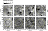 |
Fig. 2 Average (stacked) images of the apparent vortex area in HMI (top row) and Hα −1.03 Å (bottom row) for certain similar time intervals. The first column shows an average image of the entire observed second time series, while the other columns show average images for shorter time intervals within the second time series that are denoted within each image. The overplotted yellow circle indicates the location of the analysed conspicuous vortex flow as seen in Hα . |
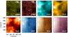 |
Fig. 3 Average (stacked) image of the apparent vortex area in all observed AIA channels mapping increasing temperatures within atmospheric layers from the photosphere to the corona. Averaging has been performed over the entire observing interval of 07:32 UT–08:34 UT for the 1600 Å and 1700 Å channels and 07:32 UT–09:16 UT for all other AIA channels (see Sect. 2). The overplotted yellow circle indicates the location of the analysed conspicuous vortex flow as seen in Hα. |
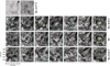 |
Fig. 4 Indicative images of the conspicuous vortex flow (yellow circle) at different times and wavelengths of the Hα line. Red, green, cyan, and orange circles mark the smaller observed swirls discussed in Sect. 3.2 that exhibit different morphological structures and patterns. The temporal evolution of the vortex flow in Hα line-centre intensity is shown in the left panel of the movie available online. |
In the Ca II 8542 Å line the picture is somewhat different to that of Hα (third row of Fig. 1, and Fig. 5). Although chromospheric swirls were first observed in the Ca II 8542 Å line (see references in Sect. 1), the conspicuous Hα vortex flow is not seen at all, even at the Ca II 8542 Å line centre (cf. Fig. 5c and the corresponding Hα image in Fig. 4g). This may suggest that the vortex flow seen in the Hα line-centre and near line-centre wavelengths lies higher than the formation height of the Ca II line centre. The latter, according to the three-dimensional non-local thermodynamic equilibrium (non-LTE) radiative transfer computations of Leenaarts et al. (2009) is formed at ~1 Mm above the photosphere (see their Fig. 4), while the Hα line centre is formed at ~1.5 Mm (almost 0.5 Mm higher, see Fig. 4 of Leenaarts et al. 2012) with some significant contributions also from lower heights close to 0.4 Mm. Even Hα ± 0.26 Å, where the vortex flow is also clearly seen (see Fig. 4), seems to mostly form above the Ca II 8542 Å line centre. However, what is also seen in the Ca II 8542 Å line-centre and near line-centre wavelengths, i.e. ±0.055 Å and ±0.11 Å, is the vortex substructure (see Fig. 5, panels a–e) seen also in the Hα line-centre and near line-centre wavelengths and discussed in Sect. 3.2. This most probably suggests that these substructures are lying at the formation height of the Ca II 8542 Å line-centre and near line-centre wavelengths, below the apparent vortex flow height. Furthermore, we can also see in the Ca II 8542 Å line extreme blue wing upflow events similar to those seen in Hα (see Fig. 5f which depicts the same upflow event seen in Hα in Fig. 4v).
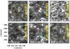 |
Fig. 5 Indicative images of the ROI, almost co-temporal with respective Hα images of Fig. 4, at different wavelengths of the Ca II 8542 Å line. The yellow circle denotes the area of the conspicuous Hα vortex flow (e.g. Fig. 4g) while red, green, and orange circles denote smaller observed swirls also seen in Hα (see panels of Fig. 4) and discussed in Sect. 3.2. The white rectangle in panel f encloses the upflow event also seen in the extreme Hα blue wing (Fig. 4v). |
Similarly to Hα , individual swirls are also simultaneously seen in blue and red near line-centre Ca II wavelengths, due to the opacity of these absorbing structures. They are much clearer in the blue wing because of a significant upwards velocity contribution to the respective line intensity. Generally, similar structures are thicker and sharper in Hα than in Ca II 8542 Å, due to differences in the formation mechanism of these lines and thus in the rendering of the chromosphere (see for an interesting comparison and discussion about the formation of these two lines Cauzzi et al. 2009). The detection of swirls in Ca II is mostly possible only by direct comparison with the corresponding Hα vortex flow images.
3.1.2. Vortex flow in SDO/HMI and SDO/AIA channels
The HMI magnetograms do not indicate the presence of strong magnetic flux concentrations within the apparent vortex flow area. Inspection of the HMI time series (indicative images are shown in Fig. 2, first row) reveals very low magnetic fields in this region, within the ~20–30 Gauss HMI uncertainty, with a very noisy temporal behaviour. However, at certain time intervals, low magnetic flux concentrations systematically appear at specific (although variable with time) locations within the vortex area. Amplitude-wise, they are still below the HMI uncertainty, but they do imply the appearence/existence of a magnetic structure. Comparison of HMI images with the respective Hα −1.03 Å far blue-wing images (far red-wing images are similar) in Fig. 2, second row, does not reveal any particular association between magnetic field concentrations and Hα BPs that are usually related to small-scale magnetic elements with field strengths ≫100 G and often up to kG levels. The same holds for both Ca II wings. Only the low spatial resolution 1600 Å and 1700 Å AIA channels indicate a faint co-spatial intensity enhancement. As the BP intensity contrast increases quickly with the magnetic field (Riethmüller et al. 2014) but does not strongly depend on their diameter, the absence of any associated Hα BPs with the observed magnetic flux concentrations in the low spatial resolution HMI images suggests the existence of either very low spatially diffused magnetic fields or some spatially unresolved kG-strength fields. The latter possibility, although rather unlikely, cannot be convincingly excluded from the present observations. Strong fields within unresolved BPs with diameters much lower than the Hα spatial resolution would only show a weak magnetic flux signature in HMI and possibly some intensity enhancement in the low-temperature AIA channels.
The SDO/AIA observations allow the investigation of the response of the atmospheric layers above the chromosphere up to the corona to the vortex flow. The average (stacked) temporal images of the apparent vortex flow area in eight AIA channels (see Fig. 3) indicate that the vortex flow may have a corresponding response seen up to the Fe XVI 355 Å passband that is detected as an intensity decrease (dark patch) within the vortex area. There is nothing clearly noticeable higher up in the Fe XII 193 Å, Fe XIV 211 Å channels. This EUV dark patch is for low temperature channels smaller than the Hα vortex flow area (yellow circle), but never exceeds its size; it seems to expand in size and move slightly towards the north-east with increasing temperatures and roughly higher atmospheric layers.
The corresponding time series of the observed AIA channels indicate a rather dynamic behaviour. The intensity, which on average remains lower than in adjacent regions (see Fig. 3 and above), fluctuates with time within or close to the area of the apparent vortex, especially for channels corresponding to the transition region and low corona temperatures. However, these temporal variations cannot be directly linked to the respective dynamics observed in the Hα or the Ca II 8542 Å line due to the ten-times lower resolution of the AIA observations.
Although there is always some doubt concerning the relation of this dark patch to the Hα vortex flow (despite their co-alignment), we must note that it is similar to the intensity absorption detected as a signal of chromospheric swirls in SDO/AIA channels by Wedemeyer-Böhm et al. (2012). However, they also reported higher intensities in AIA channels on the periphery of the apparent vortices in Ca II 8542 Å and in the edges of the ring fragments, which are not observed in our case. It is unclear whether this latter difference stems from the absence of associated BPs, contrary to the observations of Wedemeyer-Böhm et al. (2012) where such an association clearly exists. The lower intensities we observe are also reminiscent of the dark cavities observed in larger scale long-lived tornadoes (see e.g. Li et al. 2012) that are generally co-located with barbs in filaments/prominences along polarity inversion lines, although no circular brightening is observed around them.
If the observed AIA intensity depletion is related to the observed vortex flow, it would imply that all atmospheric layers within or close to its location (yellow circle) are somehow connected by a coherent structure that expands with height, which never exceeds the size of the area of the Hα vortex flow and starts tilting from the transition region and higher. Although no BPs are seen within the vortex area either at the Hα or Ca II wings, which could point to magnetically driven swirling motions (as suggested by Wedemeyer et al. 2013 and Wedemeyer & Steiner 2014), this apparent expansion with height resembles the expansion of magnetic structures widely observed at the Sun.
3.2. Characteristics and substructure of the vortex flow
The Hα vortex flow, clearly seen in Fig. 4 (yellow circle), has an almost circular shape with a radius of ~3″ and a variable centre around position (x, y) = (124.8″, −592″). The vortex size is larger than the majority of those previously observed and reported in Ca II Hα (Bonet et al. 2008), Ca II 8542 Å (Wedemeyer-Böhm & Rouppe van der Voort 2009), Fe I 5250.2 Å (Bonet et al. 2010), or even Hα (Park et al. 2016), which have a radius of ~0.5″–2″. It is only comparable with the mean radius of 2″± 0.7″or the radius of individual swirls observed by Wedemeyer-Böhm et al. (2012) in Ca II 8542 Å (see their supplementary Table 1). In addition to its impressive size, the most striking characteristics are its persistence and long duration, as it is clearly visible during almost the entire observational interval, i.e. for ~100 min. This is far longer than any duration reported so far (usually in the range of 5–16 min) for small-scale vortices or individual swirls (e.g. Bonet et al. 2010; Wedemeyer-Böhm et al. 2012). The conspicuous rotation of the vortex flow is clockwise as we will further analyse below (see also movie attached to Fig. 4).
A closer examination of the entire 1.7 h Hα time series reveals the presence of at least four smaller swirls within or adjacent to the conspicuous large vortex flow. Their approximate location is roughly denoted by red, green, cyan, and orange circles in Fig. 4, while their exact location centroid and shape varies greatly with time. Three of these swirls, marked by red, cyan, and orange circles in Fig. 4, are clearly visible at certain time intervals during the entire time series. The presence of the fourth swirl, marked by a green circle in Fig. 4, is mostly revealed through its interaction with nearby fibril-like structures as their material is forced to twist and follow the swirling flow. All these swirls are not always visible during the entire time series, but they are intermittent and reappear around the same location. Their durations (of the order of a few minutes) and sizes match those previously reported in the literature for chromospheric swirls.
In particular, the swirl marked by a red circle is the most regular one, with its centroid coinciding with the centroid of the conspicuous large vortex flow (yellow circle) and when clearly observed seems to rotate clockwise. This is probably the core swirl of the large vortex flow. The swirl marked by a green circle, lying on the northwest border of the large vortex flow is the most irregular one as it is barely noticeable and only indirectly, as already noted above (see Figs. 4b, i, j, and p). Its low observability probably stems from its close proximity to a chain of overlying fibril-like structures that cover the area most of the time. This rare and small swirl seems to rotate anticlockwise. The swirl marked by a cyan circle is the most intriguing one and like the swirl marked by a red circle seems to be intermittent but quite regular. Most of the time its centroid is just outside the conspicuous large vortex flow at its south-west border (see Figs. 4c, d, and r); however, at times it seems to move inside it (see Fig. 4k). It is mostly rotating anticlockwise, but sometimes its rotation changes to clockwise. Just like the swirl marked by a green circle, at times it interacts with nearby fibril-like structures and twists their material flow (see Fig. 4o). This swirl has been thoroughly analysed by Park et al. (2016), but only for a few minutes during the first part of the observed time series. The swirl marked by an orange circle is the most rarely observed one, briefly visible for a few time intervals (see Figs. 4n, q, and u) within the large vortex flow close to its south-east region and seems to rotate clockwise. It is, however, not clear whether it is really an independent swirl or rather the same as the swirl marked by a red circle with its centroid location largely displaced.
It should be noted that the locations of the swirls marked by a red and cyan circle coincide with the locations of the magnetic flux enhancements that are observed in HMI (see Fig. 2) with the flux enhancement associated with the latter being much stronger. However, as already mentioned, there seem to be no notable BPs observed in Hα or Ca II 8542 Å associated with these HMI magnetic flux enhancements, but only a faint intensity enhancement in the 1600 Å and 1700 Å AIA channels associated with the location of the swirl marked by a cyan circle.
In the Ca II 8542 Å line (see Fig. 5 for indicative snapshots), most of the individual swirls are sometimes visible simultaneously with the corresponding Hα swirls, but usually as small, much fainter, and less thick dark patches and with a small spatial offset. In particular, the swirl marked by a red circle is notably the most visible one in line-centre and near line-centre Ca II wavelengths, following our previous suggestion that this is probably the core swirl of the large vortex flow. The swirls marked by the green and orange circles are hardly visible and are rarely observed compared to the swirl marked by the red circle, while the swirl marked by the cyan circle is not seen at all. This indicates that this swirl probably lies above the formation height of the Ca II 8542 Å line. This is also suggested by its noted interaction with nearby Hα fibril-like structures, which are not seen in the respective Ca II 8542 Å images.
The smaller size of the central swirl observed in the Ca II 8542 Å line compared to the larger size of the Hα conspicuous vortex flow fits the big picture of vortices being magnetically rotating structures whose diameters increase with height as a result of the decrease in the gas pressure balancing the magnetic pressure of the structure. The result is a funnel-like rotating structure, as also indicated by its area expansion in AIA channels.
It is not clear whether the aforementioned smaller swirls are manifestations of the intricate substructure of the large vortex flow itself or separate individual swirls that form and appear intermittently within and around the large conspicuous vortex flow. Swirls are thought to rotate approximately as rigid bodies (Wedemeyer-Böhm et al. 2012); however, this is probably not exactly the case. Any deviations from this uniform quasi-rigid body rotation in neighbouring layers of the vortex flow, induced by internal (e.g. waves) or external (e.g. nearby structures) factors, could create instabilities, and thus the temporal appearance of smaller eddies or vortices. Fedun et al. (2011b), for example, using full non-linear three-dimensional magnetohydrodynamic simulations of a vortex-driven magnetic flux tube, have shown that the twisting of an open flux tube by photospheric vortices leads to the formation of swirling patches higher in the atmosphere due to the spatially dependent frequency filtering of generated torsional Alfvén waves. The presence of waves in the vortex region will be extensively analysed in a future work.
The morphology of the conspicuous vortex flow and of the individual swirls in Hα includes all schematic patterns reported in literature to date (see Fig. 3 in Wedemeyer-Böhm & Rouppe van der Voort 2009, for an overview). The observed swirl patterns vary with time; occasionally rings (Figs. 4l and p), ring fragments (Figs. 4v and w), spirals (Figs. 4s and t), and spiral arms/arcs (Figs. 4j, m and t) are present. Sometimes more than one of these patterns can be seen. The observed swirl patterns are highly variable, with the exception of arcs that are visible for longer times. They fade away and reappear as a result of variable visibility also caused by nearby flows in the area and/or interactions with them. In the Ca II 8542 Å line, structures are not as clear as in Hα (see Fig. 5); mostly rings, ring fragments, and spiral arms/arcs are occasionally seen as parts of the smaller swirls.
Furthermore, in agreement with previous observations and simulations, lanes composed of leading bright rims and trailing dark edges are present (see Fig. 6) in underlying and nearby granules both in Hα and the Ca II 8542 Å line, which are considered a visible signature of horizontally oriented vortex tubes (Steiner et al. 2010). Our observations in both lines indicate the presence of such structures also in the blue wing, apart from the red wing where they have been examined in those observations and simulations. This suggests that the formation of such rims and edges, which has been mainly attributed to velocity, also has a significant contribution from opacity and temperature.
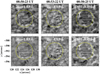 |
Fig. 6 Indicative Hα and Ca II 8542 Å images at two extreme wing wavelengths indicating the positions (white rectangles) of the leading bright rims and trailing dark edges within the conspicuous vortex flow (yellow circle) discussed in Sect. 3.2. |
3.3. Doppler velocities
Figure 7 shows indicative maps of the derived Doppler velocities illustrating vortex-related patterns, such as rings, ring fragments, spirals, and spiral arms/arcs, as also seen in the respective intensity images (see Fig. 4). These patterns are clearly associated with upwards velocity motions (negative Doppler velocities) with a velocity amplitude up to ~8 km s−1, similar to the value derived by Park et al. (2016). A better overview of these upwards motions is provided in Fig. 8 (top panel), which shows the mean upwards Doppler velocity of vortex-related patterns within the conspicuous vortex flow area as a function of time. These upwards-moving structures are identified in each intensity image as absorbing (dark) structures with a line-centre intensity below a certain count threshold. The count threshold is variable with time as it is corrected for intensity variations (e.g. due to seeing effects) that are derived from the average line-centre intensity variation of the entire ROI. The derived upwards velocities, with an overall mean value of −2.9 ± 0.7 km s−1, when taking into account respective errors and projection corrections, as the centre of the ROI lies at a latitude ~38° south of the solar equator and a longitude of ~10° west of the central meridian, are within the reported in literature values (e.g. Wedemeyer-Böhm & Rouppe van der Voort 2009). The respective area occupied by vortex-related upwards moving structures (see Fig. 8, bottom panel) also varies with time around an overall mean value of at least 24.2 ± 8.4%, as this obviously depends on the above-mentioned selected count threshold. We note that this threshold-dependence for the derived Doppler velocities is rather weak, while variations in both quantities do not depend on the chosen threshold. Both the amplitude of Doppler velocities and the respective vortex-structure areas increase with time and are higher during the second part of the observations, reflecting a vortex flow that is much richer in structure, even visually.
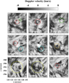 |
Fig. 7 Indicative images of the Doppler velocities derived from the Hα profiles as explained in Sect. 2. Negative and positive Doppler velocities indicate respectively upwards and downwards LOS motions. The yellow circle denotes the conspicuous vortex flow while red, green, cyan, and orange circles (see also Fig. 4) denote smaller observed swirls (see Sect. 3.2). The temporal evolution of Doppler velocity is shown in the right panel of the movie attached to Fig. 4. |
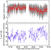 |
Fig. 8 Top panel: variations in mean upwards Doppler velocity (red diamonds) of vortex-related structures within the conspicuous vortex area (yellow circle in Figs. 1 and 4) and their respective errors (standard deviation, grey lines). Bottom panel: percentage of the conspicuous vortex area (yellow circle in previous figures) that is occupied by the identified upwards-moving vortex-related structures as a function of time, used for the derivation of the mean upwards Doppler velocity presented in the top panel. |
3.4. Dynamics
In order to better understand the dynamics of the vortex flow we investigate temporal variations in intensity in both lines and Doppler velocity in Hα along horizontal and vertical slits in the respective two-dimensional image time series (time-slice images). As the large vortex flow shows several intermittent swirls (see Sect. 3.2), we investigate two of them (marked by red and cyan circles in Fig. 4), for specific time ranges when the respective swirl is clearly visible. In order to enhance visibility in both chosen Hα and Ca II intensity images (line centre and −0.055 Å, respectively), we have applied unsharp masking by subtracting the corresponding smoothed image obtained with the Interactive Data Language (IDL) SolarSoft procedure filter_image.pro (using its default values) from each image of the time series. Figures 9 and 10 show time-slice images in Hα and Ca II, respectively, for the same swirls, locations, and time ranges. Although, as already pointed out in Sect. 3.2, the respective swirl centres generally do not exactly coincide in the two lines, our choice of common slits makes comparison between them easier.
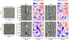 |
Fig. 9 Unsharp-masked (see text for details) Hα line-centre intensity images (first column) and corresponding time-slice Hα line-centre intensity and Doppler velocity images along the horizontal (Cols. 2 and 3, respectively) and the vertical (Cols. 4 and 5, respectively) slits shown in the first column images as green lines. The two slits pass from the approximate visual centres of the chosen swirls, marked by red and cyan circles in Fig. 4. The yellow circle in the first column images and the yellow vertical lines in the time-slice images indicate the borders of the conspicuous vortex flow; vertical green lines on the time-slice images show the approximate centre position of the respective swirl, while horizontal white lines indicate the time corresponding to the image shown in the first column. In velocity time-slice images negative and positive Doppler velocities indicate upwards and downwards LOS motions, respectively. |
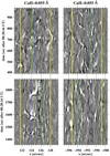 |
Fig. 10 Time-slice Ca II−0.055 Å intensity images derived from the respective unsharp-masked images (see text for details) along the same horizontal (Col. 1) and vertical (Col. 2) slits shown on the unsharpmasked Hα intensity image of Fig. 9 (Col. 1) as green lines. The slits pass from the same approximate visual centres of the chosen swirl marked by a red circle (Row 1) and the swirl marked by a cyan circle (Row 2) of Fig. 9. The yellow vertical lines indicate the borders of the conspicuous vortex flow, while vertical green lines show the approximate centre position of the respective swirl. |
As the dynamics in Hα of the central swirl marked by a red circle indicate (top row of Fig. 9), there is a completely different dynamical behaviour inside and outside the borders of the vortex flow that seems to be similar along the two investigated directions. However, the vortex dynamics is sometimes affected by the presence and dynamical behaviour of fibril-like structures (see Fig. 1 and left panel of the movie attached to Fig. 4) in the upper right part of the vortex flow that corresponds to the right part of all time-slice images. These structures are mostly clearly seen outside the borders of the vortex as dark (absorbing) intensity features or as downflows in Doppler velocity time slices (e.g. top left panel of Fig. 9 along the horizontal slit for times above 600 s). Sometimes, however, as in this particular case, they penetrate well inside the respective vortex flow borders (indicated by the vertical yellow lines) perturbing the vortex dynamics further. In the Ca II 8542 Å line (see Fig. 10) the vortex flow clearly does not extend to the borders of the Hα vortex flow, but is spatially limited closer to its centre, in line with the morphological description provided in Sect. 3.2.
The unsharp-masked Hα intensity images (Fig. 9) show several spiral arms starting from the centre of the two swirls, seen as alternating dark and bright features propagating outwards in opposite directions for several minutes. This propagation seems to be facilitated for both swirls along the south–north direction (vertical slit) as there is clearly more spiral structure along the corresponding time slices than the respective horizontal ones. Furthermore, we note that the outward propagation is not linear as there is clearly a complementary swinging motion with time that is present almost everywhere in our ROI and within the vortex area. The presence of this oscillatory behaviour at every location within the vortex flow with time is probably suggestive of a rigidly or quasi-rigidly rotating vortex structure. From the linear-trend of the expansion of the outmost spiral features in the intensity images along the vertical slit we can estimate an expansion velocity of the order of 3 km s−1. This is slightly lower than the expanding motion of 4–6 km s−1 derived for a small-scale Hα swirl by Park et al. (2016). The derived expansion velocity mostly pertains to the visual expansion of the structure itself (i.e. of its spirals if it could be roughly described by a logarithmic spiral). Therefore, it should not be confused with any horizontal vortex flow velocities derived in literature (e.g. simulations by Moll et al. 2011a; Wedemeyer-Böhm et al. 2012). However, the possibility of any superimposed horizontal velocity components stemming from other present flows in this dynamic quiet-Sun region cannot be excluded. At this point, it is worth mentioning that Wedemeyer-Böhm et al. (2012) estimated radial velocities at the formation height of the Hα line centre of ~10−12 km s−1.
The corresponding Hα Doppler velocity slices in Fig. 9 provide a rather different and somewhat confusing behaviour for the two swirls. While the swirl marked by a red circle (top row) shows both downwards and upwards motion with time, the swirl marked by a cyan circle is associated mostly with downwards motions. There are some temporal instances where alternating upwards and downwards motions follow the different, present spiral arms with the most notable one for the swirl marked by a cyan circle (second row of Fig. 9 along the vertical slit and for the temporal range of 1430–1580 s).
The time-slice Ca II intensity images (Fig. 10) are very different to the respective Hα images in line with the differences between the two lines already described in previous sections (see Sect. 3.1.1). The richness of outward moving spiral arms observed in Hα is not present at all. There are only faint signatures of them, mostly visible for the swirl marked by a cyan circle (bottom row) rather than within the swirl marked by a red circle (top row) and in any case very close to the swirl centre.
We note that in the intensity Hα time slices (see also left panel of movie attached to Fig. 4), at specific locations within the apparent vortex area (top row of Fig. 9) there are some persisting dark features appearing, due to unsharp masking, as featureless regions (e.g. at x = 122″–123.5″ and at y = −594.5″ to −593″). These features, when looking at the entire time series, are present at the end of the first observing interval and the beginning of the second one. Their exact location varies slightly with time and their intensity also seems to be modulated by oscillations within the vortex. It is not clear whether these persistent dark structures represent static vortex-related spiral arms and arcs or material from overlying and nearby structures trapped by the overall vortex flow. Only some very faint signatures of such features are observed in the Ca II 8542 Å line, but for shorter time intervals than in Hα , indicating that these features mostly reside higher than the formation height of the Ca II 8542 Å near line-centre wavelengths.
In order to better understand the behaviour of the Hα vortex flow and check whether it could be described by a rigidly rotating logarithmic spiral as in the work of Bonet et al. (2008) and more recently in the work of Mumford & Erdélyi (2015), we have used a toy model of a clockwise rotating logarithmic spiral with an imposed arbitrary swinging motion that is shown in Fig. 11. The resulting time slices, shown in Fig. 11b, exhibit similar, concave, outward-propagating swinging structures, corresponding to the spirals of the vortex, just like those seen in the time-slice images (see Fig. 9 and its description above). We should note that in the absence of a swinging motion these structures would simply be concave. However, in time slices derived from observations these structures do not appear regular and symmetric to the vortex centre as they do in the toy model, indicating that either this vortex is not precisely an ideal logarithmic spiral or that even if at times it starts as one, it is then highly perturbed by internal (e.g. waves) or external (e.g. nearby flows) forcing.
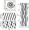 |
Fig. 11 Toy model of a clockwise rigidly rotating logarithmic spiral with a swinging motion. Panel a: snapshot of the logarithmic spiral with the red circle denoting the circular slit used for the time-angle slices of panels c and d with the clockwise angle defined as in Fig. 12 (panel b). The arrow indicates the direction of the imposed swinging motion. Panel b: time-slice image along the green horizontal slit of panel a. Panel c: time-angle slice along the circular red slit of panel a with the swinging motion inhibited. Panel d: same as panel c, but with swinging motion. In all panels we have used arbitrary spatial and temporal units while the logarithmic spiral has been rotated six times with a rotational period T rot. |
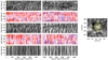 |
Fig. 12 Panel a: time-slice images of Hα −0.26 Å intensity (black and white images) and derived Doppler velocities (coloured images) along circular slits of different radius r (in ″) from a common centre at (x, y) = (124.8″, −592″), such as the one shown in the Hα −0.26 Å image of panel b. The X-axis represents time running from the start of the observations and the Y-axis denotes the angle in degrees at the centre of the circle that is subtended by the arcs starting at the west of the image and measured in the clockwise direction. In intensity time-slice images black indicates absorbing features, while negative and positive Doppler velocities indicate respectively upwards and downwards LOS motions (the Doppler velocity scale is similar to that in Fig. 9). Panel b: indicative Hα −0.26 Å image with the circular slices of increasing radius and respective clockwise angles used for the time-slice images of panel a marked on it. |
Another way to analyse the intricate dynamics of the whole apparent vortex flow, rather than that of the individual swirls, is by constructing time-angle slice images taken along circular slits of different radius r from the centre of the conspicuous flow, as shown in panel a of Fig. 12 and in Fig. 13, with the angle measured in a clockwise direction as indicated in Fig. 12b. Clockwise rotating absorbing structures, such as the upwards moving spirals of the vortex, should appear both in intensity and Doppler velocity time slices as acute-angle propagating structures and this is clearly the case. The vortex-related activity is seen in Hα intensity and Doppler velocity time slices (see Fig. 12) for the entire ~1.7 h duration of our observations. However, it seems to be more evident and to exhibit more structure after the second half of the first observing interval (i.e. after ~1500 s). This behaviour also roughly holds for the Ca II 8542 Å intensity slices (Fig. 13). Comparison of the Hα Doppler velocity time-angle slices with the respective (or nearby) Hα intensity ones shows a less confusing picture for the vortex flow pattern than the time slices of individual swirls in Fig. 9. They are qualitatively similar, at least within the vortex boundaries, indicating that very dark (absorbing) intensity features, as already noted before, are clearly mostly associated with upflows.
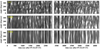 |
Fig. 13 Time-slice images of Ca II−0.055 Å intensity along circular slits of different radius r (in ″) from a common centre at (x, y) = (124.8″, −592″), such as the one shown in panel b of Fig. 12. Black indicates absorbing features. For a description of the axes see the caption of Fig. 12. |
In the Ca II 8542 Å line (see Fig. 13) the vortex flow is limited within radii of ~1″ while in Hα it extends to radii of at least 2″, suggesting a funnel-like expansion of the vortex structure with height. Furthermore, this difference in the appearance and behaviour of the vortex flow in the two lines does seem to suggest the presence of a central vortex driving. Even the behaviour of the time-angle slices for the same line with increasing radius from the centre and particularly the more uniform pattern observed near the centre that gets more complicated and structured as we move radially outwards, is indicative of such a central engine that powers the whole vortex flow. This is in line with suggestions already made in Sect. 3.2 about the swirl marked by a red circle that is mostly located around the vortex flow centre.
In time-angle slices closer to the centre (i.e. r = 0.2″), in both lines, vortex-related structures show a complete rotation. However, further out (i.e. r ≥ 1″), complete rotation is clearly disrupted a) by some persisting (with time) dark features (e.g. at an angle ~ 200°) as noted before, b) by the presence and dynamical behaviour of fibril-like structures for angles in the range of ~270°−360°, or c) some other internal or even external forcing (see also below). However, it should be noted that the qualitatively similar behaviour between time-angle slices for different radii is suggestive of a rigidly or quasi-rigidly rotating structure.
The toy model in Fig. 11 demonstrates the behaviour of the vortex flow as if it were a rigidly clockwise rotating logarithmic spiral structure. The constructed angle-time slices of panels c and d, respectively without and with imposed swinging motion, indicate similar patterns to those seen in the respective figures derived from observations in Figs. 12 and 13. Their comparison indicates that close to the centre of the flow (r = 0.2″) the observed behaviour is clearly more like the case of a non-swinging rotating logarithmic spiral, or at least one exhibiting less enhanced swinging with decreasing radii as even close to the centre there is still at times signatures of such swinging motions (e.g. Fig. 12 around 1000 and 5700 s). Furthermore, it suggests that possibly the swinging motion could be another driver/component for the more complicated patterns seen in time-angle slices as we move radially outwards.
Comparisons between the toy model and the observed timeangle slices, particularly for the less disrupted pattern observed for r = 0.2″ in both lines, also provide a rough first estimate of the rotation period of the vortex structure which seems to be in the range from 200 to 300 s. This period is much lower than the 35 min period reported by Bonet et al. (2010); however, it is within the range of swirling periods derived from simulations by Moll et al. (2011a). A more detailed study of oscillatory and rotational periods will be provided in a future paper.
4. Discussion and conclusions
We have analysed a two-part 1.7 h time series (with a 7 min interval) of a vortex flow simultaneously seen in a) high temporal and spatial resolution CRISP observations in several wavelengths of the Hα and Ca II 8542 Å lines covering the photosphere and chromosphere, b) SDO/HMI LOS photospheric magnetograms, and c) several channels of SDO/AIA covering solar atmospheric temperatures/heights from the upper photosphere to the corona. For the Hα line that has a regular wavelength coverage along its profile, Doppler velocities have been also derived and analysed. Observations in Hα line-centre and near line-centre wavelengths reveal the existence of a clockwise rotating vortex flow, which in addition to its impressive size (comparable with some of the largest swirls reported so far in literature), persists (at least) for the entire duration of our observations. Such a long duration has never been seen before at the chromospheric level and is far higher than any value previously reported in the literature for such small-scale vortex structures; it resembles a small-scale quiet-Sun tornado in analogy to persistent giant tornadoes.
The vortex flow appears quite different in the Ca II 8542 Å and Hα wavelengths: clearer, larger, and more structured in Hα than in Ca II 8542 Å reflecting the different formation heights and different responses of the two lines to the dynamics and structure of the chromosphere. As inferred from the dynamics of the vortex flow along intensity and Doppler-velocity time-angle slice images along circular slits of different radius r from its centre, in both lines the vortex flow is more structured mostly during the second part of our time series. However, while in Hα the vortex flow clearly extends to radii larger than 2″, in the Ca II 8542 Å line it is limited only within radii of ~1″. Furthermore, the vortex flow is occasionally clearly disrupted by the presence of nearby flows that sometimes penetrate well within the vortex flow boundaries and is further complicated by the existence of a swinging motion, revealed in time-slice images that could be due to internal forcing (e.g. waves) or to external forcing (e.g. nearby flows). The analysis of Hα Doppler velocities which confirms the above-mentioned temporal behaviour of the vortex flow reveals that absorbing (dark) intensity structures within the vortex flow occupy on average ~25 ± 8% of the vortex area and have a mean upwards LOS velocity of 2.9 ± 0.7 km s−1, with upwards motions sometimes reaching up to 8 km s−1, well within the reported literature values when also taking into account projection effects. This is further complemented by the comparison of respective time-angle intensity and Doppler velocity slices that reveal a correlation between dark absorbing structures (that represent spiral arms or fragments/patterns of the vortex structure) and mostly upwards velocities.
The appearance of the vortex flow in Hα and Ca II 8542 Å images, as well as its behaviour in time-angle slices of different (increasing) radii suggests an apparent expansion of its size with height. This expansion may also be related to the appearance of the vortex flow as a dark (intensity-depleted) expanding patch in different AIA channels with increasing temperature and to some extent formation height, suggesting that the vortex structure probably spans a large height range. Furthermore, it resembles the expansion of magnetic structures widely observed on the Sun; however, no BPs are seen within the vortex area either at the Hα or Ca II wings that could clearly indicate magnetically driven swirling motions. Even the systematic appearance of some magnetic flux concentrations in HMI LOS magnetograms does not imply a magnetically driven structure as suggested by Wedemeyer et al. (2013) and Wedemeyer & Steiner (2014).
Detailed inspection of the vortex flow, particularly in Hα , reveals the existence of significant substructure in the form of several (at least three) intermittent chromospheric swirls, appearing around locations within or adjacent to the large vortex flow, with similar spatial and temporal characteristics to those previously reported in the literature. These individual swirls that exhibit different and sometimes alternating senses of rotation, show morphologically different schematic patterns varying with time: rings, ring fragments, spirals, and spiral arms/arcs. The analysis of the dynamics of some of these individual swirls highlights again the differences already noted between Hα and Ca II 8542 Å. Intensity time-slice images indicate the occasional appearance of several spiral arms starting from the centre of the respective swirls, that are also sometimes clearly visible in Doppler velocity time slices, with a favoured propagation along the south–north direction that is less inhibited by the presence of the nearby fibril-like flows mentioned above. The propagation of these spirals with an expansion velocity of ~3 km s−1 also reveals the existence of a complementary swinging motion which is present in almost the entire ROI and definitely within the vortex. Velocity-wise, different swirls show different dominant Doppler velocity behaviours; the central individual swirl, which is probably associated with the core of the vortex flow, exhibits both upwards and downwards motions.
A toy model of a clockwise rigidly rotating logarithmic spiral with a swinging motion explains the behaviour of several features seen in time slices and time-angle slices concerning individual swirls and the vortex flow as a whole, when compared with respective figures derived from observations. Furthermore, it provides a first rough estimate of the rotation period of the vortex structure that is in the range from 200 to 300 s.
From our present findings, it is not clear whether the observed substructure is indeed composed of individual swirls, forming and appearing recursively within and around the vortex flow or is a manifestation of instabilities in the form of swirling patches within a funnel-like magnetic flux tube driven by the presence of torsional Alfvén waves as indicated by simulations (Fedun et al. 2011b). Further work to examine the possible presence and influence of waves in the vortex region dynamics is obviously needed.
As already discussed, the most striking feature of the large Hα vortex flow is its long duration. Persistent flows of much larger radii have been reported before, as mentioned in the Introduction, in G-band images at supergranular junctions (Attie et al. 2009), and in continuum intensity images and magnetograms (Requerey et al. 2018). In both cases they were clearly connected with magnetic elements. This is, however, the first time that such a small-scale persistent flow is observed and reported for Hα observations and is not connected with any magnetic elements. Providing a clear interpretation for the long duration is rather difficult, due to the complexity and irregularities of the observed 1.7 h flow pattern. It is, for example, unclear whether there is a central swirl acting as an engine for the Hα vortex flow (hereafter, scenario I) or this flow is a result of the combined action of several individual smaller swirls (hereafter, scenario II). In scenario I, the central small chromospheric swirl (swirl marked by a red circle, see Sect. 3.2) could play this vital role. However, it is very intermittent, and thus difficult to grasp how it can drive and then maintain such a persistent vortex flow. On the other hand, the analysed dynamics of the vortex flow (see time-angle slices and relevant description in Sect. 3.4) do suggest the presence of a central vortex. Furthermore, the simultaneous observations of Hα and Ca II 8542 Å at different wavelengths and of different SDO/AIA channels, and thus atmospheric temperatures and heights suggest the presence of a funnel-like structure expanding at least from the photosphere to the low corona. In addition, as mentioned in Sect. 3.4, both the presence of a similar oscillatory (swinging) behaviour at every location within the vortex flow with time and the qualitatively similar dynamic behaviour observed in time-angle slices for different radii is suggestive of a rigidly or quasi-rigidly rotating vortex structure. Although no BPs associated with the vortex flow are observed in Hα and Ca II 8542 Å wing wavelengths, pointing to a magnetically driven structure as suggested by Wedemeyer et al. (2013) and Wedemeyer & Steiner (2014), the possibility of a vortex-flow within a magnetically supported structure cannot be excluded. Scenario II, which involves a combined action of different individual swirls, is even more difficult to understand and, unfortunately, impossible to describe and support with plausible arguments. It should be noted, however, that in scenario I the centralswirl driving of the vortex flow could be assisted by the presence of other nearby swirl motions (swirls marked by the green and cyan circles in this case; see Sect. 3.2) within or adjacent to the vortex flow, and by nearby fibril-like flows. In both scenarios, the vortex flow could also be fed with material from nearby flows as the presence of some persistent absorbing structures clearly suggests (see Sect. 3.4). In conclusion, if scenario I is the prevailing one then we are talking about a swirl of unprecedented duration that has never been accounted for before, both in observations and/or simulations. In scenario II it is even harder to explain the very complicated motion dynamics involved through a descriptive only analysis, not involving relevant simulations, which are beyond the scope of the present work. Below, we refer to another possible scenario (scenario III).
From the discussion above, some pertinent unanswered questions arise. Are there any unobserved sub-resolution (i.e. lower than those achieved with the present CRISP observations) magnetic elements present that are related to these vortex flows? Unfortunately, the lack of any relevant high-resolution magnetograms does not allow a definite answer to this question, while the HMI spatial resolution only points to the existence of some magnetic enhancements that are, unfortunately, not associated with any BPs, either in the Hα or Ca II 8542 Å wings. Is this likely to be a different case of a hydrodynamically driven vortex flow (scenario III) that has not been considered so far in the literature and/or simulations? The size, duration, and vertical extent of the analysed vortex flow could point to a small-scale quiet-Sun tornado, similar to giant tornadoes (mostly associated with twisting footpoints of magnetically supported filaments), but certainly much smaller in size. In this case, the observed substructure could be consistent with a manifestation of instabilities in the form of swirling patches within a funnel-like magnetic flux tube, as mentioned before, at the centre of a supergranule, but driven by a hydrodynamic process also involving interaction with neighbouring fibril-like flows. It is, however, a difficult question to conclusively answer, as small-scale quiet-Sun vortex flows have been mostly observed in Ca lines, G-band, magnetograms, and the respective simulations, with Hα vortex observations only recently grasping our attention (Park et al. 2016). How frequent are such long-duration vortex flows? It is rather difficult to answer this question without analysing several Hα observations. However, from visual inspection there seems to be within our FOV at least one such long-lasting vortex flow, however with a shorter duration, slightly to the north of the ROI.
Our present analysis of the appearance, characteristics, substructure, and dynamics of a persistent vortex flow has already suggested signatures of swinging and/or torsional motions that could result from the presence of relevant waves. The presence of waves and the oscillatory behaviour of the vortex area, which could provide further clues about the intricate structure and dynamics of this long-duration flow, will be studied in a subsequent work.
Movies
Movie of Fig. 4 Access here
Acknowledgments
We acknowledge support of this work from the project “PROTEAS II” (MIS 5002515), which is implemented under the Action “Reinforcement of the Research and Innovation Infrastructure”, funded by the Operational Programme “Competitiveness, Entrepreneurship, and Innovation” (NSRF 2014–2020) and co-financed by Greece and the European Union (European Regional Development Fund). The Swedish 1-m Solar Telescope is operated on the island of La Palma by the Institute for Solar Physics of Stockholm University in the Spanish Observatorio del Roque de los Muchachos of the Instituto de Astrofisica de Canarias. The AIA data are used courtesy of NASA/SDO and the AIA science team. The authors wish to acknowledge the DJEI/DES/SFI/HEA Irish Centre for High-End Computing (ICHEC) for the provision of computing facilities and support. We would also like to thank STFC PATT T&S and the Solarnet project which was supported by the European Commission’s FP7 Capacities Programme under Grant Agreement number 312495 for T&S. Armagh Observatory and Planetarium is grant-aided by the N. Ireland Department of Communities.
References
- Amari, T., Luciani, J.-F., & Aly, J.-J. 2015, Nature, 522, 188 [NASA ADS] [CrossRef] [Google Scholar]
- Attie, R., Innes, D. E., & Potts, H. E. 2009, A&A, 493, L13 [NASA ADS] [CrossRef] [EDP Sciences] [Google Scholar]
- Bonet, J. A., Márquez, I., Sánchez Almeida, J., Cabello, I., & Domingo, V. 2008, ApJ, 687, L131 [NASA ADS] [CrossRef] [Google Scholar]
- Bonet, J. A., Márquez, I., Sánchez Almeida, J., et al. 2010, ApJ, 723, L139 [NASA ADS] [CrossRef] [Google Scholar]
- Brandt, P. N., Scharmer, G. B., Ferguson, S., Shine, R. A., & Tarbell, T. D. 1988, Nature, 335, 238 [NASA ADS] [CrossRef] [Google Scholar]
- Cauzzi, G., Reardon, K., Rutten, R. J., Tritschler, A., & Uitenbroek, H. 2009, A&A, 503, 577 [NASA ADS] [CrossRef] [EDP Sciences] [Google Scholar]
- de la Cruz Rodríguez, J., Löfdahl, M. G., Sütterlin, P., Hillberg, T., & Rouppe van der Voort, L. 2015, A&A, 573, A40 [NASA ADS] [CrossRef] [EDP Sciences] [Google Scholar]
- Fedun, V., Shelyag, S., Verth, G., Mathioudakis, M., & Erdélyi, R. 2011a, Ann. Geophys., 29, 1029 [Google Scholar]
- Fedun, V., Verth, G., Jess, D. B., & Erdélyi, R. 2011b, ApJ, 740, L46 [NASA ADS] [CrossRef] [Google Scholar]
- Jafarzadeh, S. 2013., PhD Thesis, Institut für Astrophysik, Georg-August-Universität Göttingen, Germany [Google Scholar]
- Kitiashvili, I. N. 2014, PASJ, 66, S8 [NASA ADS] [CrossRef] [Google Scholar]
- Kitiashvili, I. N., Kosovichev, A. G., Mansour, N. N., & Wray, A. A. 2012, ApJ, 751, L21 [NASA ADS] [CrossRef] [Google Scholar]
- Leenaarts, J., Carlsson, M., Hansteen, V., & Rouppe van der Voort, L. 2009, ApJ, 694, L128 [NASA ADS] [CrossRef] [Google Scholar]
- Leenaarts, J., Carlsson, M., & Rouppe van der Voor, L. 2012, ApJ, 749, 136 [NASA ADS] [CrossRef] [EDP Sciences] [Google Scholar]
- Lemen, J. R., Title, A. M., Akin, D. J., et al. 2012, Sol. Phys., 275, 17 [NASA ADS] [CrossRef] [Google Scholar]
- Li, X., Morgan, H., Leonard, D., & Jeska, L. 2012, ApJ, 752, L22 [NASA ADS] [CrossRef] [EDP Sciences] [Google Scholar]
- Moll, R., Cameron, R. H., & Schüssler, M. 2011a, A&A, 533, A126 [NASA ADS] [CrossRef] [EDP Sciences] [Google Scholar]
- Moll, R., Pietarila Graham, J., Pratt, J., et al. 2011b, ApJ, 736, 36 [NASA ADS] [CrossRef] [Google Scholar]
- Mumford, S. J., & Erdélyi, R. 2015, MNRAS, 449, 1679 [NASA ADS] [CrossRef] [Google Scholar]
- Mumford, S. J., Fedun, V., & Erdélyi, R. 2015, ApJ, 799, 6 [NASA ADS] [CrossRef] [Google Scholar]
- Park, S.-H., Tsiropoula, G., Kontogiannis, I., et al. 2016, A&A, 586, A25 [NASA ADS] [CrossRef] [EDP Sciences] [Google Scholar]
- Pesnell, W. D., Thompson, B. J., & Chamberlin, P. C. 2012, Sol. Phys., 275, 3 [NASA ADS] [CrossRef] [Google Scholar]
- Requerey, I. S., Cobo, B. R., Gošić, M., & Bellot Rubio, L. R. 2018, A&A, 610, A84 [NASA ADS] [CrossRef] [EDP Sciences] [Google Scholar]
- Riethmüller, T. L., Solanki, S. K., Berdyugina, S. V., et al. 2014, A&A, 568, A13 [NASA ADS] [CrossRef] [EDP Sciences] [Google Scholar]
- Scharmer, G. B., Bjelksjo, K., Korhonen, T. K., Lindberg, B., & Petterson, B. 2003a, in Innovative Telescopes and Instrumentation for Solar Astrophysics, eds. S. L. Keil, & S. V. Avakyan, Proc. SPIE, 4853, 341 [NASA ADS] [CrossRef] [Google Scholar]
- Scharmer, G. B., Dettori, P. M., Lofdahl, M. G., Shand, M., 2003b, in Innovative Telescopes and Instrumentation for Solar Astrophysics, Proc. SPIE, 4853, 370 [NASA ADS] [CrossRef] [Google Scholar]
- Scharmer, G. B., Narayan, G., Hillberg, T., et al. 2008, ApJ, 689, L69 [NASA ADS] [CrossRef] [Google Scholar]
- Scherrer, P. H., Schou, J., Bush, R. I., et al. 2012, Sol. Phys., 275, 207 [Google Scholar]
- Shelyag, S., Keys, P., Mathioudakis, M., & Keenan, F. P. 2011, A&A, 526, A5 [NASA ADS] [CrossRef] [EDP Sciences] [Google Scholar]
- Shelyag, S., Cally, P. S., Reid, A., & Mathioudakis, M. 2013, ApJ, 776, L4 [NASA ADS] [CrossRef] [Google Scholar]
- Stein, R. F., & Nordlund, Å. 2000, in Astrophysical Turbulence and Convection, eds. J. R. Buchler, & H. Kandrup, Annals of the New York Academy of Sciences, 898, 21 [NASA ADS] [CrossRef] [Google Scholar]
- Steiner, O., Franz, M., Bello González, N., et al. 2010, ApJ, 723, L180 [NASA ADS] [CrossRef] [Google Scholar]
- Stenflo, J. O. 1975, Sol. Phys., 42, 79 [NASA ADS] [CrossRef] [Google Scholar]
- van Noort, M., Rouppe van der Voort, L., & Löfdahl, M. G., 2005, Sol. Phys., 228, 191 [NASA ADS] [CrossRef] [Google Scholar]
- Vargas Domínguez, S., Palacios, J., Balmaceda, L., Cabello, I., & Domingo, V. 2011, MNRAS, 416, 148 [NASA ADS] [Google Scholar]
- Wedemeyer, S., & Steiner, O. 2014, PASJ, 66, S10 [NASA ADS] [CrossRef] [Google Scholar]
- Wedemeyer, S., Scullion, E., Steiner, O., de la Cruz Rodriguez, J., & Rouppe van der Voort, L. H. M. 2013, J. Phys. Conf. Ser., 440, 012005 [NASA ADS] [CrossRef] [Google Scholar]
- Wedemeyer-Böhm, S., & Rouppe van der Voort, L. 2009, A&A, 507, L9 [NASA ADS] [CrossRef] [EDP Sciences] [Google Scholar]
- Wedemeyer-Böhm, S., Scullion, E., Steiner, O., et al. 2012, Nature, 486, 505 [NASA ADS] [CrossRef] [PubMed] [Google Scholar]
- Yurchyshyn, V. B., Goode, P. R., Abramenko, V. I., & Steiner, O. 2011, ApJ, 736, L35 [NASA ADS] [CrossRef] [Google Scholar]
All Figures
|
Fig. 1. Top left: SDO/AIA He ii 304 Å image with an overplotted rectangle marking the full FOV of the CRISP observations. Top right: co-temporal full FOV CRISP Hα line centre sample image with an overplotted rectangle marking the ROI. The bottom two rows show the ROI in the seven different wavelengths along the Hα and the Ca II 8542 Å profiles, while the overplotted yellow circle in the line-centre Hα panel indicates the location of the analysed conspicuous vortex flow. |
| In the text | |
|
Fig. 2 Average (stacked) images of the apparent vortex area in HMI (top row) and Hα −1.03 Å (bottom row) for certain similar time intervals. The first column shows an average image of the entire observed second time series, while the other columns show average images for shorter time intervals within the second time series that are denoted within each image. The overplotted yellow circle indicates the location of the analysed conspicuous vortex flow as seen in Hα . |
| In the text | |
|
Fig. 3 Average (stacked) image of the apparent vortex area in all observed AIA channels mapping increasing temperatures within atmospheric layers from the photosphere to the corona. Averaging has been performed over the entire observing interval of 07:32 UT–08:34 UT for the 1600 Å and 1700 Å channels and 07:32 UT–09:16 UT for all other AIA channels (see Sect. 2). The overplotted yellow circle indicates the location of the analysed conspicuous vortex flow as seen in Hα. |
| In the text | |
|
Fig. 4 Indicative images of the conspicuous vortex flow (yellow circle) at different times and wavelengths of the Hα line. Red, green, cyan, and orange circles mark the smaller observed swirls discussed in Sect. 3.2 that exhibit different morphological structures and patterns. The temporal evolution of the vortex flow in Hα line-centre intensity is shown in the left panel of the movie available online. |
| In the text | |
|
Fig. 5 Indicative images of the ROI, almost co-temporal with respective Hα images of Fig. 4, at different wavelengths of the Ca II 8542 Å line. The yellow circle denotes the area of the conspicuous Hα vortex flow (e.g. Fig. 4g) while red, green, and orange circles denote smaller observed swirls also seen in Hα (see panels of Fig. 4) and discussed in Sect. 3.2. The white rectangle in panel f encloses the upflow event also seen in the extreme Hα blue wing (Fig. 4v). |
| In the text | |
|
Fig. 6 Indicative Hα and Ca II 8542 Å images at two extreme wing wavelengths indicating the positions (white rectangles) of the leading bright rims and trailing dark edges within the conspicuous vortex flow (yellow circle) discussed in Sect. 3.2. |
| In the text | |
|
Fig. 7 Indicative images of the Doppler velocities derived from the Hα profiles as explained in Sect. 2. Negative and positive Doppler velocities indicate respectively upwards and downwards LOS motions. The yellow circle denotes the conspicuous vortex flow while red, green, cyan, and orange circles (see also Fig. 4) denote smaller observed swirls (see Sect. 3.2). The temporal evolution of Doppler velocity is shown in the right panel of the movie attached to Fig. 4. |
| In the text | |
|
Fig. 8 Top panel: variations in mean upwards Doppler velocity (red diamonds) of vortex-related structures within the conspicuous vortex area (yellow circle in Figs. 1 and 4) and their respective errors (standard deviation, grey lines). Bottom panel: percentage of the conspicuous vortex area (yellow circle in previous figures) that is occupied by the identified upwards-moving vortex-related structures as a function of time, used for the derivation of the mean upwards Doppler velocity presented in the top panel. |
| In the text | |
|
Fig. 9 Unsharp-masked (see text for details) Hα line-centre intensity images (first column) and corresponding time-slice Hα line-centre intensity and Doppler velocity images along the horizontal (Cols. 2 and 3, respectively) and the vertical (Cols. 4 and 5, respectively) slits shown in the first column images as green lines. The two slits pass from the approximate visual centres of the chosen swirls, marked by red and cyan circles in Fig. 4. The yellow circle in the first column images and the yellow vertical lines in the time-slice images indicate the borders of the conspicuous vortex flow; vertical green lines on the time-slice images show the approximate centre position of the respective swirl, while horizontal white lines indicate the time corresponding to the image shown in the first column. In velocity time-slice images negative and positive Doppler velocities indicate upwards and downwards LOS motions, respectively. |
| In the text | |
|
Fig. 10 Time-slice Ca II−0.055 Å intensity images derived from the respective unsharp-masked images (see text for details) along the same horizontal (Col. 1) and vertical (Col. 2) slits shown on the unsharpmasked Hα intensity image of Fig. 9 (Col. 1) as green lines. The slits pass from the same approximate visual centres of the chosen swirl marked by a red circle (Row 1) and the swirl marked by a cyan circle (Row 2) of Fig. 9. The yellow vertical lines indicate the borders of the conspicuous vortex flow, while vertical green lines show the approximate centre position of the respective swirl. |
| In the text | |
|
Fig. 11 Toy model of a clockwise rigidly rotating logarithmic spiral with a swinging motion. Panel a: snapshot of the logarithmic spiral with the red circle denoting the circular slit used for the time-angle slices of panels c and d with the clockwise angle defined as in Fig. 12 (panel b). The arrow indicates the direction of the imposed swinging motion. Panel b: time-slice image along the green horizontal slit of panel a. Panel c: time-angle slice along the circular red slit of panel a with the swinging motion inhibited. Panel d: same as panel c, but with swinging motion. In all panels we have used arbitrary spatial and temporal units while the logarithmic spiral has been rotated six times with a rotational period T rot. |
| In the text | |
|
Fig. 12 Panel a: time-slice images of Hα −0.26 Å intensity (black and white images) and derived Doppler velocities (coloured images) along circular slits of different radius r (in ″) from a common centre at (x, y) = (124.8″, −592″), such as the one shown in the Hα −0.26 Å image of panel b. The X-axis represents time running from the start of the observations and the Y-axis denotes the angle in degrees at the centre of the circle that is subtended by the arcs starting at the west of the image and measured in the clockwise direction. In intensity time-slice images black indicates absorbing features, while negative and positive Doppler velocities indicate respectively upwards and downwards LOS motions (the Doppler velocity scale is similar to that in Fig. 9). Panel b: indicative Hα −0.26 Å image with the circular slices of increasing radius and respective clockwise angles used for the time-slice images of panel a marked on it. |
| In the text | |
|
Fig. 13 Time-slice images of Ca II−0.055 Å intensity along circular slits of different radius r (in ″) from a common centre at (x, y) = (124.8″, −592″), such as the one shown in panel b of Fig. 12. Black indicates absorbing features. For a description of the axes see the caption of Fig. 12. |
| In the text | |
Current usage metrics show cumulative count of Article Views (full-text article views including HTML views, PDF and ePub downloads, according to the available data) and Abstracts Views on Vision4Press platform.
Data correspond to usage on the plateform after 2015. The current usage metrics is available 48-96 hours after online publication and is updated daily on week days.
Initial download of the metrics may take a while.