| Issue |
A&A
Volume 618, October 2018
|
|
|---|---|---|
| Article Number | A37 | |
| Number of page(s) | 16 | |
| Section | Stellar structure and evolution | |
| DOI | https://doi.org/10.1051/0004-6361/201731701 | |
| Published online | 11 October 2018 | |
Oxygen and helium in stripped-envelope supernovae
1 Department of Astronomy, The Oskar Klein Center, Stockholm University, AlbaNova, 10691 Stockholm, Sweden
e-mail: This email address is being protected from spambots. You need JavaScript enabled to view it.
2 Department of Astronomy, California Institute of Technology, Pasadena, CA 91125, USA
3 Las Cumbres Observatory, 6740 Cortona Dr., Suite 102, Goleta, CA 93117, USA
4 Department of Physics, Broida Hall, University of California, Santa Barbara, CA 93106-9530, USA
5 NASA Goddard Space Flight Center, Mail Code 661, Greenbelt, MD 20771, USA
6 Joint Space-Science Institute, University of Maryland, College Park, MD 20742, USA
7 Department of Astronomy, University of California, Berkeley, CA 94720-3411, USA
8 European Southern Observatory, Karl-Schwarzschild-Strasse 2, 85748 Garching bei München, Germany
9 Miller Senior Fellow, Miller Institute for Basic Research in Science, University of California, Berkeley, CA 94720, USA
10 Benoziyo Center for Astrophysics, Weizmann Institute of Science, 76100 Rehovot, Israel
11 Astronomy Department, University of Washington, Box 351580, U.W., Seattle, WA 98195-1580, USA
12 Racah Institute of Physics, Hebrew University, Jerusalem 91904, Israel
13 Institut für Physik, Humboldt-Universität zu Berlin, Newtonstraße 15, 12489 Berlin, Germany
14 National Optical Astronomy Observatory, 950 North Cherry Avenue, Tucson, AZ 85719, USA
15 Lawrence Berkeley National Laboratory, 1 Cyclotron Road, MS 50B-4206, Berkeley, CA 94720, USA
16 Astrophysics Research Institute, Liverpool John Moores University, IC2 Liverpool Science Park, 146 Brownlow Hill, Liverpool L3 5RF, UK
17 Department of Astronomy, San Diego State University, San Diego, CA 92182, USA
18 Kavli IPMU (WPI), UTIAS, The University of Tokyo, Kashiwa, Chiba 277-8583, Japan
19 Laboratoire de Physique Nucléaire et de Hautes Énergies, Université Pierre et Marie Curie Paris 6, Université Paris Diderot Paris 7, CNRS-IN2P3, 4 place Jussieu, 75252 Paris Cedex 05, France
Received:
3
August
2017
Accepted:
3
July
2018
Abstract
We present an analysis of 507 spectra of 173 stripped-envelope (SE) supernovae (SNe) discovered by the untargeted Palomar Transient Factory (PTF) and intermediate PTF (iPTF) surveys. Our sample contains 55 Type IIb SNe (SNe IIb), 45 Type Ib SNe (SNe Ib), 56 Type Ic SNe (SNe Ic), and 17 Type Ib/c SNe (SNe Ib/c). We have compared the SE SN subtypes via measurements of the pseudo-equivalent widths (pEWs) and velocities of the He I λλ5876, 7065 and O I λ7774 absorption lines. Consistent with previous work, we find that SNe Ic show higher pEWs and velocities in O I λ7774 compared to SNe IIb and Ib. The pEWs of the He I λλ5876, 7065 lines are similar in SNe Ib and IIb after maximum light. The He I λλ5876, 7065 velocities at maximum light are higher in SNe Ib compared to SNe IIb. We identify an anticorrelation between the He I λ7065 pEW and O I λ7774 velocity among SNe IIb and Ib. This can be interpreted as a continuum in the amount of He present at the time of explosion. It has been suggested that SNe Ib and Ic have similar amounts of He, and that lower mixing could be responsible for hiding He in SNe Ic. However, our data contradict this mixing hypothesis. The observed difference in the expansion rate of the ejecta around maximum light of SNe Ic (Vm = √2Ek/Mej ≈ 15 000 km s−1) and SNe Ib (Vm ≈ 9000 km s−1) would imply an average He mass difference of ∼1.4 M⊙, if the other explosion parameters are assumed to be unchanged between the SE SN subtypes. We conclude that SNe Ic do not hide He but lose He due to envelope stripping.
Key words: supernovae: general / stars: abundances / stars: mass-loss / techniques: spectroscopic
© ESO 2018
1. Introduction
Stripped-envelope (SE) supernovae (SNe) are thought to be the result of massive stars undergoing core collapse (CC) after the progenitor stars have been stripped of their envelopes to varying degrees. Among SE SNe there are three main subtypes: Type IIb SNe (SNe IIb), Type Ib SNe (SNe Ib) and Type Ic SNe (SNe Ic). Observationally, the distinction between the subtypes is based on the presence of H and He lines. SNe IIb show helium and hydrogen signatures in early-time spectra, with the hydrogen signatures disappearing over time. SNe Ib show no hydrogen but strong helium features, and SNe Ic show neither hydrogen nor helium lines in their spectra (Filippenko 1997; Gal-Yam 2016). The spectral differences among the SE SN subtypes are typically interpreted as varying amounts of envelope stripping. SNe IIb progenitors would then have undergone partial stripping, retaining a small part of their hydrogen envelopes. SNe Ib progenitors would be fully stripped of their hydrogen envelopes, and SNe Ic progenitors would be fully stripped of both their hydrogen and helium envelopes.
There are two main mechanisms that can give rise to significant envelope stripping: line-driven winds from isolated massive stars (e.g., Conti 1976; Smith 2014) or binary mass transfer (e.g., Iben & Tutukov 1985; Yoon et al. 2010; Claeys et al. 2011; Yoon 2015). However, alternative explanations for the observed subtypes have also been suggested. Enhanced stellar mixing in massive stars could reduce the He envelope mass by burning it into O, which produces SNe Ic with enhanced O abundances (Frey et al. 2013), and differences in the mixing of 56Ni synthesized in the SN explosions could produce SNe of different observational subtypes from progenitors of otherwise similar structure (Dessart et al. 2012). In the models by Dessart et al. (2012), only SN explosions where the synthesized 56Ni is highly mixed throughout the ejecta, so that the He in the envelope can be nonthermally excited, will produce detectable He lines, as seen in SNe Ib. Models with low mixing become SNe Ic. In these models, higher mixing also results in stronger and faster O I λ77741, and thus SNe Ib would show the strongest and fastest oxygen (see Fig. 13 in Dessart et al. 2012).
Observationally, there is some evidence both for and against these scenarios. Piro & Morozova (2014) suggest that up to 1 M⊙of He could sometimes be hidden in SE SNe, as some objects show very low He velocities indicating that the emitting region lies behind a transparent shell (e.g., the Type IIb SN 2010as; Folatelli et al. 2014). In such objects, based on the calculations by Dessart et al. (2012), the 56Ni synthesized in the explosion might only be mixed into a small part of the He envelope, resulting in lower velocities measured from absorption minima, and indicating the possibility that even lower mixing, if possible, could produce no He signatures at all (and thus give rise to SNe Ic with very slow expansion velocities). In contrast to this suggestion, it has been found that SNe Ic on average display the highest velocities, followed by SNe Ib, and finally by SNe IIb at the slowest expansion velocities as measured in both the Fe II λ5169 and the O I λ7774 absorption lines (Matheson et al. 2001; Liu et al. 2016). However, these results were based on a relatively low number of objects, especially for the O I λ7774 line. The SNe included in these studies were also discovered mainly in targeted SN searches.
In this paper, we have performed an analysis similar to that of Liu et al. (2016), in order to check if their results hold with a larger sample. We investigate He I λλ5876, 7065 and O I λ7774 absorption-line strengths and velocities during the photospheric phase for all 176 SE SNe discovered by the Palomar Transient Factory (PTF; Law et al. 2009) and the intermediate PTF (iPTF; Cao et al. 2016; Masci et al. 2017). The PTF and iPTF were untargeted magnitude-limited2 surveys. Thus, our sample should arguably be less biased compared to previous studies of SE SN spectra that have been mostly based on SNe found via targeted searches3. We address the predictions of alternative models for the observed subtypes of SE SNe4, and compare our results to those found by Matheson et al. (2001) and Liu et al. (2016). Our observations are described in Sect. 2. The methods we have used are presented in Sect. 3, and the results are given in Sect. 4. We search for correlations between the various measurements in Sect. 5. A discussion and our conclusions can be found in Sect. 6.
2. Observations and reductions
2.1. Photometry
To estimate the epoch of maximum light for each SN, we used r- or ℊ-band photometry from the Palomar 48 inch (P48) and 60 inch (P60) telescopes, depending on availability for each SN. All photometry has been host-galaxy subtracted. The P60 data were reduced with FPIPE (Fremling et al. 2016), and the P48 data with the PTFIDE pipeline (Masci et al. 2017). The full photometric (i)PTF SE SN sample will be presented in future papers. A subsample has previously been analyzed by Prentice et al. (2016).
2.2. Spectroscopy
During the lifetimes of PTF and iPTF we obtained 507 spectra at unique epochs of SE SNe. We discovered 55 SNe IIb (187 spectra), 45 SNe Ib (125 spectra), 56 SNe Ic (153 spectra), and 17 Type Ib/c SNe (SNe Ib/c; 42 spectra). We have over three times more objects in our sample compared to Liu et al. (2016), who studied 14 SNe IIb, 21 SNe Ib, and 17 SNe Ic. The (i)PTF SE SN spectral sample is summarized in Appendix A.1.
We do not include Type Ic-BL SNe discovered by the (i)PTF in the analysis in this paper; they will be presented by Taddia et al. (in prep.). Hydrogen-poor superluminous SNe (SLSNe) are also excluded. Subsamples of our full spectral dataset have previously been published: some SNe IIb by Strotjohann et al. (2015), iPTF13bvn and PTF12os by Fremling et al. (2014, 2016), iPTF15dtg by Taddia et al. (2016), SN 2013cu (iPTF13ast) by Gal-Yam et al. (2014), PTF12gzk by Horesh et al. (2013), SN 2011dh (PTF11eon) by Arcavi et al. (2011), and SN 2010mb (PTF10iue) by Ben-Ami et al. (2014).
All spectra included in our analysis were reduced using standard pipelines and procedures for each telescope and instrument. The analysis in this paper is focused on the optically thick photospheric phase (we do not analyze spectra taken later than 60 d past maximum light). Normalized spectra limited to the regions around the absorption features used in our analysis will be made available in electronic form via WISeREP5 (Yaron & Gal-Yam 2012). A catalog paper that will present full spectra is in preparation.
3. Data analysis and methods
3.1. Time of maximum light estimates
We estimate the time of maximum light for each SN in our sample using the observed light curves (LCs), by performing template fits to the r-band LC of each object (or the ℊ-band LC if r is not available). When fitting the LCs we allow for a shift and stretch of the templates. The LC peaks of SNe IIb were estimated using the r-band LC of SN 2011dh (Ergon et al. 2014). The LC peaks of SNe Ib and Ic were estimated using the LC templates by Taddia et al. (2015).
The time of maximum light was used to calculate the rest-frame epochs of our spectroscopic observations (see Appendix A.1). Throughout this paper we use the convention that negative epochs refer to epochs before maximum light (e.g., −5 d) and positive epochs refer to past maximum (e.g., +5 d). For objects where it was not possible to determine the time of maximum light, we use the spectra obtained by the (i)PTF to classify them (see Appendix A.1), but do not include them in any further analysis.
3.2. Spectral classifications
To classify the SNe in our sample we have used SNID (Blondin & Tonry 2007) with template spectra constructed from the SE SNe in the Harvard-Smithsonian Center for Astrophysics sample (Modjaz et al. 2014; Liu & Modjaz 2014). The full spectral sequence for each SN has been run automatically through SNID, and the subtype with the most matches across the spectral sequence (before +60 d) is used to classify the SN.
If there are several conflicting matches for different spectra of the same SN, or if there is a similar number of matches for two subtypes for a certain spectral sequence, the results are manually inspected both in SNID and by inspecting the regions around Hα,Hβ, and He I λλ5876, 7065; if the best SNID matches change over time from SNe IIb to SNe Ib, or if both Hα and Hβ absorption is detected at a similar velocity in any early-time spectrum, we classify the object as a SN IIb. Furthermore, if manual inspection is needed, H is undetected, and absorption from both of the He I λλ5876, 7065 lines is detected, we classify the object as a SN Ib; if neither H nor He is detected, the object is classified as a SN Ic (see also Shivvers et al. 2017, who also discuss the difficulty of classifying some SE SNe).
SNe with spectra where the signal-to-noise ratio (S/N) is not sufficiently good to distinguish a SN Ib from a SN Ic, or where the classification remains ambiguous after manual inspection, are classified as SNe Ib/c. These are not included in our analysis, except to check for the impact on average values (Sect. 4) and correlations (Sect. 5) by including these objects in both the SN Ib and SN Ic groups and redoing the calculations. We find no significant changes in any of our conclusions by doing this exercise.
3.3. Pseudo-equivalent widths
To estimate the strength of absorption features in our spectra we utilize the pseudo-equivalent width (pEW; e.g., Nordin et al. 2011), defined as
 (1)
(1)
where λ1 and λN define the estimated extent of the absorption feature ( λ1 < λN), and f0(λi) is the continuum, estimated as a linear fit to the data surrounding λ1 and λN.
We follow similar principles as Liu et al. (2016) when choosing the endpoints of the absorption features and where to measure the continuum levels. First, we smooth the spectrum around the absorption feature. The first peak on the blue side of the feature is then chosen as λ1 and the peak closest to the expected position for the relevant emission-line peak in the rest frame is chosen as λN. The pEW calculation is then performed on the original unsmoothed spectrum. Typical results of this method are shown for an example spectrum taken close to maximum light for each SE SN subtype in Fig. 1 (we show Type Ib iPTF13bvn, data from Fremling et al. 2014; Type IIb SN 2011dh6, data from this work; and Type Ic PTF10osn, data from this work). We note that if there are multiple peaks within ∼100 Å of the apparent ends of the absorption feature, we choose the peaks that give the highest pEW value as λ1 and λN (see feature 1 in the spectrum of SN 2011dh in Fig. 1). In the case where there is no clear peak on the blue side of the absorption feature, we limit the pEW measurement in velocity space to no larger than 25 000 km s−1 for the position of λ1. If there is no clear absorption feature and no clear emission peak to use as λN (typical especially for the He I λ7065 position in SNe Ic), we fix λN at the expected rest-frame position of the emission feature and set λ1 where the value of pEW is maximized while λ1 is below the maximum allowed velocity (see feature 2 in the spectrum of PTF10osn in Fig. 1).
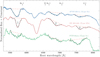 |
Fig. 1. Description of our pEW and expansion-velocity measurement method using spectra around peak brightness for iPTF13bvn (Type Ib, +0.5 d, upper blue line), SN 2011dh (Type IIb, +2.5 d, middle red line), and PTF10osn (Type Ic, +4.0 d, bottom green line). On the spectrum of SN 2011dh, the absorption features of He I λλ5876, 7065 and O I λ7774 have been labeled with numbers. Measurements of features 1–3 have been attempted on all spectra in our sample. For SE SNe, feature 1 is typically associated with He I λ5876, feature 2 with He I λ7065, and feature 3 with O I λ7774, although other elements also contribute to these features. Dashed red lines indicate pseudo-continuum estimates (first-order polynomial fits) for features 1–3 resulting from our measurement scheme (Sect. 3). We calculate pEWs (e.g., Fig. 2) between the endpoints of these continuum estimates using Eq. (1). Velocity estimates are obtained by locating the minima of polynomial fits between the pseudo-continuum endpoints (order 4–7, dashed black lines). If a spectral feature is ambiguous, and has several minima within a similar range as shown for feature 2 in the spectrum of PTF10osn, we set the velocity estimate to be undefined but still calculate the pEW. Wavelengths have been shifted to the rest frame, and the spectra have been normalized and shifted by a constant for clarity. |
Uncertainties in the pEW measurements are estimated using a Monte-Carlo method. First, we create a local measurement of the noise by dividing the original spectrum with a heavily smoothed spectrum and computing the standard deviation locally (in a region of about 1000 Å) around the position of the absorption feature to be measured. Next, we create many simulated noisy spectra by adding noise using a Gaussian distribution and the standard deviation. The pEW measurement is then repeated on each simulated spectrum and the standard deviation of the results is taken as the 1σ uncertainty of our measurements. In this procedure, we also randomly change the continuum endpoints in each simulated spectrum within a 25 Å region to account for possible uncertainties in the identifications of the peak positions of the spectral features. Although this is not necessary for good-quality spectra with accurate peak position estimates, we still perform the same calculation regardless of the spectral quality for consistency7.
3.4. Expansion velocities
To estimate expansion velocities we use the minima of the identified absorption features in our pEW measurements. This is done by fitting a polynomial to the absorption feature and locating the minimum of the fit8. Example fits are shown in Fig. 1 (dashed black lines). Uncertainties are estimated using a similar MC approach as for the pEW measurements. The minimum of each simulated spectrum is estimated by polynomial fits, and the standard deviation is taken as the 1σ uncertainty of our velocity measurements.
4. Results
4.1. Absorption strengths
The method we use to measure pEWs (Sect. 3.3) will by construction tend to give positive values for features 1 and 2 as identified in Fig. 1 for all SE SN spectra, including those of SNe Ic. In SNe IIb and Ib, these features are typically identified as He I λλ5876, 7065. However, positive pEW measurements in a SN Ic does not necessarily mean that He is present in the ejecta. Our method simply maximizes the pEW measurement of any absorption from any line that could give rise to a feature in these regions of the spectrum. Possible contamination for the He I λ5876 absorption line is Na I D, and for He I λ7065, Al II (e.g., Kasliwal et al. 2010). Regardless, throughout this paper we will refer to any measurable absorption found at the position of features 1 and 2 as potential He I λλ5876, 7065 absorption, even for SNe Ic, to simplify the discussion.
4.1.1. Helium
We show the individual He I pEW measurements of the SNe IIb, Ib, and Ic included in our sample in the top panels of Fig. 2. The evolution of the mean values and the standard deviation of the means of each subtype is shown in the middle panels of the figure.
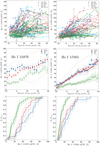 |
Fig. 2. Absorption strengths of He I λ5876 (left panels) and He I λ7065 (right panels). Top panels: individual measurements, with multiple measurements of the same SN connected by solid lines. Middle panels: averages of the SE SN subtypes, with error bars representing the standard deviation of the mean. Dashed lines outline the standard deviations of the samples for each subtype in matching color. Bottom panels: CDFs measured between −10 and +10 d |
Similar to Liu et al. (2016), we find that SNe Ib show larger pEW values on average compared to SNe IIb for the He I λ5876 feature before +20 d, after which the pEW values become similar. The probability that this difference is not real based on a two-sample Kolmogorov–Smirnov (K–S) test is p < 0.03, when we consider the measurements between −10 and +10 days of each subtype. For the same time interval we show the cumulative distribution functions (CDFs) of the pEW values for each subtype in the bottom-left panel of Fig. 2. SNe Ic show significantly weaker absorption in this line at early times (p < 0.001, before +20 d when compared to both our SNe IIb and Ib). However, the pEW values of SNe Ic become more similar to those of the other SE SNe after +30 d. This is likely a result of contamination from Na I gradually becoming more significant, although a weak contribution from He I cannot be ruled out.
In contrast to Liu et al. (2016), we do not find a strong difference between SNe IIb and Ib for the pEW values of the He I λ7065 absorption line at epochs past ∼+40 d (see the middle panels of our Fig. 2 and compare to Fig. 6 in Liu et al. 2016). Instead, we find that SNe IIb and Ib are remarkably similar during all epochs when we could obtain meaningful averages based on measurements of multiple objects (see the bottom-right panel of Fig. 2 for the CDFs for the −10 d to +10 d time interval). In a K–S test we do not find any statistically significant difference among our SNe IIb and Ib in He I λ7065 at any time. Our sample contains several SNe Ib that evolve toward much stronger absorption in this line compared to those studied by Liu et al. (2016). We also have several SNe IIb showing weaker absorption than those studied by Liu et al. (2016). This could be due to the fact that the (i)PTF is untargeted, resulting in a greater diversity of objects, or a consequence of our larger sample size.
SNe Ic show consistently much weaker pEW values measured at the expected position for He I λ7065 absorption at all times, although we do observe a rising trend over time in the pEW values that is similar to that of the other subtypes. This could be evidence for a small residual He envelope in some SNe Ic (but see also Sect. 5.1 and Fig. 5). It could also be due to contamination from the nearby [Fe I] λ7155 line that is gradually getting more significant, or to Al II absorption.
4.1.2. Oxygen
Absorption-strength estimates of the O I λ7774 line are shown in the top panel of Fig. 3. We find that before +20 d, SNe Ic clearly show the highest pEW values, with no detectable difference between SNe IIb and Ib. The pEW distribution we find for SNe Ic is different from both our SN IIb and SN Ib distributions, with p < 0.001 in a two-component K–S test in both cases, when measured in the interval −10 d to +10 d. There is no statistically significant difference between SNe IIb and Ib for any time interval. The evolution of the mean value for each class is displayed in the middle panel of Fig. 3, showing that SNe Ic are on average stronger in this line compared to other SE SNe by almost a factor of two. The CDFs of the subtypes are shown in the bottom panel of Fig. 3. Before peak there are very few SNe IIb and Ib with pEW values higher than 60 Å. Thus, a single pEW measurement of O I λ7774 on an early-time spectrum can be used to classify SNe Ic (see also Sun & Gal-Yam 2017).
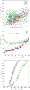 |
Fig. 3. Absorption strengths of O I λ7774. Top panel: individual measurements, with multiple measurements of the same SN connected by solid lines. Middle panel: the averages of the SE SN subtypes, with error bars representing the standard deviation of the mean. Dashed lines outline the standard deviations of the samples for each subtype in matching color. Bottom panel: CDFs measured between −10 and +10 d. |
Past +40 d, there is no statistically significant difference between the pEW values of any of the SE SN subtypes. However, at these later epochs the measurements become difficult owing to increasingly strong emission lines of [Ca II] λλ7293, 7325 that affect the continuum typically used to measure the O I λ7774 absorption. The similarity among the subtypes at later epochs could be a result of this contamination. Table 1 lists the weighted mean pEW for the O I λ7774 absorption feature for each SE SN subtype at maximum light.
Weighted mean values for SE SNe at maximum light.
4.2. Velocities
Typically, the Fe II λ5169 line is used as a tracer for the expansion velocity of the SN photosphere in SE SNe (Dessart & Hillier 2005). The photospheric expansion velocity, measured in this way, can be used for LC modeling (e.g., Arnett 1982), and sample studies of SE SN LCs have in general followed this methodology (e.g., Drout et al. 2011; Cano 2013; Taddia et al. 2015; Lyman et al. 2016; Prentice et al. 2016). However, Dessart et al. (2015) have shown that the notion of a photosphere in SE SNe is ambiguous. Instead, Dessart et al. (2016) suggest that it is more appropriate to estimate the mean expansion rate via the absorption minimum of the He I λ5876 line for SNe IIb and Ib, and the O I λ7774 absorption minimum in SNe Ic. Expansion-velocity measurements based on these lines are presented below (average expansion velocities around maximum light can be found in Table 1).
4.2.1. Helium
Expansion-velocity measurements obtained from the minimum of the He I λ5876 absorption line for the SNe IIb and Ib in our sample are shown in the top-left panel of Fig. 4. For SNe Ic, we find that very few objects show velocities that could be consistent with He I, and there is generally a very large scatter in our measurements (since He is likely not detected). Thus, we do not include results for SNe Ic in this figure or in Table 1.
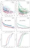 |
Fig. 4. Velocities of He I λ5876 (left panels) and O I λ7774 (right panels). Top panels: individual measurements, with measurements of the same SN connected by solid lines. Middle panels: averages of the SE subtypes, with error bars representing the standard deviation of the mean. Dashed lines outline the standard deviations of the samples for each subtype in matching color. Average velocities derived from He I λ7065 are shown as thick solid lines (Type Ib in blue and Type IIb in red) in the middle-left panel. The average He I λ5876 velocity of Type Ib SNe is shown as a thick solid line in the middle-right panel. Bottom panels: CDFs measured between −10 and +10 d for each subtype. |
SNe Ib tend to be faster, on average, compared to SNe IIb in this line (see the middle-left panel of Fig. 4). Averages obtained from the absorption minimum of the He I λ7065 line (overplotted as thick solid lines in the middle-left panel of Fig. 4) give similar results as for the He I λ5876 line. These findings are consistent with the result by Liu et al. (2016).
Around maximum light the average He I λ5876 absorption velocity of our SNe Ib is ∼9500 ± 600 km s−1. For SNe IIb we measure 8000 ± 500 km s−1. In a two-component K–S test we find that the SN Ib velocity distribution differs from the SN IIb distribution with p < 0.004 for the null hypothesis (calculated between −10 d and +10 d; see also the CDFs in the bottom-left panel of Fig. 4).
4.2.2. Oxygen
Velocity estimates based on the absorption minimum of the O I λ7774 line are shown in the top-right panel of Fig. 4. We find clear evidence for SNe Ic on average being faster compared to SNe IIb and Ib, with a few SNe Ic showing very high velocities at early times, followed by a rapid decline (>18 000 km s−1 before peak; e.g., PTF12gzk; Ben-Ami et al. 2012; Horesh et al. 2013). A similar result was found by Liu et al. (2016). However, their weighted averages at maximum light were based on only 7 SNe Ic and 4 SNe Ib. If we consider the time interval of −2d to 2 d, we have velocity estimates of 14 SNe IIb, 8 SNe Ib, and 22 SNe Ic. In a two-component K–S test for the velocity distributions between −10 d and +10 d, we find that SNe Ic differ from both SNe IIb and Ib with p < 0.01 for the null hypothesis. Even if we exclude the 5 fastest SNe Ic in our sample, we still find a significantly higher average velocity for the remaining SNe Ic (this can be seen clearly in the CDFs; bottom-right panel of Fig. 4). In the middle-right panel of Fig. 4 we also overplot the average He I λ5876 absorption velocity for SNe Ib as a thick solid line. The velocities derived from this line in SNe Ib evolve in a very similar way as the O I λ7774 absorption velocities in SNe Ic.
Compared to the SNe studied by Liu et al. (2016), there is somewhat more diversity in our SN Ib sample; we have a few SNe Ib at rather high velocities (>10 000 km s−1 around peak brightness). We have also performed velocity measurements of O I λ7774 for our SNe IIb, and find that these tend to be slightly slower compared to our SNe Ib (with a few objects showing velocities <5000 km s−1). However, the difference between the SN IIb and SN Ib distributions is not statistically significant in a K–S test (p < 0.19), when measured between −10 d and +10 d.
5. Correlations
To further probe the spectral characteristics of the SE SN subtypes, we have searched our sample for correlations among the measured quantities (pEWs and velocities). However, both pEWs and velocities evolve with time. Thus, to minimize the impact of the time dependencies, we restrict ourselves to comparing average values for restricted time intervals. In our search we computed all correlations (Pearson’s r-values and corresponding p-values) for all possible (1 d integer shifted) time bins of 10 d width starting from −20 d to +50 d. In all cases where we find statistically significant correlations, we find that at least 10 adjacent time bins give similar correlation coefficients and statistically significant p-values. In several cases, the interval +10 d to +20 d gives particularly clear correlations.
We have also investigated the possible impact of slightly different temporal evolutions among the SNe. Objects with slower evolving LCs could take more time to reach peak absorption strengths, for example, in their He lines. To simulate the effect of this, we have stretched the spectral sequence of SN 2011dh in time, following a Gaussian distribution that corresponds to the observed LC stretch values of the (i)PTF SE SN sample. We find that the potential impact from this effect is not enough to be the main cause of any of our correlations. We find no observational correlations between absorption strength or velocity and LC broadness, except for a few objects with very large stretch values (marked with yellow diamonds in Figs. 5 and 6). The statistical significances of the correlations shown in Figs. 5 and 6 are not affected by including or excluding these objects from the calculations.
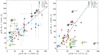 |
Fig. 5. Scatter plots of average pEW values for the SE SNe in our sample. He I λ7065 vs. He I λ5876 calculated between +10 d and +20 d, along with the best-fit relation pEWλ5876 = 30 + 1.3 × pEWλ7065 as a dashed line (left panel). O I λ7774 vs. He I λ7065 at +25 d to +45 d with the best-fit relation pEWλ7065 = 1.0 × pEWλ7774 (right panel). An illustrative set of SNe have been labeled by their abbreviated (i)PTF names in both panels. Yellow diamonds indicate all objects showing very broad LCs. |
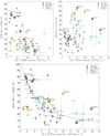 |
Fig. 6. Average pEW vs. velocity of He I λ7065 between +10 and +20 d (top-left panel). Average pEW vs. velocity of O I λ7774 between +10 and +20 d (top-right panel). Average pEW of He I λ7065 vs. velocity of O I λ7774 between +10 d and +20 d for SNe IIb and Ib, and the pEW of O I λ7774 scaled down by a factor of 2.2 vs. O I λ7774 velocity for SNe Ic (bottom panel). An illustrative set of SNe have been labeled by their abbreviated (i)PTF names. Yellow diamonds indicate all objects showing very broad LCs. In the bottom panel the thick dashed black line indicates the best-fit relation pEW∝ υ−2. The dashed vertical lines indicate the velocity increase expected from the Arnett (1982) model by removing 0.2 M⊙of material from the ejecta (the He envelope) for each line from left to right (mass-difference labels follow the thick dashed black line). The model has been scaled, so that the O I λ7774 velocity predicted for a total ejecta mass of 2.1 M⊙ is 4900 km s−1, to match the observed velocities of SN 2011dh (PTF11eon) and PTF12os. Two SNe IIb (iPTF15cna and PTF10qrl) are strong outliers from the fitted trend. These two SNe have very broad LCs and low O I λ7774 velocities (see Sect. 6 for further discussion). |
5.1. The helium shell
We find that there is a correlation between the pEWs of He I λ7065 and He I λ5876 (top-left panel of Fig. 5; measured by computing the average pEW between +10 d and +20 d for each SN). There is a large scatter, but the trend appears to be the same for both SNe IIb and Ib, and we get r = 0.66 and p < 0.001, when combining the values of SNe IIb and Ib. There is no statistically significant correlation for SNe Ic (r = 0.48, p < 0.12). This supports an interpretation where both of these lines are dominated by He in SNe IIb and Ib but not in SNe Ic. The latter is also indicated by the difficulty in obtaining a velocity estimate for He I λ5876 for SNe Ic (Sect. 4.2.1).
For Type Ic SNe there is a large spread in the pEWs of He I λ5876, but not in He I λ7065. This could indicate that Na I contamination is quite significant and might be causing most of the scatter (see, e.g., Dessart et al. 2015). A linear fit that excludes SNe Ic gives the relation pEWλ5876 = 30(±17) + 1.3(±0.3) × pEWλ7065 [Å], consistent with a 1:1 relation. Furthermore, we find that the trend is similar when calculated for any time interval of similar duration between −10 d and +50 d.
In the top-left panel of Fig. 6 we show the average velocity vs. the average pEW of the He I λ7065 absorption line measured between +10 d and +20 d. For SNe IIb and Ib there is a decreasing trend, with higher velocities giving weaker absorptions (r = −0.63, p < 0.001). This is what would be expected for He shells of lower mass being accelerated to higher velocities, assuming similar kinetic energies in the SN explosions. We find a similar trend for the He I λ5876 line during the same time interval (not shown). The trend in He I λ7065 is statistically significant when the averages are calculated for all intervals starting from −10 d and ending at +40 d. Prior to −10 d, the signatures from He I λ7065 are generally very weak (see Fig. 2).
5.2. The oxygen shell
To probe the oxygen-absorbing region of the ejecta, we compare the average pEW calculated between +25 d and +45 d for O I λ7774 vs. He I λ7065 (right panel of Fig. 5). For both SNe IIb and Ib there is an increasing trend with objects showing stronger O I λ7774 features also having stronger He I λ7065 (r = 0.73, p < 0.001 when SNe IIb and Ib are combined). A linear fit, excluding SNe Ic, gives a relation consistent with pEWλ7065 = 1.0 × pEWλ7774. For the SNe Ic in Fig. 5, we find no statistically significant correlation between the pEWs.
The pEW of He I λ7065 is always low, but it can be associated with a wide range of pEWs of O I λ7774. For time intervals earlier than +20 d, the trend for SNe IIb and Ib disappears, and around peak brightness the pEWs appear to be randomly scattered.
In the top-right panel of Fig. 6 we show the average velocity against the average pEW of the O I λ7774 absorption line measured between +10 d and +20 d. SNe IIb and Ib are scattered with no apparent correlations at lower absorptions and velocities compared to the SNe Ic in our sample (although there are a few outliers among all three subtypes). For SNe Ic there is a decreasing trend, with higher velocities corresponding to weaker absorptions (r = −0.50, p < 0.024). Similarly as what we found for the He shell, this could indicate that we are observing O shells of lower mass being accelerated to higher velocities. The lack of such a trend for SNe Ib and IIb would be expected, since the O absorbing region is located rather deep inside the ejecta behind significant amounts of He during this phase.
In the bottom panel of Fig. 6 we show the average velocity of the O I λ7774 absorption line vs. the average pEW of the He I λ7065 absorption line, measured between −10 d and +10 d for SNe IIb, Ib, and Ib/c; for SNe Ic, the average pEW/2.2 of O I λ7774 vs. O I λ7774 velocity is shown. SNe IIb and Ib that exhibit fast O (>8000 km s−1) also show weak He absorption (r = −0.65, p < 0.001). To show weak He absorption, we must have faster He (the top-left panel of Fig. 6). These findings, taken together, suggest that to see strong and fast O (i.e., the SNe Ic in our sample), the He envelope must have been physically removed. The trend seen for SNe IIb and Ib is consistent with the trend in pEW vs. velocity of O I λ7774 in SNe Ic, if the pEW is scaled down by a factor of 2.2. This suggests that the stripping does not necessarily stop as the He envelope is lost; some SNe Ic could be experiencing significant stripping of material from their C–O cores. Higher kinetic energy could also explain the higher velocities in SNe Ic, but it is difficult to explain why this would simultaneously lead to lower pEWs (see Sect. 6 for further discussion).
6. Discussion and future outlook
The pEWs and velocities we have measured are generally consistent with those previously reported by Matheson et al. (2001), Liu et al. (2016), and Prentice & Mazzali (2017)9. SNe Ic are faster and show stronger O pEWs in early-time spectra compared to the other SE SN subtypes, He pEW is anticorrelated with He and O velocities for SNe IIb and Ib, and O pEW appears anticorrelated with O velocity for SNe Ic. LC sample studies show no robust evidence for larger average ejecta masses or explosion energies in SNe Ic, compared to SNe IIb and Ib, that could result in faster and stronger oxygen signatures. Therefore, we agree with Matheson et al. (2001) and Liu et al. (2016); in order to have fast and strong O absorption at early times in most SNe Ic, the simplest explanation would be that we are immediately seeing into their C–O cores; their H and He envelopes have been physically removed prior to the explosions due to stellar winds or binary mass transfer.
However, models by Dessart et al. (2012) suggest that differences in 56Ni mixing could give rise to both SNe Ic and Ib, from similar progenitors with significant He envelopes (∼1.5 M⊙). In these models SNe Ic have low mixing, so that the radioactive 56Ni is never close enough to nonthermally excite the He in the envelope. Conversely, SNe Ib must have highly mixed 56Ni, in order to display observable He lines. A consequence of the lower mixing in these models is narrower and weaker absorption lines, along with lower velocities measured from absorption minima (especially for the O I λ7774 absorption; see Fig. 13 in Dessart et al. 2012). Thus, the results by Dessart et al. (2012) can be interpreted such that, if different 56Ni mixing is the main difference between the SE SN subtypes, SNe Ic should on average show both slower and weaker O I λ7774 absorption.
Our results are not consistent with such low mixing models; for the SNe Ic in our sample we find on average both stronger O I λ7774 absorption (Fig. 3) and faster velocities (Fig. 4) at early times. Liu et al. (2016) used a comparable result to argue against low-mixing models for SNe Ic, with the supporting evidence that LC studies show that SNe Ib and Ic seem to have progenitors of similar mass10. However, if SNe Ic came from higher energy explosions and significantly more massive progenitors compared to SNe Ib, the result could be higher kinetic energies in the C–O layer, consistent with stronger and faster O signatures. Furthermore, if the 56Ni is not significantly mixed into the outer He envelopes, there will be no He signatures, and models for the bolometric LC will underestimate the total ejecta masses (and the derived progenitor masses for SNe Ic), since the outer parts of the envelope devoid of 56Ni would not contribute to the LC (Piro & Morozova 2014). Anderson et al. (2012) suggested that SNe Ic prefer younger stellar populations, which could be consistent with larger progenitor masses (>30 M⊙). LC studies also suggest that the most massive SE SNe could have higher explosion energies (e.g., Lyman et al. 2016). Thus, low-mixing models for SNe Ic cannot easily be ruled out based on just a comparison of average O strengths and velocities among the subtypes.
To address this issue we looked for correlations among the quantities we have measured (Sect. 5). In particular, we found that there is an anticorrelation between He pEW and O velocity for SNe Ib and IIb, as well as between O pEW and velocity in SNe Ic (bottom panel, Fig. 6). To explain this behavior with models with gradually increasing kinetic energy (progenitor mass), and 56Ni mixed in such a way that the He gradually disappears, would require a significant amount of finetuning. The nickel mixing would have to decrease drastically as the kinetic energy increases, which seems counterintuitive since higher velocity ejecta imply higher velocity 56Ni. The alternative to this complicated scenario would be that the He envelope is gradually stripped off – a much more elegant solution. Thus, we conclude that He most likely is not hidden in SNe Ic due to low mixing11. Furthermore, early LC studies of SE SNe indicate that the 56Ni mixing appears to be high among all SE SN subtypes (Taddia et al. 2015), and possibly the highest for SNe Ic. Thus, models for normal SNe Ic should have high mixing, similar to the level of mixing needed for good spectral matches to SNe Ib.
If He cannot be hidden in typical SE SNe due to mixing, the anticorrelation between He pEW and O/He velocities in Fig. 6 suggests that envelopes with a wide range of He masses or abundances can be present at the time of explosion, since there appears to be a continuum from SNe Ib to Ic in this phase space (top-left panel, Fig. 6). This could be due to progenitors from a range of initial masses undergoing a similar amount of stripping, or a continuum in the amount of stripping experienced by the progenitor stars, or a combination thereof12. Furthermore, if higher mixing or kinetic energies were the cause of the increasing O I λ7774 velocities from SNe Ib to Ic, there is no clear explanation why the He lines would disappear as the mixing or kinetic energy increases. For very high velocities (≳20 000 km s−1), spectra do become gradually more featureless (like SNe Ic-BL), and it would be difficult to measure pEWs following our prescription (Sect. 3.3); but we are here dealing with much lower velocities (≲10 000 km s−1). From the models by Dessart et al. (2016), it is also clear that varying the kinetic energy, within typical ranges for SE SNe, will not change the observed SN type from a SN Ib to a SN Ic.
In particular, we find that the relation for the pEW of He I λ7065 and the O I λ7774 velocity in SNe IIb and Ib can be fit by pEW∝ υ−2 (Fig. 6). This suggests that there could be a simple relation between absorption strength and the mass of the He envelope in SE SNe, since  (Arnett 1982). If we assume that Ek remains unchanged as the velocity increases, and scale this relation so that the O I λ7774 velocity predicted for a total ejecta mass of 2.1 M⊙ is 4900 km s−1 to match the observed velocities and masses of SN 2011dh (PTF11eon) and PTF12os (Fremling et al. 2016), we find that to turn these SNe IIb into SNe Ic13, roughly 1.0–1.6 M⊙ of He would have to be removed (see the dashed vertical lines in the bottom panel of Fig. 6). This is consistent with the He envelope mass used in spectral models of SN 2011dh (e.g., Jerkstrand et al. 2015). Modeling work also clearly shows that a range of He envelope masses produces He signatures of various strengths (see, e.g., Fig. 11 in Hachinger et al. 2012). However, the exact relationship between He absorption pEW and He envelope mass has not been investigated. We strongly encourage future modeling efforts in this direction. Since the anticorrelation between He pEW and O velocity for SNe IIb and Ib is consistent with the behavior of O pEW and velocity in SNe Ic, our data also support the idea that some SE SNe can experience significant stripping all the way into their C–O cores14.
Dessart et al. (2016) have suggested that the best way to constrain the explosion parameters (e.g., total kinetic energy and ejecta mass) for SE SNe is to use the expansion rate of the ejecta ( ) derived from the He I λ5876 absorption line for SNe IIb and Ib and from the O I λ7774 line for SNe Ic, instead of υph in the Arnett (1982) model. If we assume that the average kinetic energy among the SN Ib and Ic subtypes is the same, we can use the observed He I and O I velocities for SNe Ib and Ic at maximum light (see Table 1 and the middle-right panel of Fig. 4) to roughly estimate what mass difference these velocities would imply for these subclasses, which could be interpreted as the average mass of the He envelope that is lost in a SN Ic. Using the relation between the ejecta mass (Mej) and the kinetic energy (Ek) for a constant density sphere expanding homologously (e.g., Lyman et al. 2016),
 (2)
(2)
we find with15 Vm−Ib = (9500 − 2640)/0.765 ≈ 9000 km s−1, Vm−Ic = (9800−2990)/0.443 ≈ 15 000 km s−1, Ek = 1×1051 erg, and Mej−Ib = 2.1 M⊙, that the Vm difference can be reproduced by removing 1.4 M⊙ of material from the envelope for an average SN Ib (note the similarity to the result based on the O velocity for SN 2011dh above). However, these calculations hold only if Ek really is the same (on average) between the subtypes. This is not necessarily the case; binary models of SE SNe typically require slightly higher initial masses to produce SNe Ic compared to SNe Ib (Yoon 2015). Thus, SNe Ic could have slightly larger C–O cores, and higher kinetic energies, so that the final ejecta masses derived from bolometric LC fitting end up very close to those of SNe Ib. This could affect our estimate of the average He mass that is lost in a SN Ic, but the anticorrelations we have found between pEW and velocity for both He and O cannot easily be explained without removing mass from the envelopes. Spectral modeling efforts in combination with hydrodynamical modeling are needed in order to make more quantitative statements.
Piro & Morozova (2014) suggested that SN 2011dh and iPTF13bvn could have a significant amount of transparent He, based on their low He absorption velocities (which would result in underestimated ejecta masses derived from their LCs). We do find low velocities in these SNe. However, at the same time, they show some of the strongest He I λλ5876, 7065 absorption features in our sample (see, e.g., the bottom panel of Fig. 6). This would not be expected if only a small inner part of the He envelope is producing the observed He lines. In the top-left panel of Fig. 6 there are only two SNe IIb at velocities lower than ∼7000 km s−1 that also show low pEWs. Thus, while this effect could be present in a few objects, it does not appear to be dominating. We also found that SNe Ib and IIb show a trend with high He pEW values correlated to low velocities (see Fig. 6). This is also inconsistent with partly transparent He envelopes being typical for these subtypes; we would expect to have more objects at both low pEW and low velocity (only a small part of the He envelope is emitting, and it should be slow since the emitting region would be located behind an outer transparent envelope of significant mass).
There are two SNe IIb (PTF10qrl and iPTF15cna) in our sample that show weak He I λ7065 absorption, along with very low O I λ7774 velocities (bottom panel of Fig. 6). At the same time, their LCs are very broad (stretched by a factor of ∼2, compared to SN 2011dh; Karamehmetoglu et al., in prep.). This indicates that they likely come from massive progenitor stars (≳30 M⊙). For such progenitors, even models with high mixing can have difficulties in producing He signatures, since the He envelope is far from the center of the explosion outside a large C–O core (Dessart et al. 2015; Dessart et al. 2016). In these models there is some transparent helium, leading to weak or no He signatures, along with low expansion velocities of O I λ7774 (since the O is slowed down by a significant He envelope), consistent with our observations of these two SNe. These objects can also be used as an argument against the suggestion by Frey et al. (2013) that very massive stars (≳23 M⊙) would all become SNe Ic with enhanced O abundances in their outer envelopes owing to strong stellar mixing. The top-right panel of Fig. 6 shows that the majority of SE SNe with broad LCs do not exhibit significantly enhanced O absorption.
Going forward, we are in the process of modeling the bolometric LCs of all SE SNe found by (i)PTF, using expansion velocities derived from the He I λ5876 line for SNe IIb and Ib and from the O I λ7774 line for SNe Ic. A data-release paper for the full (i)PTF SE SN spectral sample is also in progress, which will supplement the analysis presented here (Fremling et al., in prep.).
7. Conclusions
The main conclusions of this work are as follows.
SNe Ic show higher O I pEWs and O I velocities compared to SNe IIb and Ib (higher by ∼50 Å and ∼2000 km s−1, at maximum light). This is inconsistent with what would be expected if low mixing was responsible for hiding He signatures in SNe Ic. SNe Ic likely lack He shells; removing the He shell will give higher velocities in the O shell for the same kinetic energy in the explosion.
The He I λλ5876, 7065 velocities at maximum light are higher in SNe Ib compared to SNe IIb. (∼1000 km s−1 higher). The lack of an outer H shell in SNe Ib allow higher velocities to be reached in the He shell as the SN shock wave passes through the ejecta.
The pEWs of the He I λλ5876, 7065 absorption lines are similar past maximum light in most SNe Ib and SNe IIb. The He shells appear to be very similar among SNe IIb and Ib.
There is an anticorrelation between He I λ7065 pEW and O I λ7774 velocity among SNe IIb and Ib. This can be interpreted as a difference in the amount of He at the time of explosion. The observed difference in the expansion rate of the ejecta around maximum light for SNe Ic and Ib imply an average He mass difference of 1.4 M⊙, if all other explosion parameters are assumed to be unchanged between SNe Ic and Ib. The difference could either be on account of different starting progenitor masses that undergo a similar amount of stripping, or a continuum in the extent of stripping of the He envelope from progenitors of similar initial mass, or a combination thereof.
Only two objects in the entire sample (PTF10qrl and iPTF15cna) show both low pEWs of He and slow velocities of either He or O. Both of these objects have very broad LCs, atypical for SE SNe. Therefore, we find that our sample does not show compelling evidence for hidden He in normal SE SNe.
When discussing this line we effectively refer to the O I λλ7771, 7774, 7775 triplet.
Approximately 20.5 and 21 mag in the Mould R and Sloan ℊ bands, respectively.
This is potentially important since (i)PTF could find SE SNe in hosts with very low metallicity compared to the average for SE SNe (e.g., Sanders et al. 2012). Two examples are iPTF15dtg (Taddia et al. 2016) and PTF11mnb (Taddia et al. 2018). However, their spectra are similar to those of normal SNe Ic, and we do not find any significant differences in our results compared to Matheson et al. (2001) and Liu et al. (2016). Thus, a detailed analysis of the impact of (i)PTF being untargeted was not performed.
By comparing observed spectra to the models by Dessart et al. (2012), as was previously done by Liu et al. (2016).
See Ergon et al. (2014, 2015), for a detailed investigation of SN 2011dh.
For spectra of very low S/N we get uncertainties on the order of 25 Å in our peak position estimates.
We use polynomials of degree 4–7 depending on the feature shape and quality of the spectrum.
This study was based largely on the same sample as Liu et al. (2016), and the results are consistent between the two papers for the He line strengths and velocities. The O lines were not analyzed by Prentice & Mazzali (2017).
With progenitors of similar mass, the stronger O signatures in SNe Ic would be explained by a lack of a He envelope.
See also Hachinger et al. (2012), who have shown that more than ∼0.1 M⊙ of He cannot be hidden in highly mixed SE SN models.
Since the transition in He pEW from SNe Ib to SNe Ic is continuous, there is a range where making the distinction between these subtypes can be ambiguous and dependent on the quality of the spectra (see Liu et al. 2016; Shivvers et al. 2017, for further discussion).
In terms of reaching typical SN Ic O I λ7774 velocities between +10 d and +20 d, which are 6000–10 000 km s−1, for 66.7% of the SN Ic population.
See, e.g., SN 2005ek, possibly the result of mass transfer from a He star to a compact companion in a very close binary (Drout et al. 2013; Tauris et al. 2013).
Vm relations from Dessart et al. (2016).
Acknowledgments
We gratefully acknowledge support from the Knut and Alice Wallenberg Foundation. The Oskar Klein Centre is funded by the Swedish Research Council. We acknowledge the contributions from the full PTF and iPTF collaborations that made it possible to discover and monitor the SE SNe analyzed in this work. This work was supported by the GROWTH project funded by the National Science Foundation (NSF) under grant AST-1545949. D.A.H. and G.H. are supported by NSF grant AST-1313484. A.V.F. is grateful for financial assistance from NSF grant AST-1211916, the TABASGO Foundation, the Christopher R. Redlich Fund, and the Miller Institute for Basic Research in Science (UC Berkeley). His work was conducted in part at the Aspen Center for Physics, which is supported by NSF grant PHY-1607611; he thanks the Center for its hospitality during the neutron stars workshop in June and July 2017. Research at Lick Observatory is partially supported by a generous gift from Google. Some of the data presented herein were obtained at the W. M. Keck Observatory, which is operated as a scientific partnership among the California Institute of Technology, the University of California, and NASA; the observatory was made possible by the generous financial support of the W. M. Keck Foundation. This work is based in part on observations from the LCO network. The William Herschel Telescope is operated on the island of La Palma by the Isaac Newton Group of Telescopes in the Spanish Observatorio del Roque de los Muchachos of the Instituto de Astrofísica de Canarias, which is also the site of the Nordic Optical Telescope (NOT) and the Gran Telescopio Canarias (GTC). This work is partly based on observations made with DOLoResatTNG. Our results made use of the Discovery Channel Telescope (DCT) at Lowell Observatory. Lowell is a private, nonprofit institution dedicated to astrophysical research and public appreciation of astronomy, and it operates the DCT in partnership with Boston University, the University of Maryland, the University of Toledo, Northern Arizona University, and Yale University. The upgrade of the DeVeny optical spectrograph has been funded by a generous grant from John and Ginger Giovale. Initial classification of some SNe was done with the SuperNova Integral Field Spectrograph (SNIFS) on the University of Hawaii 2.2 m telescope as part of the Nearby Supernova Factory II project. We acknowledge the large number of observers and reducers that helped aquire this spectroscopic database over the years, including R. Ellis and M. Sullivan for contributing spectral data obtained under their respective observing programs. A.V.F. thanks the following members of his group for assistance with the observations and reductions: J. Choi, R. J. Foley, O. D. Fox, M. Kandrashoff, P. J. Kelly, I. Kleiser, J. Kong, A. Miller, A. Morton, D. Poznanski, and I. Shivvers. We thank the staffs at the observatories where data were obtained.
References
- Anderson, J. P., Habergham, S. M., James, P. A., & Hamuy, M. 2012, MNRAS, 424, 1372 [NASA ADS] [CrossRef] [Google Scholar]
- Appenzeller, I., Fricke, K., Fürtig, W., et al. 1998, The Messenger, 94, 1 [NASA ADS] [Google Scholar]
- Arcavi, I., Gal-Yam, A., Yaron, O., et al. 2011, ApJ, 742, L18 [NASA ADS] [CrossRef] [Google Scholar]
- Arnett, W. D. 1982, ApJ, 253, 785 [NASA ADS] [CrossRef] [Google Scholar]
- Ben-Ami, S., Gal-Yam, A., Filippenko, A. V., et al. 2012, ApJ, 760, L33 [NASA ADS] [CrossRef] [Google Scholar]
- Ben-Ami, S., Gal-Yam, A., Mazzali, P. A., et al. 2014, ApJ, 785, 37 [NASA ADS] [CrossRef] [Google Scholar]
- Benn, C., Dee, K., & Agócs, T. 2008, in Ground-based and Airborne Instrumentation for Astronomy II, Proc. SPIE, 7014, 70146X [CrossRef] [Google Scholar]
- Blondin, S., & Tonry, J. L. 2007, ApJ, 666, 1024 [NASA ADS] [CrossRef] [Google Scholar]
- Cano, Z. 2013, MNRAS, 434, 1098 [NASA ADS] [CrossRef] [Google Scholar]
- Cao, Y., Nugent, P. E., & Kasliwal, M. M. 2016, PASP, 128, 114502 [NASA ADS] [CrossRef] [Google Scholar]
- Claeys, J. S. W., de Mink, S. E., Pols, O. R., Eldridge, J. J., & Baes, M. 2011, A&A, 528, A131 [NASA ADS] [CrossRef] [EDP Sciences] [Google Scholar]
- Conti, P. 1976, MSRSL, 9, 193 [Google Scholar]
- Dessart, L., & Hillier, D. J. 2005, A&A, 439, 671 [NASA ADS] [CrossRef] [EDP Sciences] [Google Scholar]
- Dessart, L., Hillier, D. J., Li, C., & Woosley, S. 2012, MNRAS, 424, 2139 [NASA ADS] [CrossRef] [Google Scholar]
- Dessart, L., Hillier, D. J., Woosley, S., et al. 2015, MNRAS, 453, 2189 [NASA ADS] [CrossRef] [Google Scholar]
- Dessart, L., Hillier, D. J., Woosley, S., et al. 2016, MNRAS, 458, 1618 [NASA ADS] [CrossRef] [Google Scholar]
- Dressler, A., Bigelow, B., Hare, T., et al. 2011, PASP, 123, 288 [NASA ADS] [CrossRef] [Google Scholar]
- Drout, M. R., Soderberg, A. M., Gal-Yam, A., et al. 2011, ApJ, 741, 97 [NASA ADS] [CrossRef] [Google Scholar]
- Drout, M. R., Soderberg, A. M., Mazzali, P. A., et al. 2013, ApJ, 774, 58 [NASA ADS] [CrossRef] [Google Scholar]
- Ergon, M., Sollerman, J., Fraser, M., et al. 2014, A&A, 562, A17 [NASA ADS] [CrossRef] [EDP Sciences] [Google Scholar]
- Ergon, M., Jerkstrand, A., Sollerman, J., et al. 2015, A&A, 580, A142 [NASA ADS] [CrossRef] [EDP Sciences] [Google Scholar]
- Faber, S. M., Phillips, A. C., Kibrick, R. I., et al. 2003, in Instrument Design and Performance for Optical/Infrared Ground-based Telescopes, eds. M. Iye, & A. F. M. Moorwood, Proc. SPIE, 4841, 1657 [NASA ADS] [CrossRef] [Google Scholar]
- Filippenko, A. V. 1997, ARA&A, 35, 309 [NASA ADS] [CrossRef] [Google Scholar]
- Folatelli, G., Bersten, M. C., Kuncarayakti, H., et al. 2014, ApJ, 792, 7 [NASA ADS] [CrossRef] [Google Scholar]
- Fremling, C., Sollerman, J., Taddia, F., et al. 2014, A&A, 565, A114 [NASA ADS] [CrossRef] [EDP Sciences] [Google Scholar]
- Fremling, C., Sollerman, J., Taddia, F., Ergon, M., & Fraser, M. 2016, A&A, 593, A68 [NASA ADS] [CrossRef] [EDP Sciences] [Google Scholar]
- Frey, L. H., Fryer, C. L., & Young, P. A. 2013, ApJ, 773, L7 [NASA ADS] [CrossRef] [Google Scholar]
- Gal-Yam, A. 2016, ArXiv e-prints [arXiv:1611.09353] [Google Scholar]
- Gal-Yam, A., Arcavi, I., Ofek, E. O., et al. 2014, Nature, 509, 471 [NASA ADS] [CrossRef] [Google Scholar]
- Guillochon, J., Parrent, J., Kelley, L. Z., & Margutti, R. 2017, ApJ, 835, 64 [NASA ADS] [CrossRef] [Google Scholar]
- Hachinger, S., Mazzali, P. A., Taubenberger, S., et al. 2012, MNRAS, 422, 70 [NASA ADS] [CrossRef] [Google Scholar]
- Hill, G. J., Nicklas, H. E., MacQueen, P. J., et al. 1998, in Optical Astronomical Instrumentation, ed. S. D’Odorico, Proc. SPIE, 3355, 375 [NASA ADS] [CrossRef] [Google Scholar]
- Hook, I. M., Jørgensen, I., Allington-Smith, J. R., et al. 2004, PASP, 116, 425 [NASA ADS] [CrossRef] [Google Scholar]
- Horesh, A., Kulkarni, S. R., Corsi, A., et al. 2013, ApJ, 778, 63 [NASA ADS] [CrossRef] [Google Scholar]
- Iben, Jr., I., & Tutukov, A. V. 1985, ApJS, 58, 661 [NASA ADS] [CrossRef] [Google Scholar]
- Jerkstrand, A., Ergon, M., Smartt, S. J., et al. 2015, A&A, 573, A12 [NASA ADS] [CrossRef] [EDP Sciences] [Google Scholar]
- Kasliwal, M. M., Kulkarni, S. R., Gal-Yam, A., et al. 2010, ApJ, 723, L98 [NASA ADS] [CrossRef] [Google Scholar]
- Lantz, B., Aldering, G., Antilogus, P., et al. 2004, in Optical Design and Engineering, eds. L. Mazuray, P. J. Rogers, & R. Wartmann, Proc. SPIE, 5249, 146 [NASA ADS] [CrossRef] [Google Scholar]
- Law, N. M., Kulkarni, S. R., Dekany, R. G., et al. 2009, PASP, 121, 1395 [NASA ADS] [CrossRef] [Google Scholar]
- Liu, Y., & Modjaz, M. 2014, ArXiv e-prints [arXiv:1405.1437] [Google Scholar]
- Liu, Y.-Q., Modjaz, M., Bianco, F. B., & Graur, O. 2016, ApJ, 827, 90 [NASA ADS] [CrossRef] [Google Scholar]
- Lyman, J. D., Bersier, D., James, P. A., et al. 2016, MNRAS, 457, 328 [NASA ADS] [CrossRef] [Google Scholar]
- Masci, F. J., Laher, R. R., Rebbapragada, U. D., et al. 2017, PASP, 129, 014002 [NASA ADS] [CrossRef] [Google Scholar]
- Matheson, T., Filippenko, A. V., Li, W., Leonard, D. C., & Shields, J. C. 2001, AJ, 121, 1648 [NASA ADS] [CrossRef] [Google Scholar]
- Modjaz, M., Blondin, S., Kirshner, R. P., et al. 2014, AJ, 147, 99 [NASA ADS] [CrossRef] [Google Scholar]
- Nordin, J., Östman, L., Goobar, A., et al. 2011, A&A, 526, A119 [NASA ADS] [CrossRef] [EDP Sciences] [Google Scholar]
- Oke, J. B., & Gunn, J. E. 1982, PASP, 94, 586 [NASA ADS] [CrossRef] [Google Scholar]
- Oke, J. B., Cohen, J. G., Carr, M., et al. 1995, PASP, 107, 375 [NASA ADS] [CrossRef] [Google Scholar]
- Osip, D. J., Floyd, D., & Covarrubias, R. 2008, in Ground-based and Airborne Instrumentation for Astronomy II, Proc. SPIE, 7014, 70140A [CrossRef] [Google Scholar]
- Piro, A. L., & Morozova, V. S. 2014, ApJ, 792, L11 [NASA ADS] [CrossRef] [Google Scholar]
- Prentice, S. J., & Mazzali, P. A. 2017, MNRAS, 469, 2672 [NASA ADS] [CrossRef] [Google Scholar]
- Prentice, S. J., Mazzali, P. A., Pian, E., et al. 2016, MNRAS, 458, 2973 [NASA ADS] [CrossRef] [Google Scholar]
- Sanders, N. E., Soderberg, A. M., Levesque, E. M., et al. 2012, ApJ, 758, 132 [NASA ADS] [CrossRef] [Google Scholar]
- Shivvers, I., Modjaz, M., Zheng, W., et al. 2017, PASP, 129, 054201 [NASA ADS] [CrossRef] [Google Scholar]
- Smith, N. 2014, ARA&A, 52, 487 [NASA ADS] [CrossRef] [MathSciNet] [Google Scholar]
- Strotjohann, N. L., Ofek, E. O., Gal-Yam, A., et al. 2015, ApJ, 811, 117 [NASA ADS] [CrossRef] [Google Scholar]
- Sun, F., & Gal-Yam, A. 2017, ArXiv e-prints [arXiv:1707.02543] [Google Scholar]
- Taddia, F., Sollerman, J., Leloudas, G., et al. 2015, A&A, 574, A60 [NASA ADS] [CrossRef] [EDP Sciences] [Google Scholar]
- Taddia, F., Fremling, C., Sollerman, J., et al. 2016, A&A, 592, A89 [NASA ADS] [CrossRef] [EDP Sciences] [Google Scholar]
- Taddia, F., Sollerman, J., Fremling, C., et al. 2018, A&A, 609, A106 [NASA ADS] [CrossRef] [EDP Sciences] [Google Scholar]
- Tauris, T. M., Langer, N., Moriya, T. J., et al. 2013, ApJ, 778, L23 [NASA ADS] [CrossRef] [Google Scholar]
- Yaron, O., & Gal-Yam, A. 2012, PASP, 124, 668 [NASA ADS] [CrossRef] [Google Scholar]
- Yoon, S.-C. 2015, PASA, 32, 15 [NASA ADS] [CrossRef] [Google Scholar]
- Yoon, S.-C., Woosley, S. E., & Langer, N. 2010, ApJ, 725, 940 [NASA ADS] [CrossRef] [Google Scholar]
Appendix A: Additional table
Spectral log for the (i)PTF SE SN sample.
All Tables
All Figures
|
Fig. 1. Description of our pEW and expansion-velocity measurement method using spectra around peak brightness for iPTF13bvn (Type Ib, +0.5 d, upper blue line), SN 2011dh (Type IIb, +2.5 d, middle red line), and PTF10osn (Type Ic, +4.0 d, bottom green line). On the spectrum of SN 2011dh, the absorption features of He I λλ5876, 7065 and O I λ7774 have been labeled with numbers. Measurements of features 1–3 have been attempted on all spectra in our sample. For SE SNe, feature 1 is typically associated with He I λ5876, feature 2 with He I λ7065, and feature 3 with O I λ7774, although other elements also contribute to these features. Dashed red lines indicate pseudo-continuum estimates (first-order polynomial fits) for features 1–3 resulting from our measurement scheme (Sect. 3). We calculate pEWs (e.g., Fig. 2) between the endpoints of these continuum estimates using Eq. (1). Velocity estimates are obtained by locating the minima of polynomial fits between the pseudo-continuum endpoints (order 4–7, dashed black lines). If a spectral feature is ambiguous, and has several minima within a similar range as shown for feature 2 in the spectrum of PTF10osn, we set the velocity estimate to be undefined but still calculate the pEW. Wavelengths have been shifted to the rest frame, and the spectra have been normalized and shifted by a constant for clarity. |
| In the text | |
|
Fig. 2. Absorption strengths of He I λ5876 (left panels) and He I λ7065 (right panels). Top panels: individual measurements, with multiple measurements of the same SN connected by solid lines. Middle panels: averages of the SE SN subtypes, with error bars representing the standard deviation of the mean. Dashed lines outline the standard deviations of the samples for each subtype in matching color. Bottom panels: CDFs measured between −10 and +10 d |
| In the text | |
|
Fig. 3. Absorption strengths of O I λ7774. Top panel: individual measurements, with multiple measurements of the same SN connected by solid lines. Middle panel: the averages of the SE SN subtypes, with error bars representing the standard deviation of the mean. Dashed lines outline the standard deviations of the samples for each subtype in matching color. Bottom panel: CDFs measured between −10 and +10 d. |
| In the text | |
|
Fig. 4. Velocities of He I λ5876 (left panels) and O I λ7774 (right panels). Top panels: individual measurements, with measurements of the same SN connected by solid lines. Middle panels: averages of the SE subtypes, with error bars representing the standard deviation of the mean. Dashed lines outline the standard deviations of the samples for each subtype in matching color. Average velocities derived from He I λ7065 are shown as thick solid lines (Type Ib in blue and Type IIb in red) in the middle-left panel. The average He I λ5876 velocity of Type Ib SNe is shown as a thick solid line in the middle-right panel. Bottom panels: CDFs measured between −10 and +10 d for each subtype. |
| In the text | |
|
Fig. 5. Scatter plots of average pEW values for the SE SNe in our sample. He I λ7065 vs. He I λ5876 calculated between +10 d and +20 d, along with the best-fit relation pEWλ5876 = 30 + 1.3 × pEWλ7065 as a dashed line (left panel). O I λ7774 vs. He I λ7065 at +25 d to +45 d with the best-fit relation pEWλ7065 = 1.0 × pEWλ7774 (right panel). An illustrative set of SNe have been labeled by their abbreviated (i)PTF names in both panels. Yellow diamonds indicate all objects showing very broad LCs. |
| In the text | |
|
Fig. 6. Average pEW vs. velocity of He I λ7065 between +10 and +20 d (top-left panel). Average pEW vs. velocity of O I λ7774 between +10 and +20 d (top-right panel). Average pEW of He I λ7065 vs. velocity of O I λ7774 between +10 d and +20 d for SNe IIb and Ib, and the pEW of O I λ7774 scaled down by a factor of 2.2 vs. O I λ7774 velocity for SNe Ic (bottom panel). An illustrative set of SNe have been labeled by their abbreviated (i)PTF names. Yellow diamonds indicate all objects showing very broad LCs. In the bottom panel the thick dashed black line indicates the best-fit relation pEW∝ υ−2. The dashed vertical lines indicate the velocity increase expected from the Arnett (1982) model by removing 0.2 M⊙of material from the ejecta (the He envelope) for each line from left to right (mass-difference labels follow the thick dashed black line). The model has been scaled, so that the O I λ7774 velocity predicted for a total ejecta mass of 2.1 M⊙ is 4900 km s−1, to match the observed velocities of SN 2011dh (PTF11eon) and PTF12os. Two SNe IIb (iPTF15cna and PTF10qrl) are strong outliers from the fitted trend. These two SNe have very broad LCs and low O I λ7774 velocities (see Sect. 6 for further discussion). |
| In the text | |
Current usage metrics show cumulative count of Article Views (full-text article views including HTML views, PDF and ePub downloads, according to the available data) and Abstracts Views on Vision4Press platform.
Data correspond to usage on the plateform after 2015. The current usage metrics is available 48-96 hours after online publication and is updated daily on week days.
Initial download of the metrics may take a while.