| Issue |
A&A
Volume 617, September 2018
|
|
|---|---|---|
| Article Number | A72 | |
| Number of page(s) | 24 | |
| Section | Planets and planetary systems | |
| DOI | https://doi.org/10.1051/0004-6361/201832780 | |
| Published online | 17 September 2018 | |
Color study of asteroid families within the MOVIS catalog
1
Instituto de Astrofísica de Canarias (IAC),
C/Vía Láctea s/n,
38205
La Laguna,
Tenerife,
Spain
e-mail: This email address is being protected from spambots. You need JavaScript enabled to view it.
2
Departamento de Astrofísica, Universidad de La Laguna,
38205
La Laguna,
Tenerife,
Spain
3
Astronomical Institute of the Romanian Academy,
5 Cuţitul de Argint,
040557
Bucharest,
Romania
Received:
6
February
2018
Accepted:
13
March
2018
Abstract
The aim of this work is to study the compositional diversity of asteroid families based on their near-infrared colors, using the data within the MOVIS catalog. As of 2017, this catalog presents data for 53 436 asteroids observed in at least two near-infrared filters (Y, J, H, or Ks). Among these asteroids, we find information for 6299 belonging to collisional families with both Y −J and J−Ks colors defined. The work presented here complements the data from SDSS and NEOWISE, and allows a detailed description of the overall composition of asteroid families. We derived a near-infrared parameter, the ML*, that allows us to distinguish between four generic compositions: two different primitive groups (P1 and P2), a rocky population, and basaltic asteroids. We conducted statistical tests comparing the families in the MOVIS catalog with the theoretical distributions derived from our ML* in order to classify them according to the above-mentioned groups. We also studied the background populations in order to check how similar they are to their associated families. Finally, we used this parameter in combination with NEOWISE and SDSS to check for possible bimodalities in the data. We found 43 families with ML*err < 0.071 and with at least 8 asteroids observed: 5 classified as P1, 10 classified as P2, 19 families associated with the rocky population, and 9 families that were not linked to any of the previous populations. In these cases, we compared our samples with different combinations of these theoretical distributions to find the one that best fits the family data. We also show, using the data from MOVIS and NEOWISE, that the Bapistina family presents a two-cluster distribution in the near-infrared albedo vs. ML* parameter space that might be related to a common differentiated parent body. Finally, we show that the backgrounds we defined seem to be linked to their associated families.
Key words: minor planets, asteroids: general / methods: data analysis / techniques: photometric
© ESO 2018
1 Introduction
Asteroid families are the remnants of catastrophic collisional episodes in the solar system. After such events, a large asteroid (commonly known as parent body) leaves behind dozens, hundreds, or even thousands of fragments that share similar orbital properties. These fragments, referred to as family members, experienced dynamical processes under the gravitational forces dominating the solar system and also via the Yarkovsky effect, gradually evolving to their current locations in the main asteroid belt (Bottke et al. 2002). By analyzing the physical properties of the family members, we can investigate the composition of the original bodies, and we can study the processes that these objects have experienced through the history of the solar system.
At the beginning of the 21st century, several all-sky surveys were carried out: SDSS (York et al. 2000) and Pan-STARRS (Kaiser et al. 2010) at optical wavelengths, and WISE (Wright et al. 2010), AKARI (Ishihara et al. 2010), and 2MASS (Skrutskie et al. 2006) at different infrared wavelengths. Initially, these surveys were mainly of cosmological or stellar interest. However, their sky coverage offers the opportunity to study a large number of solar system objects. Using data from some of these databases, combined with data from visible and infrared spectroscopic surveys, light curves, and polarimetry, Masiero et al. (2015) carried out an analysis of 109 out of the 122 families identified by Nesvorný et al. (2015). In their paper, they outlined some key questions that still remain unanswered, such as the effect of space weathering or the presence of inhomogeneities in asteroid family composition. Related to this last point, one of the most prominent questions is the apparent absence of collisional families generated from the complete disruption of a differentiated parent body.
In 2009, using the Visible and Infrared Survey Telescope for Astronomy (VISTA), several near-infrared surveys started to collect data in five broadband filters: Z, Y, J, H, and Ks (Sutherland et al. 2015). Among these, the VISTA Hemisphere Survey (VHS) aims to image almost the entire southern hemisphere, i.e., ~19 000−1 (McMahon et al. 2013). Using the third data release of this survey (VISTA VHS-DR3), Popescu et al. (2016) compiled their Moving Objects from VISTA Survey catalog (MOVIS), with a total of 39 947 solar system objects, including NEAs, main-belt asteroids, TNOs, comets, and other bodies. This catalog presents colors for those objects observed in at least two of the Y, J, H, and Ks infrared filters. See Fig. 1 for the response curves of these filters.
The work presented here aims to enhance the current knowledge about overall family composition and physical properties, and to complement the available information of the families with near-infrared photometry. To achieve this, we have used the latest version of the MOVIS database. This paper is organized as follows: we describe the latest version of the MOVIS catalog in Sect. 2, as well as the datasets used for family identification and data comparison; in Sect. 3 we define a near-infrared parameter that will be used to classify those families with a significant number of members observed within the catalog; in Sect. 4 we discuss the results for individual families; finally, in Sect. 5 we summarize the obtained results and we address some important questions to be investigated in the near future.
 |
Fig. 1 Response curves of the Y, J, H, and Ks VISTA filters (blue), together with the DeMeo et al. (2009) template spectra of the asteroid populations in our study. We averaged the templates for the B-, C-, and X-types and subclasses (primitives); the S-types and subclasses (rocky); and V-types (basaltic). The template spectra have been normalized to unity at 1.25 μm (central wavelength of the J filter) for representation purposes. |
2 Dataset description
To conduct our analysis we used several databases with physical data of thousands of asteroids. Here follows a brief description of each of these datasets.
2.1 Infrared colors from the MOVIS catalog
The main dataset that we use throughout this paper is the latest version of the Moving Objects from VISTA Survey (MOVIS) catalog1. It was compiled from data in the VISTA Hemisphere Survey (VHS), obtained using the VISTA telescope, a 4 m class telescope located at the ESO Cerro Paranal Observatory (Chile). Thanks to this survey, which aims to cover almost the whole sky of the southern hemisphere (McMahon et al. 2013), it was possible to retrieve spectro-photometric data in four near-infrared filters, Y, J, H, and Ks (see Fig. 1 and Table 1), and also accurate astrometry, for a very large number of solar system objects. A complete description of the creation of the MOVIS catalog can be found in Popescu et al. (2016). In particular, we use an updated version of the MOVIS-C catalog, compiled on April 30, 2017. This catalog was obtained using the VHSv20161007 data release of the VISTA Hemisphere Survey. It includes photometric colors (Y − J, Y − H, Y − Ks, J− H, J− Ks, and H− Ks) and errors for a total of 53 436 asteroids. Our analysis is performed using data in the Y, J, and Ks filters for a total of 18 263 objects. Figure 2 shows the distribution of these objects in proper orbital element space.
Central wavelengths and passbands for the different filters used in the SDSS (Bessell 2005), VISTA-VHSa, and NEOWISE (Jarrett et al. 2011) surveys.
2.2 Family lists
In order to look for family members within the objects present in the MOVIS catalog, we used the lists from Nesvorný et al. (2015). For the family identification process the authors took into account many past publications (Mothé-Diniz et al. 2005; Nesvorný et al. 2005; Gil-Hutton 2006; Parker et al. 2008; Nesvorny 2010, 2012; Novaković et al. 2011; Brož et al. 2013; Masiero et al. 2011, 2013; Carruba et al. 2013; Milani et al. 2014), as well as data from SDSS and NEOWISE, to finally define 122 asteroid families. These lists were created using numerically computed proper orbital elements for 384 337 numbered asteroids and 4016 Jupiter trojans. The dataset, publicly available in the Small Bodies Node of the NASA Planetary Data System2, provides thesynthetic proper orbital elements used to compute family membership, as well as values for the absolute magnitude of the asteroids (Hv). Some asteroids are included in more than one family; for example, all the members of the Beagle family are also included in the Themis family. In these cases we considered those asteroids as members of the smallest family (i.e., we removed the Beagle family members from the Themis family). We found 6299 asteroids belonging to 104 families among the MOVIS data and observed at least in the Y, J, and Ks filters (see Table A.1). These asteroids are shown in Fig. 2.
 |
Fig. 2 Proper semimajor axis vs. proper inclination (left panel) and proper eccentricity (right panel) for the asteroids observed within MOVIS catalog. The blue background represents the full sample of objects with Y − J and J− Ks colors defined in MOVIS (a total of 18 263 objects). In orange, we overplot those asteroids belonging to families (6299 objects). |
2.3 Other datasets: the SDSS MOC and NEOWISE
The Sloan Digital Sky Survey was initially devised to measure redshifts of large samples of galaxies (York et al. 2000; Ivezić et al. 2001). However, sky coverage and survey operations made it possible to observe a great number of asteroids in five photometric filters (u′, g′, r′, i′, z′) in optical wavelengths (see Table 1). The latest release of the Sloan Digital Sky Survey Moving Object Catalog (SDSS MOC) lists astrometric and photometric data for 471 569 moving objects observed up to March 2007. This catalog has been used to determine family membership (Ivezić et al. 2002), to constrain family size distribution (Parker et al. 2008), or even to perform photometric taxonomic classifications (Carvano et al. 2010; DeMeo & Carry 2013).
In a different wavelength range, the Near-Earth Object Wide-field Infrared Survey Explorer (NEOWISE, initially launched as WISE) performed an all-sky astronomical survey with images in four infrared photometric filters (see Table 1). This catalog contains data for over 150 000 asteroids (Mainzer et al. 2011, 2014). Using this dataset, Masiero et al. (2011) computed albedos and diameters for over 32 000 members of 46 collisional families from Nesvorny (2012), and from these diameters Masiero et al. (2013) measured the size-frequency distributions for 76 asteroid families identified within the data.
In this work we compare near-infrared albedos (pNIR) derived from the NEOWISE3 data, and the slope parameter a* derived from the SDSS4 observations, with the results obtained from our analysis of the MOVIS near-infrared colors (which covers the wavelength range between the SDSS and NEOWISE surveys) of the families present in the catalog.
3 Data processing
In order to differentiate between the asteroid populations in the MOVIS catalog, we define a single parameter (ML*) using the Y, J, and Ks spectro-photometric information. We followed a similar approach to that used in Ivezić et al. (2001) to derive the a*. We chose this parametrization because it favors the description of overall composition of asteroid groups. An in-depth taxonomic classification based on near-infrared colors and obtained with a machine-learning algorithm is presented in Popescu et al. (2018). This taxonomy favors the classification of individual asteroids into several classes and subclasses, and it is compatible with previous taxonomies, proposing targets for future spectral investigation.
3.1 The ML* parameter
We parametrized the photometry of the asteroids in the MOVIS database in order to determine how families are compatible with a “primitive” or “rocky” composition. This process followed four steps:
- 1.
We first removed the ten observed comets from the full MOVIS-C database. Then, taking into account our previous experience with data quality when creating the MOVIS catalog, we selected the subset of asteroids with computed colors Y −J and J−Ks having errors smaller than 0.15 magnitudes (C0.15). This yielded a total of 10 107 objects.
- 2.
We performed two bivariate kernel density estimations on this first selection with different resolutions using Python routines contained in the seaborn package (Waskom et al. 2017). Once we estimated the bivariate probability density functions (PDF), we extracted the values of the density maxima for the two main clusters present in the color–color plots, associated with S- and C-complex asteroids (Popescu et al. 2016).
- 3.
We then computed the angle between the line that connects the two maxima (determined in the previous step) and the x-axis of the system. Next, we rotated the system according to this angle, selecting the new y-axis as our parameter.
- 4.
We forced this parameter to be zero at the separation between the two main clusters. To do this, we performed a new, unidimensional, PDF estimation, and we computed the required offset selecting the point of minimum density between the two peaks of this univariate PDF.
To test whether the data quality is relevant in the previous process, we repeated these four steps selecting a new subset by limiting the error in the color determination to 0.10 magnitudes (C0.10). Figure 3 shows a graphical representation of this procedure. After this, we averaged the rotation angles of the system and the computed offsets obtained for the C0.10 and C0.15 subsets in order to build our parameter, ML*, defined as follows:
 (1)
(1)
This definition is almost coincident with Eq. (3) from Popescu et al. (2016) for the case where ML* = 0.
The uncertainties associated with the ML* parameter are obtained by propagating the color errors. We note that the fact that the observations are not simultaneous might introduce also some uncertainty related to light curve variations. The mean time interval between the two measurements used to compute the colors (Y –J) and (J–Ks) is t(Y −J) = 7.6 ± 2.4 min, and t(J−Ks) = 7.9 ± 3.7 min, respectively (Popescu et al. 2016). The magnitude variation during this interval can be estimated by considering the light curves reported by the Asteroid Lightcurve Database5. The median rotation period for more than 18 000 asteroids is ~6.3 h, and the median of the light curve amplitudes is ~0.38 magnitudes. Thus, for a lightcurve amplitude of 0.38 magnitudes with a 6.3 h period, and 7.75 min between the observations, we estimate an uncertainty of ~0.03 magnitudes in (Y –J) and (J–Ks), and subsequently in ML*, due to light curve variations. As is described in Sect. 4.1, we consider for our analysis the subset of asteroids with  . Thus, we are already taking into account possible light curve induced errors, i.e., these do not affect the outcome of the analyses.
After obtaining this parameter, we computed theoretical distributions of ML* for the different clusters present in the sample in order to separate the contributions of the different identified populations. In Popescu et al. (2016), the authors identified three regions in the J–Ks vs. Y –J color–color plots, associated with C/X-complex, S-complex, and V-type asteroids. In good agreement with this result, we identify the same three groups in our ML* distribution, shown in the left panel of Fig. 4: primitives (green stars), rocky (blue dashed line), and basaltic (black crosses). Weused standard curve-fitting Python routines inside the lmfit module (Newville et al. 2014) to compute the best fit for our ML* distribution, using a combination of these three contributions (red line in Fig. 4).
Our first approach was to use a combination of three Gaussians to fit the ML* distribution. However, the fitting routine did not converge on its own, and we needed to “force” it to fit the three distributions to the data (Appendix B, left panels). The results pointed to the possibility of obtaining a better fit, so we tried a combination of three Lorentzians and achieved better results (Appendix B, center panels). By looking at these plots, we can see that for ML* < 0 (the primitive region) the Gaussian function gave a better approximation to the data, while the regions corresponding to ML*> 0 (associated with rocky and basaltic populations) were better fitted by Lorentzians. Thus, we used a combination (Appendix B, right panels), which provided the best fit of the three cases. This behavior might be explained by the fact that primitive asteroid spectra are almost featureless, meaning that their color variation will be smaller than the color variations associated with rocky or basaltic asteroids, whose spectra present deep absorption bands in the near-infrared region, which would account for the higher dispersion in the wings of their corresponding distributions.
After preliminary analyses on our data using this three-distribution fit, we found some discrepancies when running KS-tests for the families. Whereas the rocky distribution accurately fit the family data in the corresponding cases, the primitive distribution did not match (according to the KS-tests) some families previously known as primitive, for example Hygiea or Themis, and there was no combination of distributions that we could use to accurately fit the data (see Appendix B, Fig. B.3). At this point, we decided to consider an extra primitive distribution in the fitting routine, taking into account the mean ML* values obtained for the Themis and Hygiea families. We note that this fit (Fig. 4, right panel) does not look significantly different from the three-population case, yet the KS-test that we ran to check for similarity tells us that the choice of four populations gives a slightly better fit than using three populations. In addition, when it comes to fitting these primitive families, the results are significantly better; as we show in Sects. 4.1 and 4.2.5, usingthis approach, we were able to fit all of the families to one of the theoretical distributions that we defined (or a combination of them), something that we did not manage to do when using the three-population fit.
We thus obtained the best fit combination by assuming four different distributions (see Figs. 4, right panel and B.2, right panel): two Gaussians for two primitive populations (denoted P1 and P2, associated with a combinationof B-, C-, and X-types and subclasses), and two Lorentzians, one for a rocky population (associated with S-types and subclasses) and one for a basaltic population (associated with V-types). The near-infrared spectra of these groups is represented in Fig. 1, averaged for the primitive and rocky populations. We use this information to differentiate between the families present in the MOVIS database.
We applied the parametrization obtained in this section to the 6299 objects belonging to 104 collisional families among the MOVIS database, as described in Sect. 2.2. The mean ML* values for each of these families and their corresponding errors are shown in Table A.1.
 |
Fig. 3 Graphical representation of the procedure followed to parametrize the near-infrared colors in MOVIS. The left panel shows the kernel density estimation plot of the J− Ks (JmK) vs. Y −J (YmJ) distributions. Brighter regions correspond to higher density of points. The straight line connects the two main cluster centers (peaks of maximum density). The third cluster (Y − J >0.5) corresponds to basaltic asteroids (Popescu et al. 2016). The right panel shows the univariate PDF estimation for the ML* before the computation of the required offset to set the separation between the rocky and primitive asteroids clusters at the origin. The vertical black line indicates the point where the PDF density is minimum between the two maxima. We used the C0.10 subset for this example. |
 |
Fig. 4 Histograms and fits for the ML* distribution. We have used only those objects presenting an error in the computation of ML* smaller than the first quartile of the full sample ( |

Mean ML* values computed for the four different populations detected within the ML* distribution.
3.2 Connecting SDSS MOC and NEOWISE to MOVIS
In addition to the analysis performed on the MOVIS data alone, we combined our near-infrared parameter with the near-infrared albedos, pNIR (albedos for the W1 bandpass, at 3.4 μm) computed from NEOWISE data (Masiero et al. 2014), and with the a* colors from SDSS (Ivezić et al. 2001). Since we are working with near-infrared data, we have selected the pNIR instead of the pV for comparison. In addition, the pNIR provides a larger separation for the identified clusters (see Fig. 5). Also, according to Masiero et al. (2014), these near-infrared albedos are a more precise indicator of the surface properties than the visible albedos.
To combine our ML* with the near-infrared albedos from NEOWISE (or the a* from SDSS), we have represented the data as weighted density plots. These plots are done by considering that every data point for ML* and pNIR (or a*) defines a bi-dimensional Gaussian distribution, where the mean is equal to the measured value, and the sigma is the error associated with that measurement. The total density is given by the sum of all the Gaussians. The density peaks correspond to the highest probabilities of finding an object inside this two-dimensional space.
In Fig. 6 we present the weighted density plots for all the asteroids in the MOVIS database that have computed values of ML* and pNIR (or a*). Separate clusters, as well as the transition regions between them, are clearly seen in these plots. We have overplotted (in white) the mean ML* and pNIR (or a*) values for the collisional families having more than 200 members with MOVIS data: Vesta, Flora, Eunomia, Themis, Nysa–Polana, Koronis, and Eos.
Several families of those represented in Fig. 6 have been widely studied, and their properties and overall characteristics are accurately known. For example, Binzel & Xu (1993) confirmed the collisional origin of the Vesta family by means of spectroscopy, finding spectral features similar to those of (4) Vesta among their sample; Florczak et al. (1998) performed spectroscopic observations of several objects in the Flora family, and almost all of them showed a maximum around 0.75 μm, typical of S-type (rocky) asteroids; Florczak et al. (1999) observed asteroids from the Themis family and determined that most of them have featureless spectra, with their distribution contained in the range of the taxonomic classes that we refer to as primitive; several studies of the Eos family (Doressoundiram et al. 1998; Vokrouhlický et al. 2006; Mothé-Diniz et al. 2008; Masiero et al. 2014)show that it presents traits that are somehow exclusive to it, with a considerable number of Eos family members associated with a particular spectroscopic class, the K-types. We take advantage of our current knowledge of these and other notable families in order to compare the results obtained from MOVIS with those of SDSS and NEOWISE, and with the rest of the detected families.
We draw weighted density plots of ML* vs. pNIR or a* for families that have data available for at least 40 members (i.e., the analyzed families should have ML* and pNIR or a* determined for at least 40 asteroids). We consider that using a smaller number of objects will lower the statistical significance of the results. These plots are shown in Appendix C, and the most relevant results are discussed in the following sections.
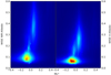 |
Fig. 5 Weighted density plots of the NEOWISE near-infrared (left) and visible (right) albedos vs. ML*. The cluster associated with rocky populations (ML* > 0) is more separated from the primitive cluster (ML* < 0) in the case of the near-infrared albedo, providing a better visual differentiation. |
4 Results and discussion
There are atotal of 104 collisional families with at least one member with determined ML* in the MOVIS catalog. In the following subsections we present the ML* distribution for 43 families detected in the MOVIS catalog, and for 27 of them, we also show the distributions of their associated backgrounds (see Sect. 4.3 for the definition of background). In addition, out of the 104 families, 17 of them present at least 40 asteroids that also have NEOWISE data, and 12 out of these 17 have at least 40 asteroids coincident with the SDSS MOC. We individually discuss some of them in the following sections.
4.1 The ML* distribution for the families in MOVIS
We compared the ML* distributions of the asteroid families present in the MOVIS database to the theoretical distributions computed in Sect. 3.1. The most efficient way to do this is through a Kolmogorov–Smirnov test (KS-test), since it is designed to compare samples of unidimensional probability distributions against a reference distribution (or against another sample). In addition, the KS-test works very well with a surprisingly small number of points in the sample (Stephens 1970).
The KS-test takes the cumulative distribution function (CDF) of the sample we want to compare (in our case, the ML* distribution of the family) and computes the maximum distance between this CDF and that of the reference distribution (the theoretical distributions that we computed). The test works under the initial hypothesis that the sample is drawn from the reference distribution. It is designed to reject this hypothesis whenever the maximum distance between the sample CDF and the reference CDF is higher than some critical value. It is important to note that failing to reject it does not confirm the initial hypothesis, but the test gives a good idea of how similar the two distributions are.
According to Stephens (1970), the KS-test serves a practical purpose for samples with NOBS ≥ 8. Therefore, we ran this test for all the families in the MOVIS catalog that have at least eight members and an error in the determination of ML* smaller than the first quartile of the full family sample (i.e.,  ). In Fig. 7 we present a graphical representation of the KS-test performed for the 43 families that fulfilled the previous requirements.
The results yielded rejections (with a confidence level of α =0.01, i.e., around 2.5σ) in all the cases for three of the four theoretical distributions that we proposed, except for nine families for which all the proposed distributions were rejected: Vesta, Hygiea, Themis, Nysa–Polana, Hilda, Erigone, Ino, Eos, and Ursula. For these families, we studied possible mixtures of the four distributions. These “theoretical” mixtures were created by generating random numbers according totwo (or more) of the computed distributions, up to the desired percentages (i.e., in a 25–75% P2–rocky mixture, 25% of the sample is generated according to a P2 distribution, and the other 75% is generated according to a rocky distribution).
Among the rest of the analyzed families, 5 of them are compatible with the P1 population, 10 are compatible with a P2 population, and 19 are compatible with our rocky distribution (see Table 3).
According to these results, we are able to characterize a family as belonging to one of the four proposed distributions by rejecting the other three. In other words, the result of the test gives an idea of how homogeneous a family is. It is interesting to note that the four distributions are rejected for some of the cases where the number of objects is high: for example, the Vesta family, with 408 objects in the analyzed distribution, known to be composed of basaltic asteroids, is rejected by this test as a 100% basaltic population. This tells us that when we have enough data, we are able to distinguish inhomogeneities in the family distributions. We discuss some of these cases in Sect. 4.2.
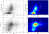 |
Fig. 6 Top: scatter plot (left) and corresponding weighted density plot (right) of the computed ML* from this work and near-infrared albedo values from NEOWISE, for a total of 8746 objects. Bottom: same as top panels, but for the computed a* from SDSS MOC (2210 objects). Overplotted in white are the points (with their error bars) corresponding to the mean values of these parameters for some of the families observed within MOVIS: 1 – Vesta, 2 – Flora, 3 – Eunomia, 4 – Themis, 5 – Nysa–Polana, 6 – Koronis, 7 – Eos. |
 |
Fig. 7 Cumulative distribution functions (CDFs) for all the families with NOBS ≥ 8 observed in MOVIS and |

Results from the Kolmogorov–Smirnov test for all the families that have NOBS ≥ 8 with  .
.
4.2 Individual families
4.2.1 Vesta (and Ino)
The Vesta family is one of the best known asteroid families, closely related to one of the largest asteroids within the solar system, (4) Vesta. This family presents characteristic high albedos (⟨pNIR⟩ = 0.52 ± 0.17), and is associated with the howardite-eucrite-diogenite (HED) meteorites (McCord et al. 1970; Binzel & Xu 1993; Moskovitz et al. 2010; Mayne et al. 2011).
As we mentioned in the previous section, the KS-test rejects the hypothesis that the Vesta family distribution comes from our theoretical basaltic population. According to Licandro et al. (2017), around 85% of the Vesta family members are V-types, and just 1–2% are classified as primitive objects. Using this information, we created new theoretical distributions by combining our basaltic, rocky, and primitive populations in different proportions. We then applied the KS-test to the ML* distribution of the Vesta family and these new distributions, looking for the combination that minimized the KS-test result and that was not rejected. The best result was obtained with a combination of 93% basaltic population and 7% rocky–primitive populations, in good agreement with the values obtained by Licandro et al. (2017).
When we add NEOWISE (Fig. C.1a) or SDSS data (Fig. C.1a) to our ML* parameter and create the corresponding weighted density plots, we can see that the Vesta family is unique, as we do not find this type of clustering in any of the other represented families. However, we can see in these plots the same behavior that we observed with just the analysis of the ML* distribution: a small contamination of rocky objects, which might be part of the background in that region of the asteroid belt, and even primitive asteroids, probably interlopers from the small primitive background in the inner belt.
One interesting case to mention together with Vesta is the Ino family. This family’s ML* CDF (see Fig. 7), although constructed from a small number of objects (just 11), shows a behavior that is quite strange. The KS-test rejects compatibilities with any of the four proposed theoretical distributions, even with distributions created from combinations of P1-P2-rocky populations. However, considering that the KS-test results were smaller for the comparisons with the rocky and basaltic populations, we decided to create combinations of these two and compare the resulting distributions with the family distribution: we minimized the KS-statistic for a mixture of 60% rocky and 40% basaltic populations. Nevertheless, the test also finds compatibilities for mixed samples of 50–50% up to 73–27% rocky–basaltic populations. Interestingly, Licandro et al. (2017) found that two of the V-type asteroids identified in the central main belt (180703) and (197480), belong to the Ino collisional family. Spectroscopic observations of a significant number of asteroids in this family would be needed in order to check whether it presents more basaltic asteroids or not.
4.2.2 Nysa–Polana and Erigone
Using photometric data from visible filters, Tedesco et al. (1982) proposed that the Nysa family (now known as the Nysa–Polana complex) presented asteroids with pronounced differences in their colors, pointing to the idea of a differentiated parent body. Later, Cellino et al. (2001) presented visible spectra of 22 asteroid members of this family, finding evidence that this group was actually formed by two different clusters associated with asteroids (44) Nysa and (142) Polana, rather than being the result of the disruption of a common differentiated parent body. Subsequent studies have revealed the dynamical complexity of this particular region of the asteroid belt (Walsh et al. 2013; Milani et al. 2014; Dykhuis & Greenberg 2015).
The weighted density plot using ML* and pNIR from NEOWISE (see Fig. C.1f), shows two clearly separated clusters for the Nysa–Polana family. Although the ML* CDF of the Nysa–Polana complex is visually very similar to that of our rocky population (see Fig. 7), the KS-test rejects the four proposed populations, i.e., the statistics tell us that the Nysa–Polana complex is not composed solely of rocky objects. Thus, after trying several mixtures of primitive and rocky distributions, the KS-test is minimized for a 90–10% mixed population of rocky–P2 objects. This result is in good agreement with the literature, since the whole Nysa–Polana complex is composed of approximately 20 000 asteroids, while the Polana family has around 2000 members.
Another family that needs to be discussed here is Erigone. This family is classified as primitive. Masiero et al. (2015) computed visible and near-infrared albedos for ~50% of the members in the Erigone family, giving values compatible with this classification (⟨pV⟩ = 0.05 ± 0.01 and ⟨pNIR⟩ = 0.06 ± 0.01). This is also evident from our weighted density plot of ML* and pNIR for the family (see Fig. C.1i). Interestingly, we find that the ML* CDF of this family (computed with a total of 31 observations) falls in between the CDFs of the P2 and the rocky populations (see Fig. 7). When looking for the best-fitting mixed distribution, we found it for a combination of 44–56% P2–rocky populations (see Fig. 8). Morate et al. (2016) studied visible spectra of 103 members of the Erigone family, 14 of which did not have any albedo information, and 8 of which presented spectra compatible with the rocky population defined here. This translates into a percentage of approximately 57% of rocky interlopers contaminating the sample, most likely from the background, and is in good agreement with the fraction of rocky population we find as a best-fitting result of the family’s CDF.
A possible explanation for these results might be that since family membership lists are based on optical magnitude, brighter objects are preferentially selected: NEOWISE has a flat sensitivity with respect to albedo, and will miss the small, higher albedo objects that are included in the family membership; conversely, as MOVIS is based on reflected light, it will be preferentially sensitive to high albedo objects (because of the steep growth of the number of family members with decreasing diameter). This might suggest some physical evidence. However, we consider this 44–56% ratio as a preliminary finding, which should be addressed by spectroscopic surveys.
 |
Fig. 8 Cumulative distribution function of the Erigone ML* distribution (green). The P1 primitive and rocky theoretical distributions are depicted in blue and red, respectively, and the mixture in gray. It is easy to see that the Erigone CDF fails to follow any of them. However, the 44–56% mixture seems to accurately fit the family sample. |
4.2.3 Eos
The Eos family is, in a certain way, as distinctive as Vesta; it is the only one in the whole main belt classified as a K-type. This has been shown by means of spectroscopic observations (Mothé-Diniz et al. 2005, 2008). In Masiero et al. (2014) it is also shown that the Eos family can be easily addressed by their characteristic 3.4 μm albedos.
There are a total of 599 asteroids from the Eos family in the MOVIS catalog. Of these, we used 328 for the analysis of the ML* distribution. Visual inspection of the CDF of this family (see Fig. 7) tells us that it is different from our four proposed populations (and different from all the other families as well). This is confirmed by the KS-test, which rejects compatibility with all the theoretical distributions that we have defined in this work. When looking for an approximate composition of this family, we needed to combine the P1, P2, and rocky populations. We found the best fit for a 25–55–20% combination of these distributions (Fig. 9).
If we also use the near-infrared albedo from NEOWISE and the SDSS data, we are able to distinguish a different clustering from that of the rest of the families, located in what we call a transition region in the ML* vs. pNIR or a* (see Figs. 6 and C.1k and C.2d). We identify this region with a K-type population, since Eos is the only family that shows this spread in the weighted density plots. Thus, the mixture we found as the best fit for the ML* is equivalent to that of a K-type distribution.
Although the combination of the P2 and rocky distributions probably gives a result of a K-type population, there is still a non-negligible “contamination” of objects from a P1 distribution (we note that 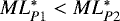 ). This is probably due to the family location in the outer belt where the proportion of primitive asteroids with negative slopes is higher than in the inner and middle regions.
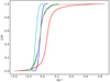 |
Fig. 9 Cumulative distribution function of the Eos ML* distribution(green), compared to the P1 (cyan), P2 (blue), and rocky (red) theoretical distributions. The mixed distribution which minimizes the KS-test (in gray) follows the family curve almost exactly. |
4.2.4 Baptistina
The Baptistina family has been the object of various studies during the last years. Some investigations pointed to a C-type low albedo family, inferred from the spectra of (298) Baptistina and some of its members. Subsequent studies have shown that this is not a typical homogeneous family: Reddy et al. (2011) linked Baptistina to Vesta and Flora, both nearby families in the proper element space (Baptistina is actually contained within Flora). Using albedos or SDSS data to separate these families does not provide definitive results (Masiero et al. 2013).
The KS-test is unable to distinguish the Baptistina family from a rocky population (see Table 3). However, after combining the ML* from MOVIS either with the pNIR or the a*, we are able to distinguish a two-cluster distribution for the Baptistina family (see Figs. C.1f and C.3g), different from the clustering present in the Flora family (see Figs. C.1b and C.2b). This kind of clustering might point to several scenarios: a fraction of the family may actually be composed of background asteroids; Baptistina may actually be formed of two different families, as is the case of the Nysa–Polana complex (Figs. C.1f and C.3g have cluster distributions similar to those in Figs. C.1f and C.2c); or this family may be the product of the breakup of a differentiated parent body.
Even if the KS-test failed to differentiate the Baptistina family CDF from that of a rocky family, after identifying this bimodality in the weighted density plots, we compared it to different combinations of primitive and rocky asteroids. We found the best approximation to the data for a combination of 83–17% rocky–P2 populations, which is in agreement with the two-cluster distribution found in Figs. C.1f and C.3g.
4.2.5 Some primitive families
After running the corresponding KS-tests on all the families, we found that four of them were rejected by the statistical test, despite visually presenting similar ML* distributions to those of P1 or P2 primitive populations. These families are Hygiea, Themis, Hilda, and Ursula. As in the previous cases, we looked for the combination of theoretical distributions that makes the test fail to reject it as a reference distribution, and then determined which distribution best fits the family data.
For Hygiea, this mixed distribution is composed of 67% P1 and 33% P2 populations. This is in agreement with data in the literature: Mothé-Diniz et al. (2001) showed that even though (10) Hygiea is one of the largest known C-type asteroids, a fraction of the objects in the family seem to belong to the Tholen B taxonomic class.
The situation for the Themis family is a bit different. It is similar to the Vesta case, in the sense that the CDF of the family follows almost exactly the CDF for the P1 population. As in the Vesta case, the proportion of one of the populations was extremely high with respect to the other: we found the best-fitting combination for a 95–5% mixture of P1–P2 distributions. This result, however, does not fully agree with the literature: Landsman et al. (2016) showed that this family, although composed of primitive asteroids, presents a diverse composition, and Fornasier et al. (2016) confirmed the spectral diversity within the Themis family. Here we report a slight contamination instead of a compositional variation.
In the case of the Hilda family, located within the Hilda dynamical group, the combination that minimizes the KS-test results is a 36–64% of P1–P2 populations. De Prá et al. (2018) reported a primitive surface composition with a bimodal distribution. This is in agreement with our results.
Information on the Ursula family is scarce, and the only compositional reference is found in Nesvorný et al. (2015), where they report Ursula to be a CX-type family, based on the SDSS colors of its members. For Ursula, the combination that we found is a 49–51% P1–P2, in agreement with the C–X classification from Nesvorný et al. (2015).
4.3 The background
It has been shown that large families have an associated halo of objects that presents similar properties to those of the main family, extending beyond the limits of the families determined using the traditional hierarchical clustering method (Parker et al. 2008; Carruba 2013; Brož & Morbidelli 2013). Apart from some recent efforts to include physical parameters in the identification of collisional families (Parker et al. 2008; Carruba et al. 2013; Masiero et al. 2013), this has long been a purely dynamical process, where the input variables for the family detection method are the proper orbital elements of the asteroids.
In addition to the family analyses, we performed a search on a rough approximation of the concept of halo, or family background. We wanted to check whether a family background (with a very relaxed definition) shares some physical properties with the main family, using the near-infrared colors in MOVIS: in our case, if the unidimensional (ML*) or bi-dimensional (ML* vs. pNIR or a*) distribution shows a similar behavior to that of the corresponding family. We define these backgrounds simply as the groups formed by the asteroids that do not belong to a family, but are located inside a cube in the 3D space of proper orbital elements centered around the mean values of semimajor axis, eccentricity, and sine of inclination of the main family and with an extension up to 3-σ of the mean.
We ran KS-tests comparing the ML* distribution of the backgrounds to that of their corresponding families. The background selection was performed using the same criteria as those in Sect. 4.1. Table 4 shows the results of these tests. From the 27 families analyzed, 23 backgrounds are, according to the KS-test, compatible with their associated families. The only backgrounds that the KS-test proves as being different from their corresponding families are Vesta, Flora, Adeona, and Mitidika.
If we look at Fig. 10, we can clearly see that the CDFs of Vesta and Flora show a different behavior from that of their backgrounds. This is mainly due to their nearby location in the asteroid belt: the Vesta background is clearly contaminated with a rocky population, coming probably from the entire background of the inner main belt; the Flora background is also contaminated, but with a basaltic population, due to its proximity to the Vesta family. The cases of Adeona and Mitidika are probably similar: they are located near two big rocky families, Eunomia and Juno. It is worth mentioning that the Baptistina family background, although compatible with the family, shows almost the same CDF as the Flora family background. This is, of course, because Baptistina is contained within Flora, and so they share the same background.
In addition to the unidimensional analysis, we also looked for similarities in family background using the near-infrared albedos (pNIR) and the a*. There are 17 families with more than 40 asteroids observed in MOVIS, coincident within the NEOWISE database, which also present at least ten coincident objects in the background. In the case of the coincidences with the SDSS database, there are just four familiesfulfilling the mentioned conditions: Vesta, Flora, Nysa–Polana, and Eos. The information provided is statistically less significant than that obtained using NEOWISE since there are fewer background coincidences than in the first case.
In Table A.2, we present mean values for the different family backgrounds in the MOVIS catalog. We note that most of the analyzed backgrounds share a similar distribution in the ML* vs. pNIR, and also in the ML* vs. a* space as their corresponding families. This is particularly interesting for the cases where the families are significantly different in composition from their surroundings:
Vesta. The background of the Vesta family seems to occupy the same region in the ML* vs. pNIR space as that occupied by the family (see Fig. C.1a), although there are objects with ML* and pNIR values similar to those shown by the Flora family, i.e., objects with rocky composition, as expected from the inner belt rock background.
Eos. This similarity is much more significant in this case. The Eos family is located in the outer belt, mainly populated by primitive objects having ML* < 0 and low albedos (pNIR < 0.1). But if we look at its background (Fig. C.1e), instead of this primitive population we find objects with a similar distribution to that of the family, suggesting that these objects are very likely related to Eos. This relationship had been previously noted using only SDSS data (Brož & Morbidelli 2013).
Nysa–Polana and Baptistina. The results in this case also point to a close relation between these backgrounds and their families since both families present a bimodal distribution of asteroids and their corresponding backgrounds seem to present the same behavior: two clusters related to the different compositions of the family members.
The information provided here points out, using near-infrared photometry alone (and also in combination with the pNIR from NEOWISE and a* from SDSS), that the family backgrounds are closely related to their family counterparts. This suggests further evidence of halos around the currently known families, confirming what has already been proposed by Parker et al. (2008), Carruba et al. (2013), and Masiero et al. (2013), among others: the definition of asteroid family needs to be updated including physical parameters to constrain family membership.
Results from the Kolmogorov–Smirnov test used to compare the families to their corresponding backgrounds.
 |
Fig. 10 Cumulative distribution functions for the 27 analyzed families (green) and their associated backgrounds (purple). The selected samples of background to analyze are drawn from the MOVIS database under the same conditions as the main family sample. The box in each plot shows the name of the family, and the number of objects from the family and from the background used for the analysis. |
5 Summary
In the present work, we have conducted an analysis on the families present in the MOVIS catalog. To perform this analysis, we have developed a near-infrared parameter, based on the Y − J and J− Ks colors. In order to define this parameter, we have used those objects with observations in the Y, J, and Ks filters, and with errors in their determination below different thresholds, testing several configurations to construct the final ML* definition (see Eq. (1)). We carried out our analysis combining this parameter with the near-infrared albedos from NEOWISE and the a* color from SDSS. Within the MOVIS catalog we have found 6299 asteroids, which belong to a total of 104 of the families defined in Nesvorný et al. (2015).
Using the ML*, we have identified four different distributions within the MOVIS data: P1 and P2 (associated with primitive asteroids, i.e., B-, C-, X-types, and subclasses), rocky (associated with S-types and subclasses), and basaltic(associated with V-types). We compared these distributions with those of the families with NOBS ≥ 8 and 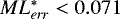 , using Kolmogorov–Smirnov tests. Out of the 43 analyzed families, we report 5 compatible with a P1 distribution, 10 compatible with a P2, and 19 compatible with a rocky population. The KS-test yielded rejections when comparing the other nine families with the four theoretical distributions. In these cases, we compared the families with mixed distributions, avoiding KS-test rejections for all of them. These results are summarized in Table 3. We note that, in general, for the families with a large number of objects, the trend is to be rejected by the KS-test, finding best fits using mixed distributions. This points to a general (although smooth) inhomogeneity in the family compositions.
We are confirming, using near-infrared photometry combined with NEOWISE and SDSS data, some results already known for several families. Vesta shows a small contamination of rocky and primitive asteroids (Licandro et al. 2017); Nysa–Polana presents a bimodality in its composition corresponding to the presence of two families (Cellino et al. 2001; Walsh et al. 2013; Milani et al. 2014; Dykhuis & Greenberg 2015); Eos is the only K-type family identified in the inner belt (Mothé-Diniz et al. 2005, 2008); and Hilda shows some bimodality inside the primitive region (De Prá et al. 2018). In addition, we found relevant results in our analysis related to the Ino and Baptistina families.
The Ino family shows a very different distribution of ML* compared tothe theoretical distributions that we propose, and also compared to all the other families; the best-fitting mixture is for a 60–40% rocky–basaltic combination. In addition, two of the V-type asteroids identified in Licandro et al. (2017) belong to this family. It would be very interesting to check if this composition is reflected in the spectroscopic data since there are no known basaltic families apart from Vesta.
Regarding the Baptistina family, if we use the data in the MOVIS catalog combined with the NEOWISE near-infrared albedos, we find that it presents a two-cluster distribution within the ML* vs. pNIR space. By comparing the ML* distribution of Baptistina to that of a mixture of two theoretical populations, we find the best fit for a combination of 83–17% rocky-P2; in other words, the ML* confirms this bimodality by itself. This can be explained if this family is the result of the breakup of a differentiated parent body (which would be unique to the main asteroid belt). Otherwise, this family presents high contamination from the Flora family rocky background. It can also be hypothesized that Baptistina is actually formed of two families, one formed of high-albedo rocky objects, and the other composed of primitive asteroids with moderately low albedos.
Finally, we used Kolmogorov–Smirnov tests to compare the background populations that we defined against their associated families. We report compatibilities between the families and their backgrounds in 23 out of the 27 studied cases (see Table 4). We show that the surrounding objects usually have a similar composition to that of the main family. This provides further evidence for the necessity of an update in the definitions of asteroid families: using only dynamical elements to address family membership will not give results that are as accurate as those that we would be able to obtain if we also took into account physical properties, such as the albedo, photometry, or even spectroscopy, whenever available.
Acknowledgements
DM gratefully acknowledges the Spanish Ministry of Economy and Competitiveness (MINECO) for the financial support received in the form of a Severo-Ochoa PhD fellowship, within the Severo-Ochoa International PhD Program. All the authors acknowledge support from the AYA2015-67772-R (MINECO, Spain), and from the Instituto de Astrofísica de Canarias. JdL acknowledges financial support from MINECO under the 2015 Severo Ochoa Program MINECO SEV-2015-0548. The work of MP was also supported by a grant from the Romanian National Authority for Scientific Research – UEFISCDI, project number PN-III-P1-1.2-PCCDI-2017-0371. The authors would also like to thank the referee for the comments and suggestions that helped to improve this article.
Appendix A Additional tables
Mean values of ML* computed forthe different families present in the MOVIS catalog.
Mean ML*, pNIR, and a* for the background populations of the families with more than 40 asteroids observed in MOVIS, and with more than 10 asteroids in coincidence with the SDSS and NEOWISE databases.
Appendix B Auxiliary figures
 |
Fig. B.1 Graphical representation of the results of the fits for the case where we assumed three distributions: three Gaussians (left), three Lorentzians (center), one Gaussian for the primitive population and two Lorentzians for both rocky and basaltic populations (right). The upper plots represent the probability density functions associated with the ML* distributions. The lower plots are the corresponding cumulative distribution functions. |
 |
Fig. B.2 Same as Fig. B.1, but with four distributions: four Gaussians (left), four Lorentzians (center), two Gaussians for the two primitive populations, and two Lorentzians for both rocky and basaltic populations (right). We can see that the combinations in the right panels of Figs. B.1 and B.2 fit the observations accurately. |
 |
Fig. B.3 CDFs of the theoretical distributions defined for the case of a three-population fit and those defined for a four-population fit, compared to the primitive families with the highest number of objects in the MOVIS catalog (Hygiea and Themis). In the upper plots we show the three-population case (primitive in cyan, rocky in red, basaltic in black). The lower plots show the four-population case (P1 in blue, P2 in cyan). |
Appendix C Density plots of the detected families
 |
Fig. C.1 Asteroid families detected within the MOVIS catalog, with at least 40 coincidences with NEOWISE, and with a background of at least ten asteroids. In these plots we represent ML* vs. pNIR. On the left, we represent the observed family, and on the right the background we defined for that same family. Upper plots are weighted density plots (see text for explanation), and lower plots are scatter representations of the observed asteroids, with the corresponding error bars. |
 |
Fig. C.2 Asteroid families detected within the MOVIS catalog, with at least 40 coincidences with SDSS, and with a background of at least ten asteroids. In these plots we represent ML* vs. a*. |
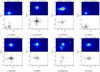 |
Fig. C.3 ML* vs. a* for the asteroid families detected within the MOVIS catalog, with at least 40 coincidences with SDSS, and without a background (or the background that we defined had less than ten coincident asteroids with SDSS). |
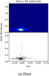 |
Fig. C.4 ML* vs. pNIR for Dora, the only asteroid family in the MOVIS catalog with at least 40 coincidences with NEOWISE, and without a background (or the background that we defined had less than ten coincident asteroids with NEOWISE). |
References
- Bessell, M. S. 2005, ARA&A, 43, 293 [NASA ADS] [CrossRef] [Google Scholar]
- Binzel, R. P., & Xu, S. 1993, Science, 260, 186 [NASA ADS] [CrossRef] [Google Scholar]
- Bottke, Jr., W. F., Vokrouhlický, D., Rubincam, D. P., & Broz, M. 2002, The Effect of Yarkovsky Thermal Forces on the Dynamical Evolution of Asteroids and Meteoroids, eds. W. F. Bottke, Jr., A. Cellino, P. Paolicchi, & R. P. Binzel (Tucson: University of Arizona Press), 395 [Google Scholar]
- Brož, M., & Morbidelli, A. 2013, Icarus, 223, 844 [NASA ADS] [CrossRef] [Google Scholar]
- Brož, M., Morbidelli, A., Bottke, W. F., et al. 2013, A&A, 551, A117 [NASA ADS] [CrossRef] [EDP Sciences] [Google Scholar]
- Carruba, V. 2013, MNRAS, 431, 3557 [NASA ADS] [CrossRef] [Google Scholar]
- Carruba, V., Domingos, R. C., Nesvorný, D., et al. 2013, MNRAS, 433, 2075 [NASA ADS] [CrossRef] [EDP Sciences] [Google Scholar]
- Carvano, J. M., Hasselmann, P. H., Lazzaro, D., & Mothé-Diniz, T. 2010, A&A, 510, A43 [NASA ADS] [CrossRef] [EDP Sciences] [Google Scholar]
- Cellino, A., Zappalà, V., Doressoundiram, A., et al. 2001, Icarus, 152, 225 [NASA ADS] [CrossRef] [Google Scholar]
- De Prá, M. N., Pinilla-Alonso, N., Carvano, J. M. F., et al. 2018, Icarus, 311, 35 [NASA ADS] [CrossRef] [Google Scholar]
- DeMeo, F. E., & Carry, B. 2013, Icarus, 226, 723 [NASA ADS] [CrossRef] [Google Scholar]
- DeMeo, F. E., Binzel, R. P., Slivan, S. M., & Bus, S. J. 2009, Icarus, 202, 160 [NASA ADS] [CrossRef] [Google Scholar]
- Doressoundiram, A., Barucci, M. A., Fulchignoni, M., & Florczak, M. 1998, Icarus, 131, 15 [NASA ADS] [CrossRef] [Google Scholar]
- Dykhuis, M. J., & Greenberg, R. 2015, Icarus, 252, 199 [NASA ADS] [CrossRef] [Google Scholar]
- Florczak, M., Barucci, M. A., Doressoundiram, A., et al. 1998, Icarus, 133, 233 [NASA ADS] [CrossRef] [Google Scholar]
- Florczak, M., Lazzaro, D., Mothé-Diniz, T., Angeli, C. A., & Betzler, A. S. 1999, A&AS, 134, 463 [NASA ADS] [CrossRef] [EDP Sciences] [Google Scholar]
- Fornasier, S., Lantz, C., Perna, D., et al. 2016, Icarus, 269, 1 [NASA ADS] [CrossRef] [Google Scholar]
- Gil-Hutton, R. 2006, Icarus, 183, 93 [NASA ADS] [CrossRef] [Google Scholar]
- Ishihara, D., Onaka, T., Kataza, H., et al. 2010, A&A, 514, A1 [NASA ADS] [CrossRef] [EDP Sciences] [Google Scholar]
- Ivezić, Ž., Tabachnik, S., Rafikov, R., et al. 2001, AJ, 122, 2749 [NASA ADS] [CrossRef] [Google Scholar]
- Ivezić, Ž., Lupton, R. H., Jurić, M., et al. 2002, AJ, 124, 2943 [NASA ADS] [CrossRef] [Google Scholar]
- Jarrett, T. H., Cohen, M., Masci, F., et al. 2011, ApJ, 735, 112 [NASA ADS] [CrossRef] [Google Scholar]
- Kaiser, N., Burgett, W., Chambers, K., et al. 2010, in Ground-based and Airborne Telescopes III, Proc. SPIE, 7733, 77330E [Google Scholar]
- Landsman, Z. A., Licandro, J., Campins, H., et al. 2016, Icarus, 269, 62 [NASA ADS] [CrossRef] [Google Scholar]
- Licandro, J., Popescu, M., Morate, D., & de León J. 2017, A&A, 600, A126 [NASA ADS] [CrossRef] [EDP Sciences] [Google Scholar]
- Mainzer, A., Grav, T., Bauer, J., et al. 2011, ApJ, 743, 156 [NASA ADS] [CrossRef] [Google Scholar]
- Mainzer, A., Bauer, J., Cutri, R. M., et al. 2014, ApJ, 792, 30 [NASA ADS] [CrossRef] [Google Scholar]
- Masiero, J. R., Mainzer, A. K., Grav, T., et al. 2011, ApJ, 741, 68 [NASA ADS] [CrossRef] [Google Scholar]
- Masiero, J. R., Mainzer, A. K., Bauer, J. M., et al. 2013, ApJ, 770, 7 [NASA ADS] [CrossRef] [Google Scholar]
- Masiero, J. R., Grav, T., Mainzer, A. K., et al. 2014, ApJ, 791, 121 [NASA ADS] [CrossRef] [Google Scholar]
- Masiero, J. R., DeMeo, F. E., Kasuga, T., & Parker, A. H. 2015, Asteroid Family Physical Properties, eds. P. Michel, F. E. DeMeo, & W. F. Bottke (Tucson: University of Arizona Press), 323 [Google Scholar]
- Mayne, R. G., Sunshine, J. M., McSween, H. Y., Bus, S. J., & McCoy, T. J. 2011, Icarus, 214, 147 [NASA ADS] [CrossRef] [Google Scholar]
- McCord, T. B., Adams, J. B., & Johnson, T. V. 1970, Science, 168, 1445 [NASA ADS] [CrossRef] [PubMed] [Google Scholar]
- McMahon, R. G., Banerji, M., Gonzalez, E., et al. 2013, Messenger, 154, 35 [Google Scholar]
- Milani, A., Cellino, A., Knežević, Z., et al. 2014, Icarus, 239, 46 [NASA ADS] [CrossRef] [Google Scholar]
- Morate, D., de León, J., De Prá, M., et al. 2016, A&A, 586, A129 [NASA ADS] [CrossRef] [EDP Sciences] [Google Scholar]
- Moskovitz, N. A., Willman, M., Burbine, T. H., Binzel, R. P., & Bus, S. J. 2010, Icarus, 208, 773 [NASA ADS] [CrossRef] [Google Scholar]
- Mothé-Diniz, T., di Martino, M., Bendjoya, P., Doressoundiram, A., & Migliorini, F. 2001, Icarus, 152, 117 [NASA ADS] [CrossRef] [Google Scholar]
- Mothé-Diniz, T., Roig, F., & Carvano, J. M. 2005, Icarus, 174, 54 [NASA ADS] [CrossRef] [Google Scholar]
- Mothé-Diniz, T., Carvano, J. M., Bus, S. J., Duffard, R., & Burbine, T. H. 2008, Icarus, 195, 277 [NASA ADS] [CrossRef] [Google Scholar]
- Nesvorny, D. 2010, NASA Planetary Data System, 133 [Google Scholar]
- Nesvorny, D. 2012, NASA Planetary Data System, 189 [Google Scholar]
- Nesvorný, D., Jedicke, R., Whiteley, R. J., & Ivezić, Ž. 2005, Icarus, 173, 132 [NASA ADS] [CrossRef] [Google Scholar]
- Nesvorný, D., Brož, M., & Carruba, V. 2015, Identification and Dynamical Properties of Asteroid Families, eds. P. Michel, F. E. DeMeo, & W. F. Bottke (Tucson: University of Arizona Press), 297 [Google Scholar]
- Newville, M., Stensitzki, T., Allen, D. B., & Ingargiola, A. 2014, LMFIT: Non-Linear Least-Square Minimization and Curve-Fitting for Python [Google Scholar]
- Novaković, B., Cellino, A., & Knežević Z. 2011, Icarus, 216, 69 [NASA ADS] [CrossRef] [Google Scholar]
- Parker, A., Ivezić, Ž., Jurić, M., et al. 2008, Icarus, 198, 138 [NASA ADS] [CrossRef] [Google Scholar]
- Popescu, M., Licandro, J., Morate, D., et al. 2016, A&A, 591, A115 [NASA ADS] [CrossRef] [EDP Sciences] [Google Scholar]
- Popescu, M., Licandro, J., Carvano, J. M. F., et al. 2018, A&A, 617, A12 [NASA ADS] [CrossRef] [EDP Sciences] [Google Scholar]
- Reddy, V., Carvano, J. M., Lazzaro, D., et al. 2011, Icarus, 216, 184 [NASA ADS] [CrossRef] [Google Scholar]
- Skrutskie, M. F., Cutri, R. M., Stiening, R., et al. 2006, AJ, 131, 1163 [NASA ADS] [CrossRef] [Google Scholar]
- Stephens, M. 1970, J. R. Stat. Soc. Ser. B, 32, 115 [Google Scholar]
- Sutherland, W., Emerson, J., Dalton, G., et al. 2015, A&A, 575, A25 [NASA ADS] [CrossRef] [EDP Sciences] [Google Scholar]
- Tedesco, E. F., Gradie, J., Tholen, D. J., & Zellner, B. 1982, in BAAS, 14, 720 [NASA ADS] [Google Scholar]
- Vokrouhlický, D., Brož, M., Morbidelli, A., et al. 2006, Icarus, 182, 92 [NASA ADS] [CrossRef] [Google Scholar]
- Walsh, K. J., Delbó, M., Bottke, W. F., Vokrouhlický, D., & Lauretta, D. S. 2013, Icarus, 225, 283 [NASA ADS] [CrossRef] [Google Scholar]
- Waskom, M., Botvinnik, O., O’Kane, D., et al. 2017, mwaskom/seaborn: v0.8.1 [Google Scholar]
- Wright, E. L., Eisenhardt, P. R. M., Mainzer, A. K., et al. 2010, AJ, 140, 1868 [NASA ADS] [CrossRef] [Google Scholar]
- York, D. G., Adelman, J., Anderson, Jr., J. E., et al. 2000, AJ, 120, 1579 [CrossRef] [Google Scholar]
The published version of the catalog can be found at http://vizier.u-strasbg.fr/viz-bin/VizieR-3?-source=J/A%2bA/591/A115/movis-c
All Tables
Central wavelengths and passbands for the different filters used in the SDSS (Bessell 2005), VISTA-VHSa, and NEOWISE (Jarrett et al. 2011) surveys.
Mean ML* values computed for the four different populations detected within the ML* distribution.
Results from the Kolmogorov–Smirnov test for all the families that have NOBS ≥ 8 with .
Results from the Kolmogorov–Smirnov test used to compare the families to their corresponding backgrounds.
Mean values of ML* computed forthe different families present in the MOVIS catalog.
Mean ML*, pNIR, and a* for the background populations of the families with more than 40 asteroids observed in MOVIS, and with more than 10 asteroids in coincidence with the SDSS and NEOWISE databases.
All Figures
|
Fig. 1 Response curves of the Y, J, H, and Ks VISTA filters (blue), together with the DeMeo et al. (2009) template spectra of the asteroid populations in our study. We averaged the templates for the B-, C-, and X-types and subclasses (primitives); the S-types and subclasses (rocky); and V-types (basaltic). The template spectra have been normalized to unity at 1.25 μm (central wavelength of the J filter) for representation purposes. |
| In the text | |
|
Fig. 2 Proper semimajor axis vs. proper inclination (left panel) and proper eccentricity (right panel) for the asteroids observed within MOVIS catalog. The blue background represents the full sample of objects with Y − J and J− Ks colors defined in MOVIS (a total of 18 263 objects). In orange, we overplot those asteroids belonging to families (6299 objects). |
| In the text | |
|
Fig. 3 Graphical representation of the procedure followed to parametrize the near-infrared colors in MOVIS. The left panel shows the kernel density estimation plot of the J− Ks (JmK) vs. Y −J (YmJ) distributions. Brighter regions correspond to higher density of points. The straight line connects the two main cluster centers (peaks of maximum density). The third cluster (Y − J >0.5) corresponds to basaltic asteroids (Popescu et al. 2016). The right panel shows the univariate PDF estimation for the ML* before the computation of the required offset to set the separation between the rocky and primitive asteroids clusters at the origin. The vertical black line indicates the point where the PDF density is minimum between the two maxima. We used the C0.10 subset for this example. |
| In the text | |
|
Fig. 4 Histograms and fits for the ML* distribution. We have used only those objects presenting an error in the computation of ML* smaller than the first quartile of the full sample ( |
| In the text | |
|
Fig. 5 Weighted density plots of the NEOWISE near-infrared (left) and visible (right) albedos vs. ML*. The cluster associated with rocky populations (ML* > 0) is more separated from the primitive cluster (ML* < 0) in the case of the near-infrared albedo, providing a better visual differentiation. |
| In the text | |
|
Fig. 6 Top: scatter plot (left) and corresponding weighted density plot (right) of the computed ML* from this work and near-infrared albedo values from NEOWISE, for a total of 8746 objects. Bottom: same as top panels, but for the computed a* from SDSS MOC (2210 objects). Overplotted in white are the points (with their error bars) corresponding to the mean values of these parameters for some of the families observed within MOVIS: 1 – Vesta, 2 – Flora, 3 – Eunomia, 4 – Themis, 5 – Nysa–Polana, 6 – Koronis, 7 – Eos. |
| In the text | |
|
Fig. 7 Cumulative distribution functions (CDFs) for all the families with NOBS ≥ 8 observed in MOVIS and |
| In the text | |
|
Fig. 8 Cumulative distribution function of the Erigone ML* distribution (green). The P1 primitive and rocky theoretical distributions are depicted in blue and red, respectively, and the mixture in gray. It is easy to see that the Erigone CDF fails to follow any of them. However, the 44–56% mixture seems to accurately fit the family sample. |
| In the text | |
|
Fig. 9 Cumulative distribution function of the Eos ML* distribution(green), compared to the P1 (cyan), P2 (blue), and rocky (red) theoretical distributions. The mixed distribution which minimizes the KS-test (in gray) follows the family curve almost exactly. |
| In the text | |
|
Fig. 10 Cumulative distribution functions for the 27 analyzed families (green) and their associated backgrounds (purple). The selected samples of background to analyze are drawn from the MOVIS database under the same conditions as the main family sample. The box in each plot shows the name of the family, and the number of objects from the family and from the background used for the analysis. |
| In the text | |
|
Fig. B.1 Graphical representation of the results of the fits for the case where we assumed three distributions: three Gaussians (left), three Lorentzians (center), one Gaussian for the primitive population and two Lorentzians for both rocky and basaltic populations (right). The upper plots represent the probability density functions associated with the ML* distributions. The lower plots are the corresponding cumulative distribution functions. |
| In the text | |
|
Fig. B.2 Same as Fig. B.1, but with four distributions: four Gaussians (left), four Lorentzians (center), two Gaussians for the two primitive populations, and two Lorentzians for both rocky and basaltic populations (right). We can see that the combinations in the right panels of Figs. B.1 and B.2 fit the observations accurately. |
| In the text | |
|
Fig. B.3 CDFs of the theoretical distributions defined for the case of a three-population fit and those defined for a four-population fit, compared to the primitive families with the highest number of objects in the MOVIS catalog (Hygiea and Themis). In the upper plots we show the three-population case (primitive in cyan, rocky in red, basaltic in black). The lower plots show the four-population case (P1 in blue, P2 in cyan). |
| In the text | |
|
Fig. C.1 Asteroid families detected within the MOVIS catalog, with at least 40 coincidences with NEOWISE, and with a background of at least ten asteroids. In these plots we represent ML* vs. pNIR. On the left, we represent the observed family, and on the right the background we defined for that same family. Upper plots are weighted density plots (see text for explanation), and lower plots are scatter representations of the observed asteroids, with the corresponding error bars. |
| In the text | |
|
Fig. C.2 Asteroid families detected within the MOVIS catalog, with at least 40 coincidences with SDSS, and with a background of at least ten asteroids. In these plots we represent ML* vs. a*. |
| In the text | |
|
Fig. C.3 ML* vs. a* for the asteroid families detected within the MOVIS catalog, with at least 40 coincidences with SDSS, and without a background (or the background that we defined had less than ten coincident asteroids with SDSS). |
| In the text | |
|
Fig. C.4 ML* vs. pNIR for Dora, the only asteroid family in the MOVIS catalog with at least 40 coincidences with NEOWISE, and without a background (or the background that we defined had less than ten coincident asteroids with NEOWISE). |
| In the text | |
Current usage metrics show cumulative count of Article Views (full-text article views including HTML views, PDF and ePub downloads, according to the available data) and Abstracts Views on Vision4Press platform.
Data correspond to usage on the plateform after 2015. The current usage metrics is available 48-96 hours after online publication and is updated daily on week days.
Initial download of the metrics may take a while.