| Issue |
A&A
Volume 617, September 2018
|
|
|---|---|---|
| Article Number | A60 | |
| Number of page(s) | 23 | |
| Section | Interstellar and circumstellar matter | |
| DOI | https://doi.org/10.1051/0004-6361/201730639 | |
| Published online | 13 September 2018 | |
Chemical modeling of internal photon-dominated regions surrounding deeply embedded HC/UCHII regions
1
I. Physikalisches Institut, Universität zu Köln,
Zülpicher Strasse 77,
50937
Köln,
Germany
e-mail: This email address is being protected from spambots. You need JavaScript enabled to view it.
2
LERMA, Observatoire de Paris,
5 place Jules Janssen,
92190
Meudon,
France
3
Université Paris Diderot, Sorbonne Paris Cité,
75013
Paris,
France
4
Max-Planck-Institut für extraterrestrische Physik,
Giessenbachstrasse 1,
85748
Garching bei München,
Germany
Received:
16
February
2017
Accepted:
7
February
2018
Abstract
Aims. We aim to investigate the chemistry of internal photon-dominated regions (PDRs) surrounding deeply embedded hypercompact (HC) and ultracompact (UC) HII regions. We search for specific tracers of this evolutionary stage of massive star formation that can be detected with current astronomical facilities.
Methods. We modeled hot cores with embedded HC/UCHII regions (called HII region models in the article despite the fact that we do not model the HII region itself), by coupling the astrochemical code Saptarsy to a radiative transfer framework obtaining the spatio-temporal evolution of abundances as well as time-dependent synthetic spectra. In these models where we focused on the internal PDR surrounding the HII region, the gas temperature is set to the dust temperature and we do not include dynamics thus the density structure is fixed. We compared this to hot molecular core (HMC) models and studied the effect on the chemistry of the radiation field which is included in the HII region models only during the computation of abundances. In addition, we investigated the chemical evolution of the gas surrounding HII regions with models of different densities at the ionization front, different sizes of the ionized cavity and different initial abundances.
Results. We obtain the time evolution of synthetic spectra for a dozen of selected species as well as ratios of their integrated intensities. We find that some molecules such as C, N2H+, CN, and HCO do not trace the inner core and so are not good tracers to distinguish the HII/PDR regions to the HMCs phase. On the contrary, C+ and O trace the internal PDRs, in the two models starting with different initial abundances, but are unfortunately currently unobservable with the current achievable spatial resolution because of the very thin internal PDR (Δ rPDR < 100 AU). The emission of these two tracers is very dependent on the size of the HII region and on the density in the PDR. In addition, we find that the abundance profiles are highly affected by the choice of the initial abundances, hence the importance to properly define them.
Key words: astrochemistry / stars: formation / stars: massive / ISM: molecules / ISM: lines and bands / evolution
Current affiliation: Department of Chemistry, University of Virginia, McCormick Road, Charlottesville, VA 22904, USA.
© ESO 2018
1 Introduction
The chemical evolution of hot molecular cores (HMCs) has been the focus of many studies (Garrod & Herbst 2006; Vasyunin & Herbst 2013; Garrod 2013) as these objects often present a very rich and complex chemistry. HMCs are compact (≤0.10 pc), very dense (nH ≥ 106 cm−3), hot (T ≥ 100 K) and are a characteristic early stage of massive star formation (Kurtz et al. 2000). They are transient objects with a lifetime, although not well constrained, of about 104–105 yr (Herbst & van Dishoeck 2009). It is still unclear if they are formed before the hyper compact HII (HCHII) region stage or coexist with it (Gaume et al. 1995; Kurtz 2005; Beuther et al. 2007). HCHII regions are compact (<0.01 pc) and very dense (>106 cm−3) ionized gas regions (with Te ~ 104 K) surrounding recently born high-mass stars still deeply embedded in their parental clouds (e.g., Kurtz et al. 2000; Hoare et al. 2007; Sánchez-Monge et al. 2013b). The small sizes are likely due to the high accretion rates and high densities of the first evolutionary stages. HCHII regions are expected to evolve into ultracompact HII (UCHII) regions as the embedded proto-star(s) become more luminous and gradually ionize their surroundings, and the accretion rates and surrounding density decrease. This evolution is not necessarily homogeneous as HII regions may flicker as proposed theoretically by Peters et al. (2010a,b) and found observationally by De Pree et al. (2014). UCHII regions are slightly larger (0.1 pc) with densities of about 104 cm−3 (e.g., Wood & Churchwell 1989; Kurtz 2005).
The small size of HC and UCHII regions results in very strong ultraviolet (UV) radiation fields at the ionization front, that is, at the interface between the ionized gas and the molecular gas. This results in photon-dominated regions (PDRs) formed at the border between the HII region and the molecular dense cloud where they are embedded. These so-called internal PDRs are very dense (nH ≥ 106 cm−3) and very thin because of the fast decrease of the radiation field (Δ rPDR ≈ 200 AU, corresponding to AV = 1.6 mag obtained with the standard Milky Way extinction curve). Most chemical models do not extend their studies to the evolutionarystages associated with HCHII and UCHII regions. So far, only a few studies have investigated internal PDRs (e.g., Bruderer et al. 2009a,b; Lee et al. 2015) in the case of an outflow cavity around low-mass stars with weak UV fields.
Observationally, HMCs and deeply embedded HC and UCHII regions have comparable spectral energy distributions in the infrared (IR) and sub-mm regime (e.g., Churchwell 2002; Cesaroni et al. 2015). However during the HMC phase the proto-star is not sufficiently evolved and does not radiate large enough quantities of UV photons to have a bright free-free thermal emission from ionized gas. Thus, HMCs are weak or even unobservable in the radio-continuum regime (Hoare et al. 2007; Beuther et al. 2007). This is the main observational difference between these two evolutionary stages of massive star formation. Do other observational methods perform better in differentiating these two phases? Can these phases be characterized by some specific chemical tracers? Can the presence of the internal PDRs be detected and how?
In this work we study the chemistry of the gas associated with HC/UCHII regions and their internal PDRs, without looking at the emission from the gas in the ionized cavity but only the gas in the PDR, as well as in HMCs before they are largely affected by UV radiation. We study the spatio-temporal evolution of the radiation field in HII region models as well as the evolution of the dust temperature, and how these physical parameters affect the chemistry and emissivity of different atomic and molecular tracers. Density is a parameter fixed in time in these models but we investigate the variation in the chemistry due to the density at the ionization front (i.e., density in the neutral gas just beyond the front), the different sizes of the ionized cavity, the density structure and the initial elementary abundances.
The paper is structured as follows: In Sect. 2 we describe the HMC and HII regions models, the physical parameters as well as the chemical code and the different modifications implemented since the first paper: Choudhury et al. (2015). In Sect. 3 we present first the different models as well as the temperature and radiation field intensity variations. Then we present the spatio-temporal evolution of abundances for selected species, the dissociation front properties derived from H2 abundances and the line emission of the selected species. The results are finally discussed in Sect. 4. Finally we summarize our findings in Sect. 5 and give some future directions for this work.
2 Method
The chemical modeling was performed with Saptarsy (see Sect. 2.3 and Choudhury et al. 2015). Saptarsy works alongside RADMC-3D1 (Dullemond 2012) through a Python based wrapper script (Choudhury et al. 2015), chemical mode of a former version of the framework Pandora2 (Schmiedeke et al. 2016). This was done to obtain synthetic spectra using the detailed modeling of the spatio-temporal evolution of the chemical abundances. The modeling framework is presented in the flowchart in Fig. 1 and is summarized as follows: first, based on a density profile and the evolution of stellar parameters, RADMC-3D calculates both the dust temperature and the mean intensity of the radiation field self-consistently. The gas temperature is assumed to be equal to the dust temperature in all models. This approximation will be lifted in a future work since it is known that the gas temperature may be much higher than the dust temperature at the inner edge of the PDR as well as in low density environments such as the envelope in our models (Lesaffre et al. 2005). In a second step, the spatial evolution of the density and the spatio-temporal evolution of the dust temperature and radiation field intensity are used by Saptarsy to compute relative abundances. Finally, we used the abundances as inputs for RADMC-3D to produce time-dependent synthetic spectra using the LTE approximation. The spectra can then be post-processed (convolved) to be compared to observations. The structure of the models and the chemical code are described in more detail below.
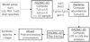 |
Fig. 1 Flowchart showing the setup of the variant of the modeling framework Pandora (Schmiedeke et al. 2016) employed here. |
2.1 HMC, Hollow HMC and HII region models
HMCs are modeled as spherical symmetric cores containing a single central protostar. The star is surrounded by gas and dust3 with a density profile defined as follows:
 (1)
(1)
where nc is the central density and rp is the size of the inner flat portion of the density profile. The exponent γ defines the steepness of the Plummer-like function.
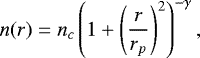
The HII region and its surroundings4 are modeledas if they were an HMC (see above) with a spherical cavity around the proto-star filled only with ionized hydrogen and electrons uniformly distributed, in other words, a Strömgren sphere (see also Schmiedeke et al. 2016). In Fig. 2 we represent an HII region with its real geometry (light blue) and its geometry as modeled in this work (dark blue). The cavity is assumed to be dust free, the spatial distribution of the dust remains unknown for HC/UCHII regions and models of more evolved HII regions suggest that big grains such as the ones used in this work are swept out of the cavity (Akimkin et al. 2015). But we notethat if radiation pressure pushes the grains out of the HII region, then the PDR will have enhanced dust opacity.
In orderto compare the chemical evolution of HMCs and HII regions we created a third set of models called “Hollow HMC” (hereafter HHMC). The HHMC model has the same density structure as the HMC model, but it contains a cavity in the center matching the size of the HII region cavity. With this artifice we ensure that the density profile as well as the total column density are the same as in the HII region models. Similarly, the temperatureprofile in the HHMC and HII region models are the same. Thus, the line emission in these two models is directly comparable. The difference between the HII region model and the HHMC model is the emission of UV photonsfrom the proto-star, which is modeled in Saptarsy with the implementation of the spatio-temporal evolution of the radiation field in the HII region model. Therefore, we can focus on the effect of the radiation field on the chemistry and line emission of several selected species. In Fig. 3 we show a scheme for the three models and their characteristics.
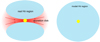 |
Fig. 2 Left: sketch of the real geometry of the HII region in the presence of accretion (based on models by Peters et al. 2010a,b). Right: our approximation by a spherical HII region filled with electrons and ions, but no dust. The PDR and the molecular gas surrounding the HII region are not represented in the sketches. Since the accretion disk does not cover a large fraction of the volume, and does not shield a large part of the spherical surface, we deem the approximation by a spherical region a reasonable approach, which greatly facilitates the calculation, without deviating too much from the real situation. While Peters et al. (2010a,b) show that the situation is dynamic and the shape varies on short timescales, following the true dynamics is beyond the current computational capabilities. We believe that, while the current static model is notstrictly correct, it still provides valuable insights into the process, even though it eventually will have to be superseded with a model incorporating the dynamics. |
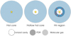 |
Fig. 3 Scheme of the HMC (left), HHMC (middle), and HII region (right) models. The spatio-temporal evolution of the radiation field is included in the computation of the relative abundances only for the HII region models. |
2.2 Physical parameters
The ionized cavity in the HHMC and HII region models is assumed to be filled only with ionized hydrogen and electrons. The temperature is set to the typical HII region temperature of 104 K and the electron density is equal to 105 cm−3. This density is typical of ultracompact HII regions (e.g., Wood & Churchwell 1989). The cavity is present from the beginning of the time evolution and is static in time as we consider a HII region whose expansion is limited by the high accretion flow (Peters et al. 2010a). In order to compute the dust temperature and the radiation field intensity using RADMC-3D we defined the stellar luminosity, the density, the grain properties and the modeling grid.
Stellar luminosity: We considered the model of Hosokawa & Omukai (2009) which predicts the time evolution of a spherically accreting massive proto-star with a constant mass accretion rate of Ṁ = 10−3 M⊙ yr−1. The proto-star is the only heating source of the core, because no external radiation field is included, and its radiation is isotropic. Different to the model presented in Choudhury et al. (2015), the effective temperature Teff of the proto-star is no longer a constant parameter but changes with time as follows:
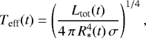 (2)
(2)
where σ is the Stefan-Boltzmann constant, R* is the star radius and Ltot is the total luminosity. The latter parameters are both provided by T. Hosokawa (priv. comm.; see Fig. 4). The time evolution of the stellar parameters covers the range from 54 to 7.8×10⁴ yr. A linear interpolation was used from 0 to 54 yr, assuming that at the beginning all the parameters are set to 0 except for the dust temperature which is set to a constant value of 10 K. Beyond 105 yr, the stellar parameters are constant in time resulting in a constant dust temperature and radiation field intensity.
Density distribution: We considered a Plummer-like density distribution as defined in Eq. 1, with two possible exponents γ (see Fig. 5). In the first case (black lines in the figure), γ is equal to 2.5 like the hot core models in Choudhury et al. (2015). This factor results in a asymptotical radial dependence of the density of r−5, consistent with what is found toward massive dense cores, for example, the dense core Sgr B2(N)-SMA1 that is located close to the UCHII region K2 (Qin et al. 2011). The value rp corresponds to the size of a HII region, while nc is defined so that the density at the ionization front (density of the neutral gas just after the ionized cavity) is 107 cm−3 (or 106 cm−3 for the model with a lower density, see Table 1 for a summary of the different models). In a second case (red lines), γ is equal to 1 which results in an asymptotically radial dependence of r−2. This is similar to the results of Didelon et al. (2015) for the dust density distribution profile found toward the Mon R2 star forming cloud, which contains an embedded UCHII region surrounded by PDRs (e.g., Treviño-Morales et al. 2014, 2016). In this case, rp is fixed and equal to 3×10³ AU whatever the size of the HII region, and nc is equal to 107 cm−3. Thus, when the size of the HII region increases the density at the ionization front decreases. For a HII region of 0.05 pc the density at the ionization front is then 1.56×106 cm−3 and for a HII region of 0.10 pc the density is 4.15×105 cm−3. For simplicity we still annotate the models rXn7p1 (see the abbreviations of the different models in Table 1) despite the fact that the density at the ionization front is 107 cm−3 only for model r0.015n7p1.
Grain properties: We adopted the grains absorption and scattering coefficients from Laor & Draine (1993). The grains are chosen to be 100% carbonaceous, spherical symmetric and with the classical grain size of 0.1 μm (Hasegawa et al. 1992). Despite the fact that RADMC-3D can consider a size distribution and different types of dust grains (e.g., carbonaceous and silicate), the current version of the chemical code Saptarsy considers only one type of grain. This is, however enough to calculate the chemistry because we only need the total grain surface as there is no real radiative transfer treatment.
Modeling grid: RADMC-3D computes the dust temperature and the radiation field intensity in the entire modeling grid and for each time step given by the time evolution of the stellar luminosity. We used a 3D spherical grid. The edges of the modeling grid are reached when the density has decreased to 10 cm−3. The size of the grid is a parameter that can vary, for example, to filter out the extended emission by decreasing the size of the grid.
In summary, the HII region and the HHMC models have the same structure: same temperature, same opacity and a cavity of ionized hydrogen with no dust. The difference between these two models is the UV radiation field which is accounted for in the case of the HII region models, but is not included in the HHMC model, during the computation of abundances performed by Saptarsy. For the HMC model, the density near the star is high enough to completely attenuate the UV radiation.
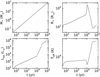 |
Fig. 4 Time evolution of the parameters for an accreting massive proto-star with an accretion rate of 10−3 M⊙ s−1 (Hosokawa & Omukai 2009). The different panels show the mass of the star M* (top left), the star radius R* (top right), the total luminosity Ltot (bottom left) and the effective temperature Teff (bottom right). |
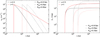 |
Fig. 5 Left panel: density distributions as a function of radius for a Plummer function with exponent γ = 2.5 (black) and γ = 1 (red) for the three sizes of HII regions: 0.015 (solid), 0.05 (dashed), 0.10 pc (dash-dotted). Right panel: visual extinction as a function of radius. |
Model abbreviations.
2.3 Chemical code
Saptarsy (Choudhury et al. 2015) is a gas-grain code based on the rate equation approach solving both the spatial and temporal evolution of chemical abundances. It uses the Netlib library solver DVODPK5 to solve the ordinary differential equations and the MA28 solver6 for sparse systems of linear equations from the Harwell Mathematical Software Library.
We extended the use of the code presented in Choudhury et al. (2015) to study HC/UCHII regions and their associated internal PDRs. To do this, we included the spatio-temporal evolution of the local radiation field intensity G(r,t) in Draine unit (Draine 1978), which is obtained using the mean intensity of the radiation field Jλ (r) computed by RADMC-3D for several time steps given by the time evolution of the stellar parameters. The computation of Jλ (r) accounts forthe attenuation by dust once the UV radiation penetrates the PDR.
 (3)
(3)
In this work we have used a chemical network, containing 183 species, based on a reduced version of the OSU network (Garrod 2008), including new reactions for HCN and HNC (Graninger et al. 2014; Loison et al. 2014). The reduced version of the OSU network speeds up the computational time, and excludes species not relevant for the current work, such as those species bearing Cl, P, Na, and Mg, as well as all anions and long carbon chains with more than four carbon atoms. For Si and Fe, only the neutral, ionized, and grain surface atomic form were included in the network. In addition, the desorption energies ED of different species have been updated, and the values used can be found in Table 2. Since measurements of diffusion barriers Eb only exist for a few species, we considered them to be related to the desorption energy as Eb ∕ED = 0.50 (Vasyunin & Herbst 2013).
Photon processes and secondary photon processes were not used in the previous version of Saptarsy (Choudhury et al. 2015). For the present work, we have added photo-dissociation reactions in the gas phase and on the grain surface as described in Semenov et al. (2010). Photo-desorption is also included for 11 species7 (s-H, s-H2, s-O, s-O2, s-OH, s-H2O, s-CO, s-HCO, s-H2CO, s-N2, and s-CO2) as defined in Le Bourlot et al. (2012) in the case of H2. In the associated reaction rate the photon flux also takes into account the secondary photon flux. The direct dissociation by cosmic-rays and the secondary photon processes were treated the same way in the first version of Saptarsy. Secondary photon processes are now treated as expressed in Le Petit et al. (2006). Desorption via exothermic surface reactions, also called reactive desorption, with an efficiency of 1% has been added following Garrod et al. (2007). Furthermore, self-shielding is an important process in internal PDRs. We included a simple treatment of the self-shielding for H2 and CO following Lee et al. (1996) (see also Draine & Bertoldi 1996 and Sternberg et al. 2014 for H2 and Panoglou et al. 2012 for CO), which is used in the HII region models. Appendix A describes other modifications done in the chemical code Saptarsy.
The initial abundances, noted ini1 (see Table 1 for the abbreviations), are obtained by simulating the collapse of aprestellar core in two steps. We started with the elemental abundances from Wakelam & Herbst (2008), a core with a temperature of 10 K, an extinction of 10 mag and no radiation field. In the first step, the core has a density of 104 cm−3 and we let the chemistry evolve up to 105 yr. We then increased the density to 107 cm−3 to simulate the density increase during the process of collapse, and repeated the process using the results of the first step. This means that for all the models (HMC, HHMC, and HII region), we started with a medium where molecules are depleted onto grains except for hydrogen which is found in its molecular form H2. The carbon is mostly found in s-CO, the oxygen is in s-H2O, and the nitrogen is mainly in s-N2 as seen in the second column of Table 3. We note that carbon is also found in s-CH4 and s-HCN, oxygen in s-O and s-OH and nitrogen in s-HNO and s-NH3. In order to simplify the comparison between models, we used the same initial abundances, except for models that have the second set of initial abundances ini2 (see Col. 3 of Table 3). This second set of initial abundances ini2 is obtained for the steady state of a prestellar core model at a density of 107 cm−3. In these conditions the species are also frozen on grains, except hydrogen which is in its molecular form in the gas phase. Carbon is found mostly in s-CH4, oxygen in s-H2O, and nitrogen in s-NH3.
Desorption energies.
Initial abundances of the principal species used in the models are shown in the second and third columns.
3 Results and analysis
3.1 Models
In the following we present the parameters used for the different models considered. Our reference model is an HII region with a size of 0.05 pc (r0.05), a density of 107 cm−3 at the ionization front (n7) and a Plummer exponent of 2.5 (p2.5). The model uses the first set of initial abundances (ini1), a chemical network with 183 species (s183) and a cut-off density of 101 cm−3 (c1). The size and density of the HII region is consistent with the values commonly found for HC and UCHII regions (see Kurtz 2005). In addition to this model, we have changed different parameters to see their effects on the chemistry. The different models are:
we consider first the reference model of HII region and the associated HHMC and HMC models;
models with different sizes of HII regions are produced. In addition to RHII = 0.05 pc (10300 AU) we used RHII = 0.015 pc and 0.10 pc (or 3000 and 20600 AU). The model where RHII = 0.015 pc corresponds to a HCHII region, while the one of 0.10 pc is at the transition from a UC to a compact HII region (Kurtz 2005; Sánchez-Monge et al. 2013a). In Appendix B.2 we present the results obtainedfor the same models but with a different density profile where the exponent of the Plummer-like function (Eq. (1)) is set to 1;
-
we also considered models with a lower density at the ionization front: 106 cm−3. This value is typically found in the dense gas surrounding UCHII regions;
in addition to the initial abundances ini1, we also considered a second set of initial conditions – ini2. These initial conditions are shown in the second column of Table 3;
finally, we considered a model for which the modeling grid is stopped at a higher cut-off density of 106 cm−3 (instead of 10 cm−3). This results in a smaller grid that contains only the emission from the inner core, and therefore excludes the extended and more diffuse envelope;
additional models are presented in Appendix B.2 where we set the exponent of the Plummer-like function to 1 (model p1) and B.1 where we used a chemical network with 334 species (model s334).
To distinguish between the different models we use the abbreviations presented in Table 1 and the different comparison points are referred as “Item i” from the list of Sect. 3.1. We annotate the reference model as mHII:r0.05n7ini1c1p2.5s183 and unless indicated otherwise, all parameters are considered to be set to their reference values in the different models. In the following, we discuss how the temperature, density structure, abundances and line intensities change from model to model.
3.2 Temperature and radiation field variations
The spatio-temporal evolution of the dust temperature and the radiation field intensity for the reference model mHII:r0.05n7ini1c1p2.5s183 are presented in Fig. 6. The variation of these two parameters can be used to determine different chemical transitions during the core evolution. We started with the initial conditions (Td = 10 K and G = 10−20 Draine unit) for the first 50 yr, which correspond to the grain surface region where all the molecules are frozen onto the grain surface. After this time, G is equal to 10−1 and Td is higher than 50 K. We enter into a molecular region as the species are released into the gas phase. Deeper in the cloud the transition from grain surface to gas phase might be delayed because the temperature is still too low. From approximately 104 yr, the radiation field strength increases but only for extinctions up to 10–20 mag. The temperature is also the highest in this region. It is an atomic-ionized region, i.e., a PDR, although the spatial resolution and the approximate treatment of ionization and thermal balance induce some inaccuracies that disappear further in. For the latest phase of the evolution (after 104 yr) and deep in the cloud (AV > 20 mag), the temperature is the only parameter influencing the chemistry due to absence of the radiation field. The temperature is high enough, ~100 K, to ensure that all molecules are in the gas phase.
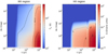 |
Fig. 6 Spatio-temporal evolution of the dust temperature (left) and radiation field intensity (right) in the case of the reference model mHII:r0.05n7ini1c1p2.5s183. Contours are plotted: solid line for Td (30, 100 and 200 K) and dashed lines for G (10−1, 103 and 106 Draine unit). |
3.3 Abundances
In this section we present the spatio-temporal profiles of the abundances, relative to n(H), obtained for the different models detailed in Sect. 3.1. We obtained these abundances with Saptarsy for all species present in the chemical network. We focus principally on a few species such as HCN, HNC, water and some others that are more relevant in HMCs including methanol and in HC/UCHII regions like ionized and atomic species.
3.3.1 Item 1 – HMC/HHMC/HII region
In Fig. 7 we compare the abundance of HCN for the HHMC and HMC models with the following parameters r0.05n7ini1c1p2.5s183. To help for the comparison and because the extinctions are differentfor both models the abundances are shown as a function of the density in y-axis, from 107 to 104 cm−3 for the HHMCmodel and from 5.6 × 107 cm−3 for the HMC model which does not have the ionized cavity around the proto-star. We notice that the 100 K temperature at late times is reached at a density higher than 3 × 106 cm−3 for the HHMC model whereas it occurs for a lower density in the HMC model. The 150 K temperatureis reached for slightly higher densities in the HMC model. However, we see that from 107 to 104 cm−3 the abundances and their spatio-temporal evolution are consistent in both models. The same is found for the other species of the chemical network.
We also compare the distribution for the HII region model and the HHMC model to investigate the differences in the abundances when a UV radiation field intensity is added to the model. Figure 8 shows the abundance profile of HCN and C+ for the reference HII region model mHII:r0.05n7ini1c1p2.5s183 (left panels) and for the one of the HHMC model mHHMC:r0.05n7ini1c1p2.5s183 (right). We choose these two species because they present the two different behaviors happening in presence of a radiation field. The well known PDR tracer C+ is formed by photo-dissociation and photo-ionization in regions where the radiation field is strong. On the contrary, HCN is a more fragile molecule against UV radiation and therefore more easily destroyed (Fuente et al. 1993). However, HCN can also be found in these high temperature and dense environments (Paglione et al. 1995, 1997), particularly in highly excited energy states (Ziurys & Turner 1986).
The ion C+ is formed in the HII region model, at ~100 yr when the UV radiation becomes strong (see dashed contours), while HCN disappears. From the comparison of these abundance profiles, and considering other species, we identified the grain-surface chemistry region, as well as the molecular gas and the atomic-ionized gas regions indicated previously in Sect. 3.2. In addition, a region partly molecular partly atomic can be seen as well as a transition region between this molecular-atomic region and the molecular region. Schemes of the different regions seen in the HII region and the HMC/HHMC models are shown in Fig. 9. The molecular-atomic and atomic-ionized regions constitute the internal PDR in the HII region models. It is created by the UV radiation field. In the HMC/HHMC models, the grain surface chemistry region can be larger close to the edge of the cavity depending on the considered species (see the right panel of Fig. 9). For instance, in the case of methanol, thermal desorption occurs before 100 yr in model mHII whereas it starts at around 104 yr in models mHMC and mHHMC. This is not the case for species with low desorption energy such as CO. For those molecules desorption happens at the same time as in the HII region models, but with a smoother transition.
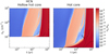 |
Fig. 7 Spatio-temporal evolution of the abundance of HCN for the model mHHMC:r0.05n7ini1c1p2.5s183 (left panels) and the corresponding model mHMC (right). Contours are plotted in solid line for Td (30, 100 and 200 K). |
3.3.2 Item 2 – Size of the ionized cavity
The size of the ionized cavity affects the duration of the grain surface chemistry. Models with larger HII region cavities have a grain surface chemistry region (as shown in Fig. 9) that extends deeper into the core, stopping at 100 yr for the mHII:r0.015 and lasting until 104 yr for mHII:r0.10 (see the high extinctions of the abundance profile of HCN in top panels of Fig. C.1). s-H2O seems to stay on the grain surface even after 105 yr when the size of the cavity increases. This is because the temperature increases more slowly in the core due to the distance from the star.
In the molecular-atomic region, the abundance of most gas phase species becomes larger as the core evolves for models with larger ionized cavities models because of the smaller radiation field reaching the gas surface. This is also the case for grain surface species with high desorption energies such as methanol. The desorption of more complex molecules like methanol is delayed when we increase the size of the cavity. In addition, the size of the atomic-ionized region is independent of the temperature and only depends on G.
Furthermore, when AV > 10 mag and between 103 and 104 yr, we see a decrease in the abundance of HCN, as well as HNC and CH3OH, before a sudden increase of the abundances due to thermal desorption (Fig. 8 and top panels of Fig. C.1). This decrease, mainly due to a significant accretion of the species on the grain, appears closer to the ionization front when the size of the HII region increases.
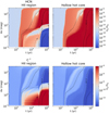 |
Fig. 8 Spatio-temporal evolution of the abundance of HCN (top panels) and C+ (bottom) for the reference model mHII (left panels) and model mHHMC (right). Contours are plotted: solid line for Td (30, 100 and 200 K) and dashed lines for G (10−1 and 103 Draine unit). |
3.3.3 Item 3 – Density at the ionization front
The density at the ionization front is another parameter that affects the chemistry. The abundance of a few ions such as N+, NH+ and O+ is higher for models with lower density during the entire evolution, especially in the atomic-ionized region. For a lower density and at the beginning of the evolution, the abundances of He+ is larger and therefore it reacts to form more of these ions. The higher abundances of these ions are maintained throughout the evolution. From 100 to 104 yr and for extinctions up to 2–3 mag, the abundance of C+ and O are also higher for the model with a lower density, hence the abundance of gas phase molecules, such as HCN, NO, or NH, as well as grain species is lower (see Fig. C.2).
3.3.4 Item 4 – Initial abundances
Using different initial abundances leaves the dust temperature and radiation field intensity profiles unchanged. In Fig. 10 we show the abundances of C4H2 and NH3 for model ini1 (left panel) and ini2 (right). In model ini2 we start with about 15 times more s-CH4 and about ten times less s-CO as shown in Table 3. The evolution starts with less complex molecules, their precursors and carbon chains in the gas phase and on grain surfaces in model ini2. Above a dust temperatureof 30 K carbon chains form on the grain surface until they desorb at a temperature of about 100 K. In the gas phase, they begin to form only above 20 K instead of 15 K for model ini1 (see the case of C4H2 in the top panels of Fig. 10). Therefore, in model ini2, up to three orders of magnitude more carbon chains are produced, for a longer period that lasts about 2–3 × 10⁶ yr longer (see also the warm carbon-chains chemistry (WCCC) model in Sakai et al. (2009) for further discussions).
In the molecular region (cf. Fig. 9), from 104 to 106 yr, the abundance of CH4, H2 O and NH3 is higher in model ini2, 15, 5, and 10 times higher respectively (see the case of NH3 in the bottom panels of Fig. 10). The abundance of radicals leading to these species is also higher but in a lesser extent. For instance the abundances of CH and OH are 10 and 3 times, respectively, higher for model ini2. On the contrary, CO, O2 and N2 are less abundant, approximatively 10, 7, and 25times less, up to 106 yr when they become the dominant species. Additional results are presented in Appendix B.3.
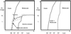 |
Fig. 9 Schematics showing the different regions in the HII region models (left) and in the HMC/HHMC models (right). |
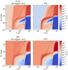 |
Fig. 10 Spatio-temporal evolution of the abundance of C4H2 and NH3 for the reference model mHII:ini1 (left panel) and model mHII:ini2 (right panel). Contours are plotted: solid line for Td (20, 30, 100 and 150 K) and dashed lines for G (10−1 and 103 Draine unit). |
3.3.5 Item 5 – Cut-off density
When changing the cut-off density in the model from 10 cm−3 (c1) to 106 cm−3 (c6), the abundance profiles remain the same. The only difference is that they do not extend as deep into the envelope for c6 because the grid is cut out at a higher density and so at a much closer radius from the star.
3.4 Dissociation front
We used the abundance profiles to study the dissociation front and the size of the PDR. In Table 4 we present the position of the dissociation front located where  = 0.1. In all the cases the width of the PDR (Δ rPDR) is extremely small, about tow orders of magnitude, compared to the size of the HII region. This results in the PDR being a very thin shell surrounding the HII region. For models mHII:p2.5 the size of the PDR decreases when the size of the HII region increases, and the density at the dissociation front is higher, because the radiation field is less strong at the ionization front. On the contraryand as we could expect, the size of the PDR increases when the density at the ionization front decreases because the UV radiation can penetrate deeper into the core. For the models mHII:p1 the distance between the ionization front and the dissociation front increases with the size of the HII region despite the lower incident radiation field due to a decrease in density at the ionization front.
We notice here that the H/H2 transition occurs for higher visual extinction (>5 mag) compared to typical PDRs where it happens at AV < 2 mag. This is due to the extremely strong radiation field in the models and also to the limited spatial resolution that could underestimate the H2 self-shielding. For example, it is about two orders of magnitude higher than what can found in the Orion bar. For models with lower incident radiation field the H/H2 happens for lower extinction, for example, if we divide the radiation field intensity by ten in the reference model the dissociation front is located at ≈3.9 mag. If divided by 100 it is at 2.6 mag.
H2 dissociation front position from the ionization front at 105 yr for the different models.
3.5 Line emission
We studied the line emission for the molecular and atomic transitions presented in Table 5. We have selected species such as C+ and O that can be produced in the internal PDR due to the UV radiation field, and other species such as HCN and CH3OH that can be either destroyed or not formed. We also study vibrationally excited HCN and HNC as they trace mainly hot gas found close to the HII regions (Rolffs et al. 2010). Most of the transitions are chosen because the lines are optically thin and unblended by other lines from the same species. Thus, we used HC15N and HN13C instead of HCN and HNC8. No isotopologues are included in the chemical network, so to obtain their spectra we used the local ISM isotopologue ratios from Wilson & Rood (1994): 12C/13C = 70, 14N/15N = 450 and 16 O/18O = 500.
We used RADMC-3D (see Sect. 2) to produce synthetic cubes from which we can extract synthetic maps and spectra for the different models listed in Table 1. In the following, we describe the results obtained for each of them.
List of selected species, one of their transition and the corresponding frequency in GHz.
3.5.1 Item 1 – HMC/HHMC/HII region
In Fig. 11 we show the maps of the peak intensity of HC15N (1–0) for the reference model mHII:r0.05n7ini1c1p2.5s183 (top panels) and model mHMC:r0.05n7ini1c1p2.5s183 (bottom). The maps are shown for different times between 103 and 105 yr and the x-axis represents the distance in parsec from the proto-star. The top six maps have the original resolution of the model of 0.5 ″ for an object located at 1 kpc (corresponds to a pixel size of 500 AU), while the six bottom panels showthe spectra convolved to the beam of the IRAM 30 m telescope at the frequency of HC15N (1–0), which corresponds to 29.22″. The maps for the HHMC model are not shown in Fig. 11 because the results are very similar to the HII region maps for these three particular time steps. We see that the emission of HC15N increases with time and is weaker for the HII region compared to the HMC model. It also presents a ring structure around the central proto-star. This ring structure is not seen in the convolved maps9.
Synthetic spectra obtained for CH3OH, centered at337.6 GHz, are shown at 1.5×10⁴ and 7.5×10⁴ yr in Fig. 12 for model mHII (black), mHHMC (blue) and mHMC (green). Contrary to the maps presented in Fig. 11, these spectra (as well as all the others used in this work) have a pixel size of 100 AU (0.1″ for an object at 1 kpc) and are not convolved to the beam of any observations. For the HHMC and HII region models there is no methanol emission at about 104 yr. Later, the emission of these two models increases but still remains weaker by almost one order of magnitude compared to the HMC model. After that time, both the HHMC and HII region models have similar integrated intensities for these species. This high difference between the HMC model and the two others is due to the much higher column density in the HMC model as there is no cavity.
The temporal evolution of integrated intensities for all the species and their transitions listed in Table 5 is shown in Fig. 13. The emission of HN13C is similar to the ones of HC15N. Until 104 yr, the emissionof the HHMC model is also stronger than the emission in the HII region model by approximately one order of magnitude for HC15N and a bit less for HN13C. After that time, both models have similar integrated intensities for most of the species. The emission increases in time for all models as the species are released from the dust grains and then formed in the gas phase. The presence of the cavity has a strong effect on the intensities of the HHMC model which are in general lower than the intensities of the HMC model due to a smaller column density. On the contrary, the emission for C+ is stronger in the HII region model and appears to be undetectable for the HMC and HHMC models with an integrated intensity lower than 4 × 10⁻⁴ K km s−1.
In order to determine if the lines are detectable with current astronomical facilities, we assumed an arbitrary detectability threshold for all lines derived from observations with the IRAM 30 m telescope10. Considering a minimum value of the rms noise of about 3 mK (Treviño-Morales et al. 2014, 2016) in the 3 mm wavelength range where most of the selected lines are located, all lines with a peak intensity lower than 15 mK or with an integrated intensity below 5 × 10⁻² K km s−1 (with an assumed line width of 5 km s−1) can be considered undetectable.
There is no general trend in the evolution of the integrated intensities from one species to another. The emission of oxygen in the different models behaves like the emission of C+. For C, the HII region emission is stronger than the two other models but it becomes equal to the HHMC emission at 104 yr and the HMC emission is stronger than the HHMC emission up to 104 yr before it decreases to become undetectable. For HCO+ and N2 H+, the HHMC and HII region emissions are equal. For H2 CO, H O, and NH3, the HII region emission is stronger than the HHMC emission up to 104 yr. And then it is slightly weaker until 4×10⁴ yr for H
 O and NH3 before they become equal. For CH3OH, HCO, and CN the behavior is the same as HN13C but the HMC emission becomes stronger again after 2 × 10⁴ yr in the case of CN. In the case of the vibrationally excited state of the transition 7–6 of HCN and HCN, the HHMC emission is stronger than the HII region but only until 3×10⁴ yr for HNC.
We also note that the emission of some species is considered undetectable because the integrated line intensity is below the detectability threshold of 5×10⁻² K km s−1. This is the case for H O and NH3 in the HHMC and HII region models before 104 yr. The vibrationally excited lines of HCN and HNC are undetectable before about 3×10³ yr for the HHMC model and until 104 yr for the HII region model. CN can be considered undetectable before 103 yr for the HMC and HHMC models. The HMC emission for C is lower than the threshold after 2 × 10⁴ yr. In the case of CH3OH, the line is undetectable between 104 and 2×10⁴ yr approximately for the HII region model.
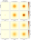 |
Fig. 11 Time evolution of the HC15N (1–0) maps for the reference model mHII (top) and the associated model mHMC (bottom). The y-axis is the same as the x-axis. The bottom maps represent the same spectra convolved to the beam of the IRAM 30 m telescope. The convolved spectra have a weaker intensity. |
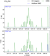 |
Fig. 12 Example of the time evolution of CH3OH spectra around 337.6 GHz for the reference model mHII (black) and the associated model mHHMC (blue) and mHMC (green). Top: t = 1.5×10⁴ yr. Bottom: t = 7.46×10⁴ yr. |
 |
Fig. 13 Time evolution of the integrated intensities of all the species presented in Table 5. Model mHII is represented in black, model mHHMC in blue and model mHMC in green. The red dashed line represents the detectability threshold of 5 × 10⁻² K km s−1 obtained with an assumed rms noise of 3 mK. |
3.5.2 Item 2 – Size of the ionized cavity
We also investigated the variation of the integrated intensities when changing the size of the ionized cavity. In the top panel of Fig. 14 we summarize the main behavior of the integrated intensities for the selected species. The detailed time evolution of the integrated intensities are shown in Fig. C.3.
The species C+ and O are brighter for smaller HII regions. The opposite is true for N2 H+. For the other species the integrated intensity is larger for the smallest HII region at the beginning of the time evolution and for the biggest HII region at the end of the evolution. Species desorb earlier in models with a smaller ionized cavity. Later they are abundant inthe three models, but the column density is higher in models with a bigger cavity, thus the intensity is stronger.
In the cases of HC15N, HN13C, H2 CO, and CH3OH the integrated intensity slightly decreases due to decrease of the abundances mentioned in Sect. 3.3.2. Then it increases with a delay when the size of the HII region increases. This is due to the delay of the desorption of grain species. The results found for a density profile where γ = 1 (model p1) are presented in Appendix. B.2 but are also summarized in the top panel of Fig. 14.
3.5.3 Item 3 – Density at the ionization front
The variation of the density also influences the integrated intensities (see second panel of Figs. 14 and C.4). Therefore, the emission of mHHMC at this density is always stronger except before 500 yr. For the other density models n7 and n6, the emission of all species is stronger for the model n7 except for C+ and O as well as for H2CO until 104 yr.
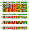 |
Fig. 14 Schematic summarizing the results of the time evolution of the integrated intensities for the different models: size of the ionized cavity and density profile (top panel), density at the ionization front (second panel), initial abidances (third panel) and cut-off density (bottom panel). Lines with the integrated intensity Iint > 100 are represented in green, 10 < Iint < 100 in yellow, 1 < Iint < 10 in orange and Iint < 1 K km s−1 in red. Undetected lines, with integrated intensities lower than the detectability threshold of 5 × 10⁻² K km s−1, are represented in gray. |
3.5.4 Item 4 – Initial abundances
When we compare models with different initial abundances (see third panel of Figs. 14 and C.5), we obtain different results except for C+ and O. The integrated intensities are also very similar for molecules like H O and HCO+ and C. The largest difference occurs for N2 H+ for which model ini2 gives integrated intensities that are more than two orders of magnitude lower. This is due to the fact that there is a difference of about five orders of magnitude in the initial abundance of N2 H+. This difference is one of the largest and is due to the destruction of N2 H+ and other N-bearing species to form NH3 after 109 yr in the prestellar core model ini2. We also obtain lower intensities for HN13C, HC15N as well as for HCO and CN up to about 104 yr.
3.5.5 Item 5 – Cut-off density
When comparing the integrated intensities for models with different sizes of the modeling grid c1 and c6 (see bottom panel of Figs. 14 and C.6), we observe that C, HCO, HCO+, CN, and N2 H+ integrated intensities are lower in model c6, about ten times lower after 104 yr suggesting that the emission of these species is important in the outer region of the model. The methanol and formaldehyde emission is slightly affected. It is less than a factor of two lower for model c6, between 103 and 104 yr approximately for the first molecule and between 104 and 3×10⁴ yr for the second one suggesting that the emission of these species is mainly coming from the inner core.
4 Discussion
From the abundance profiles of the HII region and HMC/HHMC models we have defined different regions depicted in Fig 9. The evolution starts with molecules frozen onto the grains surface, the grain surface chemistry region (cf. Fig.9). It ends when the proto-star is evolved enough to emit IR as well as UV photons in the HII region model. Then, as the proto-star is switched on, the temperature and radiation field increase. The IR photons penetrate deeper into the cloud and heat up the grains leading to the evaporation of some grain surface species between 15 and 30 K for high extinctions but it takes more time than close to the HII region. Molecules with high desorption energy thermally desorb later. We note that the inclusion of photo-desorption reactions may accelerate the desorption of some species. The molecular-atomic and atomic-ionized regions - the internal PDR - is created by the radiation field which dissociates and ionizes the species. This formation ofthe PDR is the main difference between the HII region and HMC/HHMC models. In addition, the decrease in the effective temperature of the proto-star (see bottom right panel of Fig. 4) happening at 104 yr affects the temperature and radiation field intensity. They both decrease at this time and thus affect the abundance and line emission of the species.
We haveseen that C+ and O emit only in the HII region models and their emission is not affected when we remove the envelope. This indicates that they are possible tracers of the internal PDR. Furthermore, we have seen that the internal PDR is extremely thin with a size ranging between 50 and 1500 AU depending on the model parameters. Assuming a source at a distance of 1 kpc, we would need an angular resolution of maximum 0.04–0.05″ to be able to resolve the minimal size of the internal PDR. Thus, to trace it and avoid extended emission we need the high spatial resolution interferometric observations which are now possible with ALMA. However, there are no instruments to conduct the observations in the THz frequency regime that are necessary to resolve the C+ and O emission associated with the internal PDRs. In addition, limitations of the models, such as the absence of an external radiation field, might cause the underestimation of the emission of these atoms coming from the envelope. Interferometric observations are thus absolutely mandatory to filter out the extended emission from the envelope.
The emission from the envelope affects the emission of some species. C could also trace the internal PDR as the emission is stronger in the HII region in the early stage of the evolution until 104 yr. This is more difficult to observe due to the short time spent by the object in this phase. In addition, C emission is affected by the envelope mostly after that time as the HMC emission is in absorption and the intensity of the line in the HII region model decreases when we filter out the extended emission in the late times of the evolution. Since atomic carbon can be observed with ALMA band 8, this is an interesting test to try. For the species N2 H+, HCO, HCO+, and CN, the emission is also strongly affected by the envelope. Due to the decrease in their emission they might not be good tracers to distinguish between HII regions and HMC as they do not trace the inner core. NH3 emission is also affected when removing the extended emission but in a lesser extent.
Molecules like CH3OH, H O or NH3 appear to be detectable (Ipeak ≥ 15 mK) around 104 yr for the HHMC models and only around 4×10⁴ yr for the HII region models. The intensities of methanol in the HHMC models yet remain quite low (Ipeak ~ 0.1 K) during the time when the HII region emission is still too weak. These molecules are likely destroyed mainly during the desorption process when the UV radiation field increases. The few molecules that desorb are photo-dissociated in a short time (~50 yr). They appear again after 104 yr due to thermal desorption outside the PDR before being destroyed at 106 yr. However in the HMC model, i.e., the model without the ionized cavity around the proto-star, the abundance of these molecules is high at the center inducing high column densities and strong intensities from 100 yr, compared to the HHMC model and thus the HII region model. These molecules might help in tracing the HMC phase. Similarly, H2 CO is always detectable for the three models but the emission for the HMC model is much stronger despite that they tend to be equal once it thermally desorbs. In addition, a ring structure seems to appear in the HII region model in the raw synthetic maps. But the convolution to the beam of the IRAM 30 m telescope for example attenuates this effect. The vibrationally excited levels of HCN trace the hot gas and could be used to distinguish the hot core and the HII region as the emission is stronger in the HHMC model. This is not the case for vibrationally excited HNC. This difference between HCN and HNC could happen because the abundance of HCN is high near the ionized cavity (≥10−6) for the HHMC model whereas the HNC abundance is about four magnitudes lower. The region up to an extinction of 5 mag has then more influence on the intensity for HCN.
Our results show that the region where UV radiation influences chemistry is spread in time but remains thin, mainly for high density (≥106 cm−3). Hence, we do not obtain certain molecules which appear to be abundant in observations. HCO+ is usually optically thick in observations of hot cores or HII regions but in our models it is destroyed around 104 yr. Destruction of HCO+ is mainly due to dissociative recombination forming H and CO and by reactions with HCN and H2 O which are really abundant because of thermal desorption. In addition, CO+ is an important species in PDRs and its abundance is enhanced when irradiated by strong UV fields (e.g., Treviño-Morales et al. 2016). However we do not produce enough CO+ in the models compared toobservations. CO+ is rapidly destroyed to form C+. The medium is too dense and the UV radiation cannot penetrate deep enough into the cloud and thus the PDR remains too thin. This issue has been discussed in Bruderer et al. (2009b). They circumvent it by modeling a proto-star embedded in a cavity produced by a bipolar outflow. It provides a larger surface to the UV radiation.
There is also an important dependence of the results on the initial abundances. Obtaining good initial conditions is thus critical. In this work, the first set of initial abundances, from the collapsing cold core in two steps, seems to be more realistic than the second set. However, implementing a real collapse of the core by adding the temporal evolution of the density (similar to Garrod & Herbst 2006) would be the next step.
The spectra are obtained without including the free-free emission which might be an important physical parameter for transitions at lower frequencies in the HII region models. In our models, the continuum level for the HII region models’ spectra is low (close to zero) for the lower frequencies, while HII regions may be bright up to 100–200 GHz. Another aspect that might influence the emission of the species is the position from which the synthetic spectra is obtained. In this work, all synthetic spectra used to compute the integrated intensities are chosen at the center of the synthetic maps, where the proto-star is located, in order to probe the gas in the entire region. Choosing spectra located at the position of the internal PDR could induce different variations for the HII region models compared to the HHMC models.
4.1 [HNC]/[HCN]
In Fig. 15 we present the spatio-temporal variations of the abundance ratio [HN13C]/[HC15N] and [HNC]/[HCN] for the HII region (left) and HHMC (right) models. The colorbar varies from 10−3 and 14 because the ratio varies from approximately 10−2 to 14, if we do not consider the PDR region from 104 yr and AV < 5 mag. The maximum ratio appears in the HII region model. In the HHMC model the maximum is around 6.5. The variations for the ratio [HNC]/[HCN] are from 10−3 to 1.07 for mHHMC and to 2.16 for mHII. The variations in the abundance ratio result into temporal variations of the line intensity ratio seen in Fig. 16. The main contribution to the intensity ratio comes from the part of the core where the extinction is higher than 4 mag approximately, whatever the size of the HII region. The ratio is barely affected by the evolution of the radiation field which influences the core only for extinctions lower than 5 mag. Different works on the [HNC] to [HCN] ratio show that it depends on the kinetic temperature in the cloud (Goldsmith et al. 1986; Schilke et al. 1992; Wang et al. 2009; Jin et al. 2015). In the model this ratio increases until the temperatureis around 20 K, then it decreases. It goes through a minimum when the temperature of the core is between 40 and 50 K. The ratio increases again until the temperature reaches about 150 K. The behavior found for [HN13C]/[HC15N] is the same for [HNC]/[HCN]. This strong decrease around 40 K is due to the thermal desorption of s-HCN which is faster than for s-HNC. The thermal desorption of s-HNC is slowed down due to the decrease of the abundance of s-HNC around 3×10³ yr because it reacted with s-H to form s-HCN or HCN via reactive desorption.
In Schilke et al. (1992) the minimum [HNC]/[HCN] for a cloud with a density of 107 cm−3 appears at 30 K and in Graninger et al. (2014) the abundance ratio is found to go through a minimum for a temperature around 30–40 K. This ratio also depends on the density of the core as the integrated intensity ratio is smaller for lower density due to a lower abundance ratio but the minimum is the same.
The intensity ratio of the vibrationally excited line of HNC and HCN decreases from 104 to 105 yr. Before thesetimes the ratio is unrealistic because the line emission is extremely low or undetectable. The decrease of the ratio indicates that the major contribution to the line emission for these transitions comes from the inner core where the temperature is high. The abundance ratio decreases close to the ionized cavity for mHII and mHHMC affecting in a similar manner the intensity ratio.
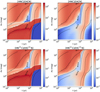 |
Fig. 15 Spatio-temporal evolution, focused between 100 and 105 yr, of the abundance ratio [HNC]/[HCN] for the reference model mHII (left) and the corresponding mHHMC model (right). Contours are plotted for Td (20, 30, 40, 50, 100 and 150 K). The bottom panels show the same results for [HN13 C]/[HC15N]. |
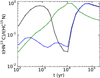 |
Fig. 16 Time evolution for the reference model mHII (black), mHHMC (blue) and mHMC (green) of integrated intensity ratio (HN13C (1–0)/HC15N (1–0)) |
4.2 Gas temperature in the PDR
For all the models presented here we have assumed that the gas temperature is equal to the dust temperature. We know that this is not the case in the internal PDR where the gas temperature is usually approximately one order of magnitude higher than the dust temperature. We know that some species not investigated in this paper such as mid and high-J transitions of CO may be strongly affected by a gas temperature of a thousands Kelvin and trace the hot gas and thus the internal PDR (e.g., Lee et al. 2015). But for the species and transitions investigated in this paper the assumption Tg = Td seems to be fine. We have produced one model of a core with an embedded HII region similar to the reference model but where the gas temperature is increased for the abundances’ computation with Saptarsy (model mHII-Tg). The gas temperature is defined as follows:
 (4)
(4)
where β = 20 and α = 1.5. This equation is obtained from a fit of a model, with physical conditions close to our HII region model, produced by the Meudon PDR code (Le Petit et al. 2006).
In Fig. 17 we show the time evolution of the integrated intensities for model mHII (black), mHHMC (blue), mHMC (green) and model mHII-Tg (red), for HC15N, C+, C and NH3. Apart from HC15N these are the species the most affected by the increase of the gas temperature. C+ and NH3 present different behaviors from the reference HII region model only before 3000 yr. Objects of this age do not yet present an internal PDR as it appears at around 104 yr in the models and it seems unlikely that we would observe such young objects. Atomic carbon is then the species of most concern here because its intensity is lower than a model assuming Tg = Td all along the time evolution.
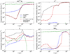 |
Fig. 17 Time evolution of the integrated intensities of HC15N, C+, C and NH3 (see the corresponding transition in Table 5). The reference model mHII is represented in black, model mHHMC in blue and model mHMC in green and the new HII region model in red. The red dashed line represents the detectability threshold of 5×10⁻² K km s−1 obtained with an assumed rms noise of 3 mK. |
5 Conclusion
5.1 Summary
We investigated the spatio-temporal evolution of the chemistry in HC/UCHII regions and hot molecular cores using the spatio-temporal evolution of the dust temperature and the UV radiation field. this is done in order to obtain the detailed modeling of relative abundances and the temporal evolution of line emission of selected species.
All the abundance profiles clearly show a difference between these two evolutionary stages of massive star formation. But the typical tracers of the HC/UCHII region phases, C+ and O, appear to be unobservable due to the capabilities of the current instruments which do not allow to resolve the internal PDR in the THz range, although atomic carbon might be a good tracer to be observed with ALMA. We find the internal PDR to be extremely thin, with a size ranging from about 50 to 1500 AU. This barely affects the emission of the other species. TheHMC emission is stronger than the HII region during most of the time evolution for some species: HC15N, HN13C, H2 CO, H O, NH3, and CH3OH. This is due to the increased column density. More species could exhibit this behavior and remain to be investigated.
5.2 Outlook
In addition, the models can be improved as indicated below:
we would also like to investigate HC/UCHII regions in the context of ionized cavities (Peters et al. 2010a) or PDRs on outflow cavities (Visser et al. 2012; Bruderer et al. 2009b) which create large surfaces and thus more easily observable chemistry. Therefore, we would have to increase the complexity of the source structure;
we are currently improving the treatment of the grain chemistry by incorporating a multilayer ice mantle;
finally, we plan to implement the treatment of dynamics in the models (e.g., including infall and following the parcels of gas or by post-processing data obtained with a MHD code). It appears essential to obtain dynamical models for the prestellar phase in order to fix the initial conditions.
We plan to compare our results with molecular lines found in the main PDR surrounding the UCHII region of Monoceros R2. This UCHII region is the closest with a distance of 830 pc (Herbst & Racine 1976) and is irradiated by the main infrared B0-type star IRS 1. In this region densities are around 106 –107 cm−3 and the UV field is superior to 105 Habing unit which fits our models parameters. In Treviño-Morales (2015), integrated intensities for all lines observed with IRAM 30 m telescope are tabulated (see also Treviño-Morales et al. 2014, 2016).
Acknowledgements
We thank the anonymous referee for insightful comments that greatly improved this paper. Part of this work was supported by the Collaborative Research Centre 956, sub-projects Astrochemistry [C3] and High-mass star formation [A6], funded by the German Deutsche Forschungsgemeinschaft (DFG), by the French CNRS national program PCMI and by COST Action “Our Astro-Chemical History” CM1401. We kindly thank T. Hosokawa for providing his stellar model results in digital format to us. We furthermore thank C.P. Dullemond for useful discussions. This research has made use of NASA’s Astrophysics Data System.
Appendix A Saptarsy: further modifications
In addition to using the spatio-temporal evolution of the mean intensity in Saptarsy we made some other modifications in the code. We chose to give to the solver the natural logarithm of the chemical abundances of each species instead of the abundances in order to improve the stability of the code. The ordinary differential equations as well as the Jacobian matrix are thus computed differently. In the first version of Saptarsy (Choudhury et al. 2015) we computed the chemical abundances of the different species nx. In the new version of Saptarsy wecompute ln(nx).
The gas and dust temperatures as well as the radiation field intensity are defined as time-dependent polynomials using the values computed by RADMC-3D. A spline interpolation is performed to determine the function parameters and thus the time derivatives and Jacobian parameters for these variables which are then used by the solver. Thanks to the interpolation we are no longer restricted to using the same number of time steps than those used in Pandora for the computation of Td and Jν. Thus, running the models is less time consuming.
Appendix B Additional results and models
B.1 Models with a larger chemical network
We also produced models with an increased number of species included in the chemical network, from 183 (model s183) to 334 species (model s334). More complex molecules such as methyl formate (HCOOCH3), ethanol (CH3CH2OH), and dimethyl ether (CH3OCH3) in the gas phase, in their neutral or ionized form and on the grain surface are in this network. The models do not use the initial abundances used with a network of 183 species but are computed again. For the species common to both networks the initial abundances are similar (see Table B.1) but the elements are spread out on a larger number of species and thus some small variations appear.
Initial abundances of the principal species used in the models are shown in Col. 2 for a chemical network of 183 species and in Col. 3for 334 species.
The most affected molecules included in both chemical networks are CH2OH, s-HCO and s-O2. The abundance of CH2OH is larger byup to sene or eight orders of magnitude in model s334 from 104 to 106 yr for extinctions higher than 10 mag. This is mainly due to the destruction of complex organic molecules such as CH3OCH3 or HCOOCH3. On the contrary, s-HCO has a few orders of magnitude smaller abundance in model s334 for high extinctions and from 102 to 104 yr. s-O2 has also a smaller abundance in model s183 up to 104 yr and for all radii due to the very different initial abundances for this molecule – 104 times higherin model s183. However, the abundances of most species change by a factor of at most two or three during most of the spatio-temporal evolution and for most species. In general, the main differences appear first between 100 and 104 yr for extinctions up to 10 mag. Several species, for example, CO+, (s-)CH3OH, (s-)NH3 and (s-)CO2, have larger abundances in model s334. They can be larger by up to two to three orders of magnitude but only on a very short period of time such as a few hundred years for CH3OH. On the contrary, molecules like O and C+ are less abundant in model s334 during this time period due to the presence of more complex organic molecules where O and C are locked in. A second relevant difference appears around 106 – 107 yr for higher extinctions. For example, in model s334 the abundances are lower for species like H2 CO, HCNH+ or C2 H4, and higher for species like CN, HNC+. In summary, these differences between the two chemical networks are not significant and the smaller network is thus the only network used to study the emission of species of particular interest for this work such as C+ or HCN.
We also have more complex molecules in the mHHMC:s334 model compared to mHII:s334. In addition, the abundance of HCOOCH3 decreases around 105 yr from the edge of the ionized cavity to the core. This decrease is only seen for this complex molecule. We also observed a decrease of the abundances in models with larger HII cavities. Finally, up to 3 mag and from 102 to 103 yr, more complex molecules are present in models s334 with lower densities.
B.2 Models with a different density profile: γ = 1
Hot cores and HII regions environments do not all have the same density structure. We also studied the impact of the exponent of the density function (see Eq. (1)) on the chemistry. When changing the exponent of the density profile from 2.5 (model p2.5) to 1 (model p1) the density at the ionization front changes. Model mHII:r0.015p1 has a density at the ionization front of 107 cm−3 and models mHII:r0.05p1 and mHIIr0.10p1 have a density of 1.56×106 cm−3 and 4.15×105 cm−3 respectively (instead of 107 cm−3 in models mHII:p2.5, whatever the size of the ionized cavity). The temperature and radiation field profiles are also slightly different in models p1 compared to p2.5. At the same radius the temperature and radiation field are higher for model p1 and the difference increases deeper into the core. It also increases when the size of the ionized cavity increases because the density at the ionization front is lower in model p1 for models r0.05 and r0.10.
The decrease in the abundance of species like HCN between 103 and 104 yr as seen in Sect. 3.3.2 is less extended in time and radius (see bottom panels of Fig. C.1). The abundances of a few ions is also larger in the internal PDR as seen in Sect. 3.3.3.
With the Plummer-like density profile p1 (see top panel of Fig. 14 and Fig. C.7), when we increase the HII region size we also decrease the density. The model with the smallest HII region size r0.015 has the highest molecular emission as its density is higher. This is not the case for the late evolution of C+ and HCO for which the intensities are equal for the different models mHII:p1. For CN the intensity is three times lower for the model with the largest HII region and it is two times lower for N2 H+ and HCO+. In addition, HCO+ and N2 H+ emissions are quite similar for models mHHMC and mHII except for model r0.10 where the HHMC emission is ten times lower.
B.3 Initial abundances: ini2
An interesting result in model ini2 concerning C-bearing species is that there is an area where the main species do not dominate in the core. This is shown in Fig. B.1 where we sum up the relative abundances of the following species: C, C+, CO, CH4, s-CH4, and s-CO. Some radicals such as CH or CH3 appear to have larger abundances in the transition area, up to 5 mag (see left panel of Fig. 9). The frontier between different chemical regimes is marked by a dispersion of the elements over a large number of species. But given the short period of time when they pop up it is unlikely to detect them. Between 5 and 10 mag, more complex grain species like s-CO2, s-C2 H2, s-C3 H2 or s-CH3OH prevail. At higher extinctions other molecules such as HCN are the dominant species regarding the carbon content. For AV > 300 mag, carbon chains, mostly s-C4H2, are formed on the grain surface as there is no radiation field but the temperature is still higher than 30 K.
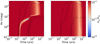 |
Fig. B.1 Spatio-temporal evolution of the sum of the abundances of the main C-bearing species (C+, C, CO, CH4, s-CO, and s-CH4) for model mHII:ini2 (left panel) and model mHHMC:ini2 (right panel). |
Furthermore, when we used the chemical network with 334 species, the sum of the main C-bearing species is 10−5 higher in abundance. In general, the abundance of the molecules at the frontier between the chemical regimes in model ini2 is lower with the larger network probably due to the presence of more complex species as well as the different initial abundances.
Appendix C Additional figures
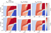 |
Fig. C.1 Spatio-temporal evolution of the abundances for HCN for models mHII:p2.5 (top panels) and mHII:p1 (bottom panels) with models r0.015 (left panels), models r0.05 (middle panels) and models r0.10 (right panels). Contours are plotted: solid line for the Td (30, 100 and 150 K) and dashed lines for G (10−1 and 103 Draine unit). |
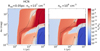 |
Fig. C.2 Spatio-temporal evolution of the abundances for HCN for the reference model mHII:n7 (left panel) and models n6 (right panel). Contours are plotted: solid line for the Td (30, 100 and 150 K) and dashed lines for G (10−1 and 103 Draine unit). |
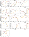 |
Fig. C.3 Change of the size of the ionized cavity r0.015, r0.05 and r0.10: Time evolution of the integrated intensities of the selected species listed in Table 5. Model mHII is represented with solid line and model mHHMC with dashedline. Model r0.015 is represented in brown, model r0.05 in black, and model r0.10 in yellow. |
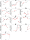 |
Fig. C.4 Change of density at the ionization front n7 and n6: Time evolution of the integrated intensities of the selected species listed in Table 5. Model mHII is represented with solid line and model mHHMC with dashed line. Model n7 is represented in black and model n6 in red. |
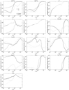 |
Fig. C.5 Change of the initial abundances ini1 and ini2: Time evolution of the integrated intensities of the selected species listed in Table 5. Model mHII is represented with solid line and model mHHMC with dashed line. Model ini1 is represented in black and model ini2 in gray. |
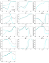 |
Fig. C.6 Change of the cut-off density of the modeling grid c1 and c6: Time evolution of the integrated intensities of the selected species listed in Table 5. Model mHII is represented with solid line and model mHHMC with dashed line. Model c1 is represented in black and model c6 in light blue. |
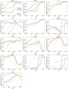 |
Fig. C.7 Change of the density profile p1: Time evolution of the integrated intensities of the selected species listed in Table 5. Model mHII:p1 is represented with solid line and model mHHMC:p1 with dashed line. Model r0.015 is represented in brown, model r0.05 in black, and model r0.10 in yellow. |
References
- Akimkin, V. V., Kirsanova, M. S., Pavlyuchenkov, Y. N., & Wiebe, D. S. 2015, MNRAS, 449, 440 [NASA ADS] [CrossRef] [Google Scholar]
- Beuther, H., Churchwell, E. B., McKee, C. F., & Tan, J. C. 2007, in Protostars and Planets V, eds. B. Reipurth, D. Jewitt, & K. Keil (Tucson: University of Arizona Press), 165 [Google Scholar]
- Bruderer, S., Benz, A. O., Bourke, T. L., & Doty, S. D. 2009a, A&A, 503, L13 [NASA ADS] [CrossRef] [EDP Sciences] [Google Scholar]
- Bruderer, S., Benz, A. O., Doty, S. D., van Dishoeck, E. F., & Bourke, T. L. 2009b, ApJ, 700, 872 [NASA ADS] [CrossRef] [Google Scholar]
- Cesaroni, R., Pestalozzi, M., Beltrán, M. T., et al. 2015, A&A, 579, A71 [NASA ADS] [CrossRef] [EDP Sciences] [Google Scholar]
- Choudhury, R., Schilke, P., Stéphan, G., et al. 2015, A&A, 575, A68 [NASA ADS] [CrossRef] [EDP Sciences] [Google Scholar]
- Churchwell, E. 2002, ARA&A, 40, 27 [Google Scholar]
- De Pree, C. G., Peters, T., Mac Low, M.-M., et al. 2014, ApJ, 781, L36 [NASA ADS] [CrossRef] [Google Scholar]
- Didelon, P., Motte, F., Tremblin, P., et al. 2015, A&A, 584, A4 [NASA ADS] [CrossRef] [EDP Sciences] [Google Scholar]
- Draine, B. T. 1978, ApJS, 36, 595 [NASA ADS] [CrossRef] [Google Scholar]
- Draine, B. T.,& Bertoldi, F. 1996, ApJ, 468, 269 [NASA ADS] [CrossRef] [EDP Sciences] [Google Scholar]
- Dullemond, C. P., Juhasz, A., Pohl, A., et al. 2012, Astrophysics Source code Library [record ascl:1202.015] [Google Scholar]
- Fuente, A., Martin-Pintado, J., Cernicharo, J., & Bachiller, R. 1993, A&A, 276, 473 [NASA ADS] [Google Scholar]
- Garrod, R. T. 2008, A&A, 491, 239 [NASA ADS] [CrossRef] [EDP Sciences] [Google Scholar]
- Garrod, R. T. 2013, ApJ, 765, 60 [Google Scholar]
- Garrod, R. T., & Herbst, E. 2006, A&A, 457, 927 [NASA ADS] [CrossRef] [EDP Sciences] [Google Scholar]
- Garrod, R. T., Wakelam, V., & Herbst, E. 2007, A&A, 467, 1103 [NASA ADS] [CrossRef] [EDP Sciences] [Google Scholar]
- Gaume, R. A., Goss, W. M., Dickel, H. R., Wilson, T. L., & Johnston, K. J. 1995, ApJ, 438, 776 [NASA ADS] [CrossRef] [Google Scholar]
- Goldsmith, P. F., Irvine, W. M., Hjalmarson, A., & Ellder, J. 1986, ApJ, 310, 383 [NASA ADS] [CrossRef] [PubMed] [Google Scholar]
- Graninger, D. M., Herbst, E., Öberg, K. I., & Vasyunin, A. I. 2014, ApJ, 787, 74 [NASA ADS] [CrossRef] [Google Scholar]
- Hasegawa, T. I., Herbst, E., & Leung, C. M. 1992, ApJS, 82, 167 [NASA ADS] [CrossRef] [Google Scholar]
- He, J., Shi, J., Hopkins, T., Vidali, G., & Kaufman, M. J. 2015, ApJ, 801, 120 [NASA ADS] [CrossRef] [Google Scholar]
- Herbst, E., & van Dishoeck E. F. 2009, ARA&A, 47, 427 [NASA ADS] [CrossRef] [Google Scholar]
- Herbst, W., & Racine, R. 1976, AJ, 81, 840 [NASA ADS] [CrossRef] [Google Scholar]
- Hoare, M. G., Kurtz, S. E., Lizano, S., Keto, E., & Hofner, P. 2007, in Protostars and Planets V, eds. B. Reipurth, D. Jewitt, & K. Keil (Tucson: University of Arizona Press), 181 [Google Scholar]
- Hosokawa, T., & Omukai, K. 2009, ApJ, 691, 823 [NASA ADS] [CrossRef] [Google Scholar]
- Jin, M., Lee, J.-E., & Kim, K.-T. 2015, ApJS, 219, 2 [NASA ADS] [CrossRef] [Google Scholar]
- Jing, D., He, J., Brucato, J. R., et al. 2012, ApJ, 756, 98 [NASA ADS] [CrossRef] [Google Scholar]
- Kurtz, S. 2005, in Massive Star Birth: A Crossroads of Astrophysics, eds. R. Cesaroni, M. Felli, E. Churchwell, & M. Walmsley, IAU Symp., 227, 111 [NASA ADS] [CrossRef] [Google Scholar]
- Kurtz, S., Cesaroni, R., Churchwell, E., Hofner, P., & Walmsley, C. M. 2000, Protostars and Planets IV, eds. V. Mannings, A. P. Boss, S. S. Russell (Tucson: University of Arizona Press), 299 [Google Scholar]
- Laor, A., & Draine, B. T. 1993, ApJ, 402, 441 [NASA ADS] [CrossRef] [Google Scholar]
- Le Bourlot, J., Le Petit, F., Pinto, C., Roueff, E., & Roy, F. 2012, A&A, 541, A76 [NASA ADS] [CrossRef] [EDP Sciences] [Google Scholar]
- Lee, H.-H., Herbst, E., Pineau des Forêts, G., Roueff, E., & Le Bourlot, J. 1996, A&A, 311, 690 [NASA ADS] [Google Scholar]
- Lee, S., Lee, J.-E., & Bergin, E. A. 2015, ApJS, 217, 30 [NASA ADS] [CrossRef] [Google Scholar]
- Le Petit, F., Nehmé, C., Le Bourlot, J., & Roueff, E. 2006, ApJS, 164, 506 [NASA ADS] [CrossRef] [EDP Sciences] [Google Scholar]
- Lesaffre, P., Belloche, A., Chièze, J.-P., & André, P. 2005, A&A, 443, 961 [NASA ADS] [CrossRef] [EDP Sciences] [Google Scholar]
- Loison, J.-C., Wakelam, V., & Hickson, K. M. 2014, MNRAS, 443, 398 [Google Scholar]
- Noble, J. A., Theule, P., Mispelaer, F., et al. 2012, A&A, 543, A5 [NASA ADS] [CrossRef] [EDP Sciences] [Google Scholar]
- Paglione, T. A. D., Tosaki, T., & Jackson, J. M. 1995, ApJ, 454, L117 [NASA ADS] [CrossRef] [Google Scholar]
- Paglione, T. A. D., Jackson, J. M., & Ishizuki, S. 1997, ApJ, 484, 656 [NASA ADS] [CrossRef] [Google Scholar]
- Panoglou, D., Cabrit, S., Pineau Des Forêts, G., et al. 2012, A&A, 538, A2 [NASA ADS] [CrossRef] [EDP Sciences] [Google Scholar]
- Peters, T., Banerjee, R., Klessen, R. S., et al. 2010a, ApJ, 711, 1017 [NASA ADS] [CrossRef] [Google Scholar]
- Peters, T., Mac Low, M.-M., Banerjee, R., Klessen, R. S., & Dullemond, C. P. 2010b, ApJ, 719, 831 [NASA ADS] [CrossRef] [Google Scholar]
- Qin, S.-L., Schilke, P., Rolffs, R., et al. 2011, A&A, 530, L9 [NASA ADS] [CrossRef] [EDP Sciences] [Google Scholar]
- Rolffs, R., Schilke, P., Comito, C., et al. 2010, A&A, 521, L46 [NASA ADS] [CrossRef] [EDP Sciences] [Google Scholar]
- Sakai, S., Motome, Y., & Imada, M. 2009, Phys. Rev. Lett., 102, 056404 [NASA ADS] [CrossRef] [Google Scholar]
- Sánchez-Monge, Á., Beltrán, M. T., Cesaroni, R., et al. 2013a, A&A, 550, A21 [NASA ADS] [CrossRef] [EDP Sciences] [Google Scholar]
- Sánchez-Monge, Á., Kurtz, S., Palau, A., et al. 2013b, ApJ, 766, 114 [NASA ADS] [CrossRef] [Google Scholar]
- Schilke, P., Walmsley, C. M., Pineau Des Forêts, G., et al. 1992, A&A, 256, 595 [NASA ADS] [Google Scholar]
- Schmiedeke, A., Schilke, P., Möller, T., et al. 2016, A&A, 588, A143 [NASA ADS] [CrossRef] [EDP Sciences] [Google Scholar]
- Semenov, D., Hersant, F., Wakelam, V., et al. 2010, A&A, 522, A42 [NASA ADS] [CrossRef] [EDP Sciences] [Google Scholar]
- Sternberg, A., Le Petit, F., Roueff, E., & Le Bourlot J. 2014, ApJ, 790, 10 [NASA ADS] [CrossRef] [MathSciNet] [Google Scholar]
- Treviño-Morales, S. P. 2015, PhD Thesis, Universidad de Granada, http://hdl.handle.net/10481/42409 [Google Scholar]
- Treviño-Morales, S. P., Pilleri, P., Fuente, A., et al. 2014, A&A, 569, A19 [NASA ADS] [CrossRef] [EDP Sciences] [Google Scholar]
- Treviño-Morales, S. P., Fuente, A., Sánchez-Monge, Á., et al. 2016, A&A, 593, L12 [NASA ADS] [CrossRef] [EDP Sciences] [Google Scholar]
- Vasyunin, A. I., & Herbst, E. 2013, ApJ, 762, 86 [NASA ADS] [CrossRef] [Google Scholar]
- Visser, R., Kristensen, L. E., Bruderer, S., et al. 2012, A&A, 537, A55 [NASA ADS] [CrossRef] [EDP Sciences] [Google Scholar]
- Wakelam, V., & Herbst, E. 2008, ApJ, 680, 371 [NASA ADS] [CrossRef] [Google Scholar]
- Wang, M., Chin, Y.-N., Henkel, C., Whiteoak, J. B., & Cunningham, M. 2009, ApJ, 690, 580 [NASA ADS] [CrossRef] [Google Scholar]
- Wilson, T. L.,& Rood, R. 1994, ARA&A, 32, 191 [NASA ADS] [CrossRef] [Google Scholar]
- Wood, D. O. S., & Churchwell, E. 1989, ApJS, 69, 831 [NASA ADS] [CrossRef] [Google Scholar]
- Ziurys, L. M., & Turner, B. E. 1986, ApJ, 300, L19 [NASA ADS] [CrossRef] [PubMed] [Google Scholar]
For consistency reasons we employ the same predecessor version of Pandora that Choudhury used in their benchmark study. A full integration into Pandora is currently underway.
The gas to dust mass ratio is assumed to be 100 in the models.
Hereafter we will use HII region model to refer to this model although the ionized gas is only used as a boundary condition.
Differential Variable-coefficient Ordinary Differential equation solver with the Preconditioned Krylov method GMRES for the solution of linear systems; http://www.netlib.org/ode.
The prefix s- indicates grain surface species, we will use this notation throughout the paper.
HC15N is optically thick from 104 to 3 × 10⁴ yr.
The free-free continuum was not included, which would result in the lines being seen in absorption in the HII region model.
We refer several times in this paper to observations with the IRAM 30 m telescope because of the spectral survey of the UCHII region Monoceros R2 made by Treviño-Morales et al. (2014, 2016) with this telescope. An outlook of this work will be to produce a model of Monoceros R2 and compare the results with the observations.
All Tables
Initial abundances of the principal species used in the models are shown in the second and third columns.
H2 dissociation front position from the ionization front at 105 yr for the different models.
List of selected species, one of their transition and the corresponding frequency in GHz.
Initial abundances of the principal species used in the models are shown in Col. 2 for a chemical network of 183 species and in Col. 3for 334 species.
All Figures
|
Fig. 1 Flowchart showing the setup of the variant of the modeling framework Pandora (Schmiedeke et al. 2016) employed here. |
| In the text | |
|
Fig. 2 Left: sketch of the real geometry of the HII region in the presence of accretion (based on models by Peters et al. 2010a,b). Right: our approximation by a spherical HII region filled with electrons and ions, but no dust. The PDR and the molecular gas surrounding the HII region are not represented in the sketches. Since the accretion disk does not cover a large fraction of the volume, and does not shield a large part of the spherical surface, we deem the approximation by a spherical region a reasonable approach, which greatly facilitates the calculation, without deviating too much from the real situation. While Peters et al. (2010a,b) show that the situation is dynamic and the shape varies on short timescales, following the true dynamics is beyond the current computational capabilities. We believe that, while the current static model is notstrictly correct, it still provides valuable insights into the process, even though it eventually will have to be superseded with a model incorporating the dynamics. |
| In the text | |
|
Fig. 3 Scheme of the HMC (left), HHMC (middle), and HII region (right) models. The spatio-temporal evolution of the radiation field is included in the computation of the relative abundances only for the HII region models. |
| In the text | |
|
Fig. 4 Time evolution of the parameters for an accreting massive proto-star with an accretion rate of 10−3 M⊙ s−1 (Hosokawa & Omukai 2009). The different panels show the mass of the star M* (top left), the star radius R* (top right), the total luminosity Ltot (bottom left) and the effective temperature Teff (bottom right). |
| In the text | |
|
Fig. 5 Left panel: density distributions as a function of radius for a Plummer function with exponent γ = 2.5 (black) and γ = 1 (red) for the three sizes of HII regions: 0.015 (solid), 0.05 (dashed), 0.10 pc (dash-dotted). Right panel: visual extinction as a function of radius. |
| In the text | |
|
Fig. 6 Spatio-temporal evolution of the dust temperature (left) and radiation field intensity (right) in the case of the reference model mHII:r0.05n7ini1c1p2.5s183. Contours are plotted: solid line for Td (30, 100 and 200 K) and dashed lines for G (10−1, 103 and 106 Draine unit). |
| In the text | |
|
Fig. 7 Spatio-temporal evolution of the abundance of HCN for the model mHHMC:r0.05n7ini1c1p2.5s183 (left panels) and the corresponding model mHMC (right). Contours are plotted in solid line for Td (30, 100 and 200 K). |
| In the text | |
|
Fig. 8 Spatio-temporal evolution of the abundance of HCN (top panels) and C+ (bottom) for the reference model mHII (left panels) and model mHHMC (right). Contours are plotted: solid line for Td (30, 100 and 200 K) and dashed lines for G (10−1 and 103 Draine unit). |
| In the text | |
|
Fig. 9 Schematics showing the different regions in the HII region models (left) and in the HMC/HHMC models (right). |
| In the text | |
|
Fig. 10 Spatio-temporal evolution of the abundance of C4H2 and NH3 for the reference model mHII:ini1 (left panel) and model mHII:ini2 (right panel). Contours are plotted: solid line for Td (20, 30, 100 and 150 K) and dashed lines for G (10−1 and 103 Draine unit). |
| In the text | |
|
Fig. 11 Time evolution of the HC15N (1–0) maps for the reference model mHII (top) and the associated model mHMC (bottom). The y-axis is the same as the x-axis. The bottom maps represent the same spectra convolved to the beam of the IRAM 30 m telescope. The convolved spectra have a weaker intensity. |
| In the text | |
|
Fig. 12 Example of the time evolution of CH3OH spectra around 337.6 GHz for the reference model mHII (black) and the associated model mHHMC (blue) and mHMC (green). Top: t = 1.5×10⁴ yr. Bottom: t = 7.46×10⁴ yr. |
| In the text | |
|
Fig. 13 Time evolution of the integrated intensities of all the species presented in Table 5. Model mHII is represented in black, model mHHMC in blue and model mHMC in green. The red dashed line represents the detectability threshold of 5 × 10⁻² K km s−1 obtained with an assumed rms noise of 3 mK. |
| In the text | |
|
Fig. 14 Schematic summarizing the results of the time evolution of the integrated intensities for the different models: size of the ionized cavity and density profile (top panel), density at the ionization front (second panel), initial abidances (third panel) and cut-off density (bottom panel). Lines with the integrated intensity Iint > 100 are represented in green, 10 < Iint < 100 in yellow, 1 < Iint < 10 in orange and Iint < 1 K km s−1 in red. Undetected lines, with integrated intensities lower than the detectability threshold of 5 × 10⁻² K km s−1, are represented in gray. |
| In the text | |
|
Fig. 15 Spatio-temporal evolution, focused between 100 and 105 yr, of the abundance ratio [HNC]/[HCN] for the reference model mHII (left) and the corresponding mHHMC model (right). Contours are plotted for Td (20, 30, 40, 50, 100 and 150 K). The bottom panels show the same results for [HN13 C]/[HC15N]. |
| In the text | |
|
Fig. 16 Time evolution for the reference model mHII (black), mHHMC (blue) and mHMC (green) of integrated intensity ratio (HN13C (1–0)/HC15N (1–0)) |
| In the text | |
|
Fig. 17 Time evolution of the integrated intensities of HC15N, C+, C and NH3 (see the corresponding transition in Table 5). The reference model mHII is represented in black, model mHHMC in blue and model mHMC in green and the new HII region model in red. The red dashed line represents the detectability threshold of 5×10⁻² K km s−1 obtained with an assumed rms noise of 3 mK. |
| In the text | |
|
Fig. B.1 Spatio-temporal evolution of the sum of the abundances of the main C-bearing species (C+, C, CO, CH4, s-CO, and s-CH4) for model mHII:ini2 (left panel) and model mHHMC:ini2 (right panel). |
| In the text | |
|
Fig. C.1 Spatio-temporal evolution of the abundances for HCN for models mHII:p2.5 (top panels) and mHII:p1 (bottom panels) with models r0.015 (left panels), models r0.05 (middle panels) and models r0.10 (right panels). Contours are plotted: solid line for the Td (30, 100 and 150 K) and dashed lines for G (10−1 and 103 Draine unit). |
| In the text | |
|
Fig. C.2 Spatio-temporal evolution of the abundances for HCN for the reference model mHII:n7 (left panel) and models n6 (right panel). Contours are plotted: solid line for the Td (30, 100 and 150 K) and dashed lines for G (10−1 and 103 Draine unit). |
| In the text | |
|
Fig. C.3 Change of the size of the ionized cavity r0.015, r0.05 and r0.10: Time evolution of the integrated intensities of the selected species listed in Table 5. Model mHII is represented with solid line and model mHHMC with dashedline. Model r0.015 is represented in brown, model r0.05 in black, and model r0.10 in yellow. |
| In the text | |
|
Fig. C.4 Change of density at the ionization front n7 and n6: Time evolution of the integrated intensities of the selected species listed in Table 5. Model mHII is represented with solid line and model mHHMC with dashed line. Model n7 is represented in black and model n6 in red. |
| In the text | |
|
Fig. C.5 Change of the initial abundances ini1 and ini2: Time evolution of the integrated intensities of the selected species listed in Table 5. Model mHII is represented with solid line and model mHHMC with dashed line. Model ini1 is represented in black and model ini2 in gray. |
| In the text | |
|
Fig. C.6 Change of the cut-off density of the modeling grid c1 and c6: Time evolution of the integrated intensities of the selected species listed in Table 5. Model mHII is represented with solid line and model mHHMC with dashed line. Model c1 is represented in black and model c6 in light blue. |
| In the text | |
|
Fig. C.7 Change of the density profile p1: Time evolution of the integrated intensities of the selected species listed in Table 5. Model mHII:p1 is represented with solid line and model mHHMC:p1 with dashed line. Model r0.015 is represented in brown, model r0.05 in black, and model r0.10 in yellow. |
| In the text | |
Current usage metrics show cumulative count of Article Views (full-text article views including HTML views, PDF and ePub downloads, according to the available data) and Abstracts Views on Vision4Press platform.
Data correspond to usage on the plateform after 2015. The current usage metrics is available 48-96 hours after online publication and is updated daily on week days.
Initial download of the metrics may take a while.