| Issue |
A&A
Volume 616, August 2018
|
|
|---|---|---|
| Article Number | A148 | |
| Number of page(s) | 19 | |
| Section | Stellar structure and evolution | |
| DOI | https://doi.org/10.1051/0004-6361/201832642 | |
| Published online | 05 September 2018 | |
Forward seismic modeling of the pulsating magnetic B-type star HD 43317
1
LESIA, Observatoire de Paris, PSL Research University, CNRS, Sorbonne Universités, UPMC Univ. Paris 06, Univ. Paris Diderot, Sorbonne Paris Cité, 5 Place Jules Janssen, 92195 Meudon, France
e-mail This email address is being protected from spambots. You need JavaScript enabled to view it.
2
Instituut voor Sterrenkunde, KU Leuven, Celestijnenlaan 200D, 3001 Leuven, Belgium
3
Department of Astrophysics, IMAPP, Radboud University Nijmegen, 6500 GL, Nijmegen, The Netherlands
4
Laboratoire AIM Paris-Saclay, CEA/DRF – CNRS – Université Paris Diderot, IRFU/DAp Centre de Saclay, 91191 Gif-sur-Yvette, France
Received:
15
January
2018
Accepted:
26
April
2018
Abstract
The large-scale magnetic fields detected at the surface of about 10% of hot stars extend into the stellar interior, where they may alter the structure. Deep inner regions of stars are only observable using asteroseismology. Here, we investigate the pulsating magnetic B3.5V star HD 43317, infer its interior properties and assess whether the dipolar magnetic field with a surface strength of Bp = 1312 ± 332 G causes different properties compared to those of non-magnetic stars. We analyze the latest version of the star’s 150 d CoRoT light curve and extract 35 significant frequencies, 28 of which are found to be independent and not related to the known surface rotation period of Prot = 0.897673 d. We perform forward seismic modeling based on non-magnetic, non-rotating 1D MESA models and the adiabatic module of the pulsation code GYRE, using a grid-based approach. Our aim was to estimate the stellar mass, age, and convective core overshooting. The GYRE calculations were done for uniform rotation with Prot. This modeling is able to explain 16 of the 28 frequencies as gravity modes belonging to retrograde modes with (ℓ, m) = (1, −1) and (2, −1) period spacing patterns and one distinct prograde (2, +2) mode. The modeling resulted in a stellar mass M⋆ = 5.8−0.2+0.1 M⊙, a central hydrogen mass fraction Xc = 0.54−0.02+0.01, and exponential convective core overshooting parameter fov = 0.004−0.002+0.014. The low value for fov is compatible with the suppression of near-core mixing due to a magnetic field but the uncertainties are too large to pinpoint such suppression as the sole physical interpretation. We assess the frequency shifts of pulsation modes caused by the Lorentz and the Coriolis forces and find magnetism to have a lower impact than rotation for this star. Including magnetism in future pulsation computations would be highly relevant to exploit current and future photometric time series spanning at least one year, such as those assembled by the Kepler space telescope and expected from the TESS (Continuous Viewing Zone) and PLATO space missions.
Key words: stars: magnetic field / stars: rotation / stars: oscillations / stars: early-type / stars: individual: HD 43317
© ESO 2018
1. Introduction
Large-scale magnetic fields are detected at the surface of about 10% of the observed early-type stars, that is, stars with spectral types O, B, or A (see e.g., Wolff 1968; Power 2007; Shultz et al. 2012, 2018; Wade et al. 2014; Grunhut & Neiner 2015). For the O, B, and A stars (which we refer to as hot stars), most magnetic detections are obtained by dedicated and systematic surveys using high-resolution spectropolarimetry (e.g., MiMeS, Wade et al. 2016). Magnetic candidates are discovered by indirect evidence of a large-scale magnetic field, such as rotational modulation caused by surface abundance inhomogeneities or magnetically confined matter in the circumstellar environment or by observed peculiar photospheric chemical abundances.
The majority of the detected large-scale magnetic fields have a simple geometry, often a magnetic dipole inclined to the rotation axis, with magnetic field strengths ranging from 100 G up to a few tens of kG. Because these large-scale magnetic fields are found to be stable over a time span of several decades, and because their properties do not scale with stellar parameters, they are thought to be created during the star formation process, that is, they have a fossil origin (e.g., Mestel 1999; Neiner et al. 2015). Results of both semi-analytical descriptions and numerical simulations have demonstrated that the magnetic field detected at the surface must extend deep within the radiative envelope of hot stars to ensure the stability of these magnetic fields (see e.g., Markey & Tayler 1973; Duez et al. 2010; Braithwaite 2004, 2006, 2007, 2008; Featherstone et al. 2009; Duez & Mathis 2010). These (large-scale) magnetic fields may influence the stellar structure due to the Lorentz force, in addition to the pressure force and gravity. Theoretical work suggests that the internal properties of a large-scale magnetic field would impose uniform rotation within the radiative layers (e.g., Ferraro 1937; Moss 1992; Spruit 1999; Mathis & Zahn 2005; Zahn 2011). As such, it is expected that matter loses its inertia quicker when overshooting the convective core boundary than in the absence of a magnetic field (e.g., Press 1981; Browning et al. 2004). Therefore, the presence of magnetic forces should result in a smaller convective core overshooting region.
Aside from isochrone fitting of binaries or clusters, asteroseismology is an excellent method to probe the internal stellar structure from the interpretation of detected stellar oscillations (Aerts et al. 2010). This is particularly true when estimating core overshooting from gravity (g) modes, as these are most sensitive to the deep stellar interior. About 15 magnetic pulsating stars with a spectral type earlier than B3 have been discovered so far (e.g., Buysschaert et al. 2017a). This is mainly due to the fact that only ~10% of hot stars are magnetic and that seismic data are available for only a few such stars. In addition, the presence of a very strong magnetic field may influence the driving and damping of pulsation modes and waves (e.g., Lecoanet et al. 2017). Of the hottest known magnetic pulsating stars, only β Cep (Shibahashi & Aerts 2000; Henrichs et al. 2013) and V2052 Oph (Neiner et al. 2012; Handler et al. 2012; Briquet et al. 2012) have been studied using combined asteroseismic and magnetometric analyses (i.e., magneto-asteroseismology). These two stars are both pressure-mode (p-mode) pulsators. The study of V2052 Oph demonstrated that this magnetic pulsating star has a smaller convective core overshooting layer compared to the similar yet non-magnetic pulsator θOph (Briquet et al. 2007), as expected from theoretical predictions.
In this paper, we selected the B3.5V star HD 43317 for detailed forward seismic modeling because it has a well characterized large-scale magnetic field (Briquet et al. 2013; Buysschaert et al. 2017b), and, most importantly, its CoRoT light curve (Convection Rotation and planetary Transits; Baglin et al. 2006) shows a rich frequency spectrum of many g-mode frequencies (Pápics et al. 2012). The spectroscopy of HD 43317 suggested it to be a single star and the spectroscopic analysis indicated a solar-like metallicity, an effective temperature Teff = 17 350 ± 750 K and a surface gravity log g = 4.0 ± 0.1 dex (Pápics et al. 2012). Furthermore, the measured rotation velocity is v sin i = 115 ± 9 km s−1 (Pápics et al. 2012) and the rotation period is Prot = 0.897673(4) d (Buysschaert et al. 2017b). From this work, it was also found that the dipolar magnetic field at the surface of HD 43317 has a strength of 1.0–1.5 kG, which should be strong enough to result in uniform rotation in the radiative layer according to theoretical criteria (Buysschaert et al. 2017b). We note that most studied B- and F-type g-mode pulsators with asteroseismic core-to-envelope rotation rates rotate almost uniformly. The studied sample with such measurements contains stars that rotate up to about half their critical rotation rate but magnetic measurements are not available for them (Aerts et al. 2017; Van Reeth et al. 2018).
In this paper, we assess the interior properties of HD 43317 from its g modes. Since the CoRoT data underwent a final end- of-life reduction to produce the version of the light curves in the public data archive, we performed a new frequency extraction in Sect. 2 to obtain a conservative list of candidate pulsation mode frequencies. Section 3 treats the detailed forward modeling of HD 43317 by coupling one-dimensional (1D) stellar structure models with pulsation computations, adopting various hypotheses as explained in the text. We discuss the results and implications of the forward modeling in Sect. 4, and summarize and draw conclusions in Sect. 5.
2. Frequency extraction
2.1. CoRoT light curve
CoRoT observed HD 43317 during campaign LRa03 from 30/09/2009 until 01/03/2010, producing high-cadence, high-precision space-based photometry (see Auvergne et al. 2009, for explicit details on the spacecraft and its performance). The total light curve spanned 150.49 d with a median observing cadence of 32 s and was retrieved from the CoRoT public archive1. An earlier version of the light curve was analyzed by Pápics et al. (2012) to study the photometric variability of HD 43317.
We re-processed the CoRoT light curve by removing obvious outliers indicated by a non-zero status flag. We also removed the so-called “in-pasted” observations added by the CoRoT data center to fill observing gaps. Further, we performed a correction for the (likely instrumental) long-term variability through application of a local linear regression filter, removing all signal with a frequency below 0.05 d−1. We ensured that the periodic variability detected in the data was well above this value and that the amplitudes of the frequencies were not significantly altered by the applied correction. Finally, we converted the flux to parts- per-million (ppm). This corrected light curve is shown in the top panel of Fig. 1. Its Rayleigh frequency resolution amounts to δfray = 1/150.49 = 0.00665 d−1.
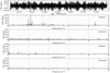 |
Fig. 1. CoRoT light curve (top) and the corresponding Lomb-Scargle periodograms (2nd and 4th row for increased visibility) of HD 43317. The 35 significant frequencies are indicated by the red tick marks in the upper parts of the periodogram panels. Corresponding periodograms of the residual light curve are given in panels on the 3rd and 5th row. |
2.2. Iterative prewhitening
We used the corrected CoRoT light curve to determine the frequencies and amplitudes of the periodic photometric variability by means of iterative prewhitening. This approach is appropriate for intermediate- and high-mass pulsators (e.g., Degroote et al. 2009). To deduce the significance of a frequency in the tentimes oversampled Lomb-Scargle periodogram (Lomb 1976; Scargle 1982), we relied on its signal-to-noise ratio (S/N) level. A frequency was accepted if it had a S/N ≥ 4 in amplitude (Breger et al. 1993), where the noise level was computed in a frequency window of 1 d−1 centered at the frequency peak after its corresponding variability was prewhitened. It has been demonstrated (see e.g., Degroote et al. 2009; Pápics et al. 2012; Degroote et al. 2012) that such a S/N criterion is more appropriate than the false alarm probability (i.e., p-criterion) due to the correlated nature and the noise properties of CoRoT data. The narrow frequency window of 1 d−1 was chosen over wider frequency windows to have a conservative frequency list for the subsequent modeling procedure.
We performed the iterative prewhitening in the frequency domain spanning from 0 to 10 d−1. No significant pulsation frequencies occurred at higher values, and aliasing structure due to the satellite-orbit frequency at fsat = 13.97 d−1 is not of interest for the interpretation of the modes. In total, we deduced 35 significant frequencies with values ranging from 0.2232 d−1 up to 6.3579 d−1. We provide the optimised frequency and amplitude values after non-linear least-squares fitting in the time domain in Table 1, as well as their corresponding S/N values. We also mark these frequencies in the periodogram of the CoRoT light curve, together with the periodogram of the residual light curve, in Fig. 1. The formal frequency and amplitude errors following the method of Montgomery (1999) were calculated, and these formal errors are also listed in Table 1. We recall that amplitudes were not used in the subsequent modeling. It is well known that such formal error estimates grossly underestimate the true errors, because of the simplistic assumption of uncorrelated data with white Gaussian noise. This underestimation is particularly prominent in the case of CoRoT data for g-mode pulsators, as these are highly correlated in nature and are subject to heteroscedastic errors (see Degroote et al. 2009). Correcting for these two properties is far from trivial but leads to an increase in frequency errors of at least one and possibly two orders of magnitude (Table 1).
2.3. Selecting the individual mode frequencies
Forward seismic modeling is commonly done by fitting the frequencies of independent pulsation modes. Therefore, the frequencies extracted from the CoRoT photometry of HD 43317 by the iterative prewhitening needed to be filtered for combination frequencies. For this reason, we limited the frequency list to values that could not be explained by frequency harmonics or low-order (2 or 3) linear combinations of the five highest amplitude frequency peaks (following the method of e.g., Kurtz et al. 2015; Bowman 2017). Low-order combination or harmonic frequencies typically have a smaller amplitude than the individual parent mode frequencies. Therefore, we identified a frequency as a combination frequency if it had a smaller amplitude than the parent frequencies. We also excluded frequencies that corresponded to the known rotation frequency of the star, frot = 1.113991(5) d−1 (Buysschaert et al. 2017b), and its harmonics.
By using these various criteria, we removed a total of 7 frequencies from the list (see Table 1) and identified the remaining 28 as candidate pulsation mode frequencies for the forward seismic modeling.
3. Forward seismic modeling
3.1. Setup
To determine the stellar structure of HD 43317, we computed a grid of non-rotating, non-magnetic 1D stellar structure and evolution models employing MESA (v8118, Paxton et al. 2011, 2013, 2015). For each MESA model in the grid, we computed linear adiabatic pulsation mode frequencies of dipole and quadrupole geometries using the pulsation code GYRE (v4.1, Townsend & Teitler 2013). These theoretical predictions for the pulsation mode frequencies were then quantitatively compared to the frequencies extracted from the CoRoT light curve to deduce the best fitting MESA models. Such a grid-based modeling approach has successfully been used to interpret the pulsation mode frequencies of g-mode pulsations in rotating stars based on Kepler space photometry (e.g., Van Reeth et al. 2016 for Dor pulsators and Moravveji et al. 2016 for SPB stars). A good grid setup requires appropriate evaluation of the effect of the choices for the input physics of stellar models on the predicted pulsation frequencies. For g modes in stars with a convective core, a global assessment for non-magnetic pulsators was recently offered by Aerts et al. (2018). These authors showed that typical uncertainties for the theoretical predictions of low-degree g-mode pulsation frequencies range from 0.001 to 0.01 d−1, depending on the specific aspect of the input physics that is being varied. The grid of MESA models in this paper was constructed accordingly.
Compared to the forward modeling of rotating g-mode pulsators based on Kepler space photometry, the case of HD 43317 is hampered by two major limitations: i) the ten times poorer frequency resolution of the data that led to fewer significant frequencies and prevented mode identification from period spacing patterns; and ii) the unknown effect of a magnetic field in the theoretical prediction of the pulsation frequencies. For this reason, the MESA grid was limited to the minimum number of free stellar parameters to be estimated for meaningful seismic modeling: the stellar mass M⋆, the central hydrogen mass fraction Xc (as a good proxy for the age), and the convective core overshooting. For the latter, we used an exponential overshooting description with parameter fov. Each of these three parameters were allowed to vary in a sensible range appropriate for B-type g-mode pulsators and using discrete steps. The stellar mass ranged from 4.0 M⊙ to 8.0 M⊙, with a step of 0.5 M⊙. For each of these masses, MESA models were evolved from the zero-age main-sequence (ZAMS), corresponding to Xc ~ 0.70, to the terminal-age main-sequence (TAMS), defined as Xc = 0.001; we saved the stellar structure models at discrete Xc steps of 0.01. The parameter for the exponential convective core overshooting, fov, is a dimensionless quantity expressed in units of the local pressure scale height; it was varied from 0.002 up to 0.040, with a step of 0.002. We refer to Freytag et al. (1996), Herwig (2000) and Pedersen et al. (2018) for explicit descriptions of this formulation of core overshooting. We followed the method of Pedersen et al. (2018) to set the exponential overshooting in MESA, where we employed a f0 = 0.005. All other aspects of the input physics were kept fixed according to the MESA inlist provided in Appendix A, following the guidelines in Aerts et al. (2018). In particular, a solar initial metallicity was adopted according to the spectroscopic results based on a NLTE abundance analysis by Pápics et al. (2012). The chemical mixture was taken to be the solar one from Asplund et al. (2009). We used the opacity tables from Moravveji (2016). Further, we relied on the Ledoux criterion to determine the convection boundaries and adopted the mixing length theory by Cox & Giuli (1968), with mixing length parameter αmlt = 2.0 based on the solar calibration by Christensen-Dalsgaard et al. (1996). We fixed the semi-convection parameter αsc = 0.01 and included additional constant diffusive mixing in the radiative region Dext = 10 cm2 s−1 following Moravveji et al. (2016). The MESA computations were started from pre-computed pre-main sequence models that come with the installation suite of the code.
For each of the MESA models in the grid, we computed the adiabatic pulsation frequencies for dipole (ℓ = 1) and quadrupole (ℓ = 2) g modes with GYRE, given that recent Kepler data of numerous rotating F- and B-type g-mode pulsators all revealed such low-degree modes (e.g., Van Reeth et al. 2016; Pápics et al. 2017; Saio et al. 2017). The effects of rotation on the pulsation mode frequencies were included in the GYRE calculations by enabling the traditional approximation (see e.g., Eckart 1960; Townsend 2003). While doing so, we assumed that the star is a rigid rotator with frot = 1.113991 d−1, as determined from the magnetometric analysis (at the stellar surface) by Buysschaert et al. (2017b) and following the findings by Aerts et al. (2017) and Van Reeth et al. (2018). We computed all dipole and quadrupole g modes with radial orders from ng = −1 to ng = −75. The settings for the GYRE computations are contained in Appendix B.
We adopted a quantitative frequency-matching approach and compared the GYRE pulsation mode frequencies with the observed CoRoT frequencies, as is common practice in forward seismic modeling. As such, we determined the closest model frequency to an observed frequency, and used these to compute the reduced χ2 value of the fit. While doing so, any predicted model frequency was allowed to match only one observed frequency. The reduced χ2 values were defined as: (1)
(1)
with N > 4 the total number of frequencies included in the fit, k = 3 the number of free parameters to estimate (i.e., the three input parameters of the MESA grid),  the considered detected frequency in the CoRoT data,
  the theoretically predicted GYRE pulsation mode frequency, and δf
ray the Rayleigh frequency resolution of the CoRoT light curve. The square of the latter was taken to be a good overall estimate of the variance that encapsulated the frequency resolution of the CoRoT data and the errors on the theoretical frequency predictions by GYRE, given that the formal errors in Table 1 were unrealistically small and the theoretical predictions were of similar order of magnitude to the Rayleigh limit for the data set of HD 43317. Moreover, due to lack of an a priori mode identification and evolutionary status of the star, it was seen as recommendable to give equal weight to each of the detected frequencies in the fitting procedure because the mode density varies considerably during the evolution along the main sequence. We discuss this issue further in the following sections.
the theoretically predicted GYRE pulsation mode frequency, and δf
ray the Rayleigh frequency resolution of the CoRoT light curve. The square of the latter was taken to be a good overall estimate of the variance that encapsulated the frequency resolution of the CoRoT data and the errors on the theoretical frequency predictions by GYRE, given that the formal errors in Table 1 were unrealistically small and the theoretical predictions were of similar order of magnitude to the Rayleigh limit for the data set of HD 43317. Moreover, due to lack of an a priori mode identification and evolutionary status of the star, it was seen as recommendable to give equal weight to each of the detected frequencies in the fitting procedure because the mode density varies considerably during the evolution along the main sequence. We discuss this issue further in the following sections.
During the forward modeling of HD 43317, the χ2 value of the fit to the GYRE frequencies of a given MESA model was not the only diagnostic. We also considered the location of the best MESA models (i.e., those with the lowest χ2 value) in the Kiel diagram to investigate how unique the best solution was. In case the parameters of the MESA models were well constrained by the fitting process, we anticipated the best models to lie within the same location in the Kiel diagram representing a unique χ2 valley in the 3D parameter space of the MESA grid, which then allowed us to create simplistic confidence intervals for the free parameters, as explained below. This method was a necessary complication compared to the modeling of Kepler stars because no obvious independent period spacing pattern spanning several consecutive radial orders could be identified for HD 43317. Therefore, the straightforward method for mode identification using the technique employed by Van Reeth et al. (2015, 2016) was not possible for our CoRoT target star.
3.2. Blind forward modeling
Although the CoRoT data were sufficient to detect g modes in B-type stars, the relatively large Rayleigh frequency resolution did not allow for unambiguous mode identification in the case of HD 43317 due to its fast rotation. This is different from the case of the CoRoT ultra-slow rotator HD 50230, whose g-mode periods constituted the first discovered period spacing pattern that led to mode identification for a main sequence star thanks to the absence of a slope in its pattern (Degroote et al. 2010). However, although not available for HD 43317, the ten-times-longer light curves observed by the Kepler mission for tens of g-mode pulsators meanwhile provided critical information on the types of modes expected in such rapidly rotating pulsators (e.g., Van Reeth et al. 2015; Pápics et al. 2017; Saio et al. 2017, for sample papers with B- and F-type stars). This led these authors to the conclusion that almost all detected g modes were dipole or quadrupole modes, irrespective of the rotation rate of the g-mode pulsator. We relied on this knowledge from Kepler to guide and perform our modeling of HD 43317.
Without a period spacing pattern to identify (some of) the 28 candidate pulsation mode frequencies, we first permitted the observed frequencies to match with any of the theoretical frequencies of the predicted dipole or quadrupole mode geometries for a given MESA model, without taking the constraints from spectroscopy into account. The locations of the 20 models with the lowest χ2 value resulting from such “blind” modeling in the Kiel diagram are shown in Fig. 2. These models corresponded to various stellar masses, spanning the entire MESA grid. Moreover, the lowest χ2 < 1 were reached for models with a low Xc value, corresponding to the lower log g values in the grid. This result is a common feature of such unconstrained forward modeling without any restriction on the identification of the modes or on the evolutionary stage. Indeed, the mode density in the frequency region of interest is much higher for models near the TAMS than for less evolved stages (see Fig. 3). Therefore, the χ2 values will always be artificially smaller for evolved models near the TAMS than for less-evolved models in absence of mode identification. Moreover, the majority of these best models relied on zonal mode frequencies, while many of these are unresolved in the CoRoT data (see Fig. 3).
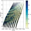 |
Fig. 2. Kiel diagram showing the results of blind forward modeling based on all 28 pulsation mode frequencies. The colour scale indicates the χ2 level and the black crosses represent the location of the 20 best fitting MESA models. The 1σ and 2σ confidence intervals for the derived spectroscopic parameters by Pápics et al. (2012) are shown by the black boxes. |
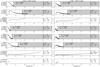 |
Fig. 3. Period spacing patterns, as computed by GYRE and accounting for rigid rotation at the rate of HD 43317, using the traditional approximation, for two demonstrative MESA models. Left: 6.5 M⊙ MESA model at the ZAMS; right: 4.0 M⊙ model close to the TAMS. Each row represents the theoretical period spacing pattern for a given mode geometry, with the range of radial orders as listed. Gray boxes correspond to regions where the frequency difference between theoretical frequencies of modes with consecutive radial order is smaller than the Rayleigh frequency resolution of the CoRoT data; these ranges cannot therefore be used. The corresponding pulsation period and radial order for the limiting theoretical mode to be used in the modeling for that given MESA model and mode geometry is listed in each upper left corner. |
This exercise illustrated that blind forward modeling without spectroscopic constraints is not a good strategy in the absence of mode identification. Indeed, the spectroscopic parameters of these best models did not agree with the observationally derived 2σ confidence intervals by Pápics et al. (2012), that is, Teff = 17 350 ± 1500 K and log g = 4.0 ± 0.25 dex. Therefore, a dedicated strategy for the forward seismic modeling of HD 43317 was required.
3.3. Conditional forward modeling
We adopted various hypotheses in the best model selection for the estimation of the three stellar parameters (M⋆, Xc, fov). The first hypothesis was that any selected MESA model should comply with the spectroscopic properties of the star. Therefore, we made sure that the effective temperature, Teff, and the surface gravity, log g, were consistent with those derived from high-precision spectroscopy. As such, we excluded any MESA models that did not agree with the 2σ confidence intervals of the combined spectroscopic analysis done by Pápics et al. (2012). This assumption resulted in the exclusion of MESA models near the TAMS, leaving only models with comparable mode density.
The next assumption was that any appropriate MESA model should be able to explain several of the highest-amplitude frequencies as pulsation mode frequencies. Indeed, it did not make sense to accept models that explained low-amplitude modes while they did not lead to a good description of the dominant modes. We (arbitrarily) placed the cut-off limit at an amplitude of 500 ppm, thus requiring that f9, f11, f13, and f31 were matched. Using spectroscopic mode identification techniques, Pápics et al. (2012) identified f31 to be a prograde (ℓ, m) = (2, +2) mode2. We therefore fixed the mode identification of this particular frequency during the modeling process. The other three dominant modes in the CoRoT photometry were not detected in the spectroscopy. This is not surprising given that photometric and spectroscopic diagnostics are differently affected by mode geometries (see Chapter 6 in Aerts et al. 2010) and that we have no information on the intrinsic amplitudes of excited modes. Therefore, we were not able to use the identification of f31 to place constraints on the degree of the other highest-amplitude modes. However, given the dominance of a sectoral mode in the spectroscopy, we excluded a pole-on view of the star, because it would correspond to an angle of complete cancellation for such a mode (at i = 0°; see e.g., Aerts et al. 2010). As such, Pápics et al. (2012) constrained the inclination angle to be iϵ [20°, 50°].
We considered different hypotheses on the identification of the modes, as described in the following sections. These hypotheses followed from comparison of the theoretical period spacing patterns with those from the detected frequencies (comparing Table 1 to Fig. 3). For most of the m > 0 modes, the frequency difference between modes of consecutive radial order was smaller or comparable to the Rayleigh limit of the CoRoT data. The same is true for most zonal modes, especially for the (ℓ, m) = (2, 0) modes. As such, creating a period spacing pattern spanning consecutive radial orders for such modes from the observed frequencies was not meaningful with the frequency resolution of the CoRoT data. Therefore, we assumed that the observed frequencies were m = −1 modes, unless explicit evidence was available (e.g., for f31 from spectroscopy). This was a valid assumption considering the results of Kepler for g-mode pulsators (Van Reeth et al. 2016) and the measured rotation rate of HD 43317. We then included additional observed frequencies under the made hypotheses.
With this piece-wise conditional modeling, we intended to constrain both the parameters of HD 43317 and the mode geometry of the detected frequencies. The theoretical period spacing patterns of the best models at any given step denoted which observed frequency could be additionally included in the frequency matching. Detected frequencies were considered for inclusion if they were sufficiently close to a theoretical frequency predicted by the best models. Ideally, this modeling scheme should lead to a well clustered group of MESA models in the Kiel diagram for a large number of the 28 detected frequencies, leading to an estimate on their mode geometry. To ensure robustness and reproducibility of a hypothesis during the forward seismic modeling, we defined the following criteria for any good solution:
-
At least five detected frequencies must be accounted for in the use of Eq. (1).
-
The location of the 20 best MESA models in the Kiel diagram must remain consistent with the 2σ spectroscopic error box.
3.4. Dipole retrograde mode hypothesis
As a first hypothesis, we considered the case that the three dominant pulsation mode frequencies, f9, f11, and f13, corresponded to dipole retrograde modes. Dipole modes were by far the most frequently detected ones in space photometry of g-mode pulsators (e.g., Pápics et al. 2014; Moravveji et al. 2016; Van Reeth et al. 2016). At the measured v sin i and frot of HD 43317, most of the detected g-mode frequencies in pulsators with Kepler photometry would belong to a series of (1, −1) modes (Van Reeth et al. 2016). As such, it was reasonable to assume that f9, f11, f13 were (1, −1) modes.
Using these three frequencies and f31 constrained by spectroscopy, the forward modeling led to models with a mass ranging from 5.0 M⊙ to 6.5 M⊙. A comparison of the observed frequencies with the model frequencies suggested that f11 was likely not a (1, −1) mode. We therefore dropped the requirement on this frequency and repeated the forward modeling with only f9 and f13 as (ℓ, m) = (1, −1) modes and f31 as a (2, +2) mode. This returned two families of solutions in the Kiel diagram, namely a group with M⋆ = 5.0 M⊙ and Xc ≈ 0.50, and a stripe of models with a mass of 5.5 M⊙, while Xc decreases from 0.63 to 0.52 and fov from 0.038 to 0.022. All these models resulted in similar theoretical (1, −1) frequencies and identified f29 as having this mode geometry as well. We therefore included this observed frequency in the hypothesis and repeated the forward modeling.
The modeling converged to only one family of solutions in the Kiel diagram that corresponded with M⋆ = 5.5 M⊙, Xc = 0.53−0.58 and fov ranging from 0.016 to 0.022. These models indicated that the observed frequencies f3, f4, f5, f6, f16 and f20 should be part of the (1, −1) period spacing pattern. We included only f4, because it was the closest match and repeated the modeling with the updated hypothesis.
We recovered the same set of 20 best MESA models with f4 included in the hypothesis and noted that five additional observed frequencies agreed with the theoretical predictions. Therefore, we satisfied our defined criteria. The conclusion of the modeling with this hypothesis is represented in Fig. 4. The top panel shows the Kiel diagram with the location of the 20 best MESA models, as well as the χ2 values of the fitting process to the theoretical GYRE frequencies. The model period spacing patterns of the 20 best fitted models (and the corresponding observed frequencies in the assumption) are given in the bottom panels of Fig. 4.
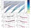 |
Fig. 4. Summary plot for the results of the forward modeling of HD 43317 based on the dipole mode hypothesis (see text). Top: Kiel diagram showing the location of the MESA models whose GYRE frequencies come closest to the detected frequencies. The color scale represents the χ2 value (see Eq. (1)), the open symbols indicate MESA models outside the spectroscopic limits of the star deduced by Pápics et al. (2012, with the 1σ and 2σ limits indicated by the black boxes) and the black crosses represent the location of the 20 best fitting MESA models. Bottom panels: period spacing patterns of the 20 best fitting MESA models for various mode geometries (black lines and squares). Those of the best description are shown in red. The observed pulsation mode periods used in the χ2 are indicated by the vertical gray lines, while the vertical blue regions indicate the observed period range taking into account the Rayleigh limit of the data. Only (1, −1) modes (i.e., f4, f9, f13, and f29, as well as the f31 as a (2, +2) mode) were relied upon to achieve the frequency matching. |
3.5. Increasing the mass resolution of the MESA grid
To investigate the robustness of our obtained solution shown in Fig. 4, we created a new grid of MESA models that had a finer mass resolution. This new grid had the same settings for the micro- and macro-physics as before, but the stellar masses ranged from 5.0 M⊙ up to 6.0 M⊙ with a step size of 0.1 M⊙. We repeated the frequency matching of the five observed frequencies to the GYRE frequencies of the finer grid of models and summarized the result in Fig. 5. The 20 best MESA models corresponded to slightly different values for the stellar mass and exponential overshooting factor. These values were unavailable in the coarser grid.
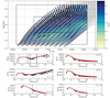 |
Fig. 5. Summary plot for the overall forward modeling of HD 43317 using the dipole mode hypothesis on the refined grid of MESA models. The same color scheme as in Fig. 4 is used. |
The theoretical frequencies for the already identified (1, −1) modes of the now 20 best models did not alter appreciably compared to those of the solution in the coarse grid, nor did the radial orders change. We included additional identifications as dipole modes, namely f5, f6, f8, f16, f20 and f32. The result of the modeling with these ten (1, −1) modes and one (2, +2) mode is illustrated in Fig. 6.
 |
Fig. 6. Summary plot for the overall forward modeling of HD 43317 using the extended dipole mode hypothesis on the refined grid of MESA models. The same color scheme as in Fig. 4 is used. |
We noted that the location of the 20 best MESA models now moved to slightly lower Xc values when using this more extended frequency list. However, the confidence intervals of these solutions for the different hypotheses still overlapped at a 2σ level, that is, the location of the best solutions did not move outside the range of their variance. Here, the α% confidence interval is defined by the upper limit on the χ2 value as (2)
(2)
where  is the χ2 value for the best fit and
  the tabulated value for an α% inclusion of the cumulative distribution function of a χ2 distribution with k = 3 degrees of freedom.
A local minimum in the χ2 landscape occurred for models with a stellar mass of 5.3 M⊙ and Xc ≈ 0.40 (i.e., Teff = 16 000 K and log g = 4.0 dex), but their χ2 values were larger than the upper limit of the 2σ confidence interval of the best solutions in the minimum dictated by the spectroscopic limits. This family of second-best models was only compatible at a 3σ level (see Fig. 8).
3.6. Adding modes with other mode geometry
At this stage, the theoretical frequencies of the best MESA models were able to explain 11 of the 28 observed frequencies of HD 43317. We studied whether yet unexplained detected frequencies could be associated to pulsation mode frequencies with a different geometry than (1, −1) modes. The frequency density argument made in Sect. 3.2 and indicated in Fig. 3 showed that it was impossible to resolve zonal and most m > 0 modes with the frequency resolution of the CoRoT data set. Therefore, we investigated whether theoretically predicted (ℓ, m) = (2, −1) modes could explain the additional detected frequencies. Such modes have an angle of least cancellation at 45° (Aerts et al. 2010). This was close to the updated value for the inclination angle i = 37 ± 3° derived in Sect. 4.1, validating this assumption. We identified five matches between theoretically predicted (2, −1) mode frequencies and the so far unused frequencies of HD 43317, namely f7, f11, f14, f15 and f21. These were subsequently included in the hypothesis and the modeling was repeated.
The result of this final modeling under the hypothesis that only (1, −1), (2, −1) and (2, +2) modes were observed in the CoRoT photometry of HD 43317 is summarized in Fig. 7. The location of the 20 best fitted MESA models did not change by including the five additional (2, −1) mode frequencies. The three estimated physical parameters, as well as some other output variables, are listed in Table 2 and the χ2 distributions for these parameters are shown in Fig. 8. Table 3 compares the observed frequencies with those predicted by GYRE based on the MESA model with the lowest χ2. This model has parameters M⋆ = 5.8 M⊙, Xc = 0.54, and fov = 0.004.
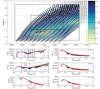 |
Fig. 7. Summary plot for the overall forward modeling of HD 43317 using the combined dipole mode hypothesis on the refined grid of MESA models. The same color scheme as in Fig. 4 is used. |
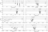 |
Fig. 8. Distribution of the χ2 values, computed during the forward seismic modeling of HD 43317 based on 16 of the 28 observed frequencies, using the refined grid of MESA models. The χ2 values for the 2σ and 3σ confidence intervals are indicated by the dotted and dashed black lines, respectively. The best 20 models are indicated by the black crosses. We refer to Table 2 for the description of the physical quantities. |
4. Discussion
4.1. Seismic estimation of the stellar parameters
Instead of using the discrete step size of the grid as the confidence intervals for M⋆, Xc, and fov as deduced from the forward modeling, we used the properties of the χ2 statistics. We computed the upper limit on the χ2 value for a 2σ confidence interval (i.e., 95.4% confidence interval) using Eq. (2). We included 16 frequencies in our final fitting process, resulting in 12 degrees of freedom, which led to  . This corresponds to the χ2 value of the best 19 MESA models (as shown in Fig. 8), supporting the visual inspection of the best models during the procedure. The corresponding confidence intervals on the parameters were
  , and
, and  . The skewed confidence intervals for M⋆ and fov resulted from a strong correlation between these parameters, as demonstrated in Fig. 9. We note that our grid of MESA models was limited from fov = 0.002 to 0.040, and therefore we could not exclude that fov had an even lower value than 0.002, in particular fov = 0.0. The MESA models within this χ2 valley had comparable values for the asymptotic period spacing pattern (see Table 2) defined as:
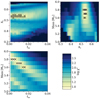 |
Fig. 9. Color maps indicating the pairwise (marginalized) correlation between the parameters in the (fine) grid of MESA models. Top left: correlation between Xc and fov after marginalizing over M⋆. Top right: correlation between M⋆ and Xc after marginalizing over fov. Bottom left: correlation between M⋆ and fov after marginalizing over Xc, indicating the strong correlation caused by models with the ΔΠ same value. The same color scale was used for all panels. The 20 best MESA models are indicated by the black crosses. |
 (3)
(3)
where N is the Brunt-Väisälä frequency, the integral is over the g-mode cavity, and ΔΠ is given in seconds (omitting the factor 2π in the definition). Comparable  values were caused by a similar value for the integral, following from the relation between the overall stellar mass and the mass inside the core and convective core overshooting region. We were unable to lift the degeneracy caused by this correlation without many more observed and well defined pulsation modes that had a different probing power in the near-core region. Additional observed trapped modes would be particularly helpful to achieve this, as they are most sensitive to the near-core layers. Such modes manifest themselves as regions of local minima in the period spacing patterns as observed with the Kepler satellite for numerous g-mode pulsators, but Kepler data have a ten-times-better frequency resolution than our CoRoT data.
Pápics et al. (2012) used the few dominant modes to estimate ΔΠ, without modeling the individual frequencies and while ignoring the rotation of the star. It turned out that we obtained a value about twice as high, pointing out the difficulty of deducing an appropriate ΔΠ value without good knowledge of the rotation frequency of the star. We emphasize that the high-precision frot value of HD 43317 determined from the magnetic modeling by Buysschaert et al. (2017b) was an essential ingredient for the successful seismic modeling of the star as presented here.
To investigate the pairwise correlation between the parameters of the grid of MESA models, we employed the marginalization technique to reduce the dimensionality of the χ2 landscape. This technique took the minimum χ2 value of the fit along the third axis of the grid, providing easily interpretable correlation maps (given in Fig. 9). These correlation maps indicated that the central hydrogen fraction, Xc, was well constrained, but these maps also illustrated the tight correlation between M⋆ and fov. These correlation maps also illustrated the existence of the (non-significant) secondary solution of MESA models, which was already apparent from the χ2 landscape in the Kiel diagram (see Fig. 7) and from the χ2 distribution of several parameters in Fig. 8. The bottom-left panel of Fig. 8 demonstrates that these models had a comparable value for ΔΠ to the global solution, thus explaining the reason why this secondary solution was (partly) retrieved.
The correlation between fov and M⋆ and the limited frequency resolution of the CoRoT data led to a relatively large confidence interval on the derived fov for HD 43317. The low value of the best model agreed well with the predictions from theory and simulations for hot stars hosting a detectable largescale magnetic field and with the only other observational result (i.e., V2052 Oph, Briquet et al. 2012). The 2σ confidence interval on fov was also compatible with the seismic estimate of this parameter for the non-magnetic B-type star KIC 10526294 (Moravveji et al. 2015, see their Fig. B.1). However, KIC 10526294 is a slow rotator with a rotation period of about 190 d, while HD 43317 is a rapid rotator. The result for fov from the seismic modeling of the B-type star KIC 7760680 (Moravveji et al. 2016, their Fig. 6) with Prot = 2.08 ± 0.04 d differs more than 2σ from the fov-value for HD 43317. Therefore, the forward seismic modeling of HD 43317 is compatible with the suppression of near-core mixing due to a large-scale magnetic field, but we could not exclude that other physical processes are involved in the limited overshooting, such as the nearcore rotation.
By construction of the best models, the seismic estimates for Teff and log g agreed well with the spectroscopic values by Pápics et al. (2012). The age estimate for the best model (28.4 Myr, see Table 2) is compatible with a literature value obtained from isochrone fitting to the spectroscopic parameters (i.e., 26 ± 6 Myr; Tetzlaff et al. 2011). Both results rely on stellar models that were computed with independent codes.
Further, we redetermined the inclination angle i using the radius of the best fitted MESA model (i.e., R = 3.39 R⊙), the value for v sin i = 115 ± 9 km s−1 (Pápics et al. 2012), and the rotation period Prot = 0.897673(4) d (Buysschaert et al. 2017b). This resulted in an inclination angle i = 37 ± 3°, where the largest uncertainty came from the estimate of v sin i. This a posteriori refinement of the inclination angle is compatible with the mode visibility of the dipole and quadrupole mode interpretation. With this inclination angle, we derived an updated value for the obliquity angle β = 81 ± 6°, employing the measurements for their longitudinal magnetic field of Buysschaert et al. (2017b) for the LSD profiles with their complete line mask. Using these angles, the longitudinal magnetic field measurements of Buysschaert et al. (2017b), the equation for the dipolar magnetic field strength of Schwarzschild (1950) and a linear limb-darking coefficient of u = 0.3 (appropriate for a B3.5V star, see e.g., Claret 2000), we deduced that the dipolar magnetic field of HD 43317 had a strength Bdip = 1312 ± 332 G. These values were all consistent with the ranges obtained by Buysschaert et al. (2017b), which were based on the range of acceptable inclination angles from Pápics et al. (2012).
4.2. Dependencies on the mode identification assumptions
During the forward seismic modeling, we were explicit on the assumptions about the mode geometry, and at which stage a given observed frequency entered the modeling scheme. Several of these frequencies did not have a unique mode identification (even for the best fitted MESA model). As an example, we discuss f15, which we assumed to be a (ℓ, m) = (2, −1) mode. However, the zonal mode frequency fng,ℓ,0 of f6 also matched closely with f15. Such a degeneracy occurred for several cases, but never in a systematic way. Moreover, these degeneracies did not significantly alter the confidence intervals of the parameters based on the selected MESA models as their corresponding GYRE frequencies were a good match with the observations. We considered it more sensible to use interrupted series of (1, −1) and (2, −1) modes (together with one (2, +2) mode confirmed by spectroscopy) during the forward seismic modeling of HD 43317 than to inject zonal modes that did not belong to any series in radial order or rotationally split multiplets. Finally, we emphasize that the assumption of the initial four (1, −1) modes with the spectroscopic identification of f31 and the enforced 2σ spectroscopic box sufficiently constrained the possible MESA models for HD 43317, while still complying with forward modeling results of Kepler B-type g-mode pulsators.
4.3. Assessment of the theoretical pulsation mode frequencies
In our computations of the mode frequencies, we made two important assumptions. The first one was uniform rotation, as the GYRE computations used the traditional approximation under this assumption. Following the results in Aerts et al. (2017) and in Van Reeth et al. (2018) for tens of g-mode pulsators, this was a valid assumption. Furthermore, uniform rotation in the radiative layer was theoretically predicted for stars with a stable largescale magnetic field (e.g., Ferraro 1937; Moss 1992; Spruit 1999; Mathis & Zahn 2005; Zahn 2011).
The second assumption was that we ignored the effect of the magnetic field on the g-mode frequencies because we did not have observational information on the interior properties of the large-scale magnetic field. Below we attempted to assess the consequences of these assumptions after we obtained a good model representing the stellar structure of the pulsating magnetic star HD 43317.
4.3.1. Frequency shifts of zonal modes due to the Coriolis force
For HD 43317, the independent measurement of the rotation frequency (at the stellar surface) was a necessary pre-requisite to be able to perform seismic modeling. Indeed, the well-known estimation procedure for frot from the period spacing patterns of g modes applied to Kepler data, as in Moravveji et al. (2016), Van Reeth et al. (2016) or Ouazzani et al. (2017), was not possible for our CoRoT target. Prior knowledge of the rotation frequency allowed us to apply the traditional approximation for rotation, which ignores the latitudinal component of the rotation vector. This approximation is appropriate for g modes in B- and F-type stars thanks to their large horizontal displacements, as long as they do not rotate too close to their critical rotation velocity (Ouazzani et al. 2017). However, forward modeling of such pulsators was so far also still done without taking into account the Coriolis force for slow rotators (cf., Moravveji et al. 2015; Schmid & Aerts 2016).
Here, we wish to compare the effects of ignoring the Coriolis and Lorentz forces for the resulting theoretical predictions of the g-mode frequencies, taking the case of HD 43317 as the only concrete example of a magnetic g-mode pulsator so far. Such comparison is most easily done for zonal modes (i.e., m = 0) of stellar models, as these are not subject to transformation effects between the co-rotating and inertial reference frames.
Unlike a first-order perturbative approach for the effects of the Coriolis force (e.g., Ledoux 1951), the traditional approximation results in frequency shifts for zonal pulsation modes. We computed the frequency differences for the zonal mode frequencies fng,ℓ,0 of the identified modes in the best MESA model with M⋆ = 5.8 M⊙, Xc = 0.54, and fov = 0.004, when ignoring or taking into account the Coriolis force. The results are listed in Table 3. As expected, the frequency shift due to the Coriolis force is large for the rotation rate of HD 43317. It increases with increasing radial order ng and with mode degree ℓ. For the pulsation modes with the highest ng values, the frequency-shifted value easily exceeded 25% of the non-rotating value fng,ℓ,0, clearly illustrating the need to account for the stellar rotation during the forward seismic modeling.
4.3.2. Frequency shifts of zonal modes due to the Lorentz force
To compute the shift in the pulsation mode frequency caused by an internal magnetic field, we followed the perturbative approach of Hasan et al. (2005), since it was one of the few available formalisms applicable to g modes. It assumes that the internal magnetic field corresponds to a poloidal axisymmetric field. While this is a limitation, there is currently no better prescription to apply.
Theoretical studies and numerical simulations showed that any extension of a large-scale magnetic field measured at the stellar surface towards the stellar interior needs to have both a toroidal and poloidal component of about equal strength to be stable over long time scales (e.g., Tayler 1980; Braithwaite 2006; Duez & Mathis 2010; Duez et al. 2010). However, Hasan et al. (2005) argued that the toroidal component of the internal magnetic field would lead to a lower frequency shift for high-radial order g modes than the poloidal component. Therefore, we adopted their formulation here. The resulting frequency shift can be expressed as (4)
(4)
where (5)
(5)
is the Alfvén frequency for an internal magnetic field with strength B0. This expression led to the magnetic splitting coefficient Sc, given as (6)
(6)
where ρc is the central mass density, R⋆ is the stellar radius, ω is the cyclic frequency (in rad s−1) corresponding to the angular pulsation mode frequency fng,ℓ,m and the Ledoux coefficients Cℓ,m have been introduced (see Ledoux & Simon 1957 and Eqs. (8) and (9) of Hasan et al. 2005). They describe the horizontal overlap between the g-mode displacement, assumed to be predominantly horizontal, with the dipolar magnetic field. Finally, I is defined as (7)
(7)
with x = r/R⋆ the radial coordinate, ξh(x) the horizontal displacement for the pulsation mode with frequency fng,ℓ,m, ρ(x) the internal density profile, and b(x) the profile of the magnetic field as a function of the radial coordinate. We followed the definition of Hasan et al. (2005) and assumed b(x) = (x/xc)−3, with xc the radial coordinate of the outer edge of the convective core. For our best model of HD 43317 (M⋆ = 5.8 M⊙, Xc = 0.54, and fov = 0.004), the MESA model delivered xc = 0.168.
We estimated the strength of the frozen-in large-scale magnetic field of HD 43317 at xc following the results provided by the simulations of Braithwaite (2008, we refer the reader to his Fig. 8). Depending on the age of the star, the internal magnetic field was 26.6 to 50.1 times as strong as at the stellar surface. Using our new estimate of the strength of the dipolar magnetic field at the surface of HD 43317, Bdip = 1312 ± 332 G, we obtained a near-core magnetic field strength in the range B0 = 26.1−82.4 kG. We computed the frequency shift using Eq. (4) for these two limiting values of B0, the model frequencies fng,ℓ,0 of the non-rotating case (see Table 3) and the difference in Ledoux constant ΔCℓ,m values to account for the mode geometry (similarly to Hasan et al. 2005). The values for the obtained frequency shifts due to the Lorentz force are given in Table 3 and are compared with the differences between the observed and the 20 best sets of model frequencies in Fig. 10.
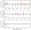 |
Fig. 10. Difference in frequency between the observed pulsation mode frequencies and the GYRE frequencies of the 20 best MESA models, ordered according to the mode geometry. The red squares indicate the difference between the observations and the best model description. The red vertical error bars indicate the frequency shift caused by an internal poloidal magnetic field of 82.4 kG and the red horizontal error bars represent the Rayleigh frequency resolution of the CoRoT light curve; both were often similar to the symbol size, while the magnetic frequency shift for the highest period dipole modes was larger than the indicated panel (see also Table 3). The black dashed and dotted lines show the Rayleigh frequency resolution and 3δfray, respectively. |
As expected from Eq. (4), we found that the frequency shifts depended on the strength of B0. Moreover, they increased with increasing radial order, since ω decreased and I increased. We found that the frequency shift was largest for the observed (1, −1) modes, since the difference in the Ledoux constants ΔCℓ,m were largest for such modes. All these results were compatible with those of Hasan et al. (2005).
The upper limit on the frequency shift due to the Lorentz force was almost always an order of magnitude smaller than that caused by the Coriolis force. Therefore, correctly accounting for the (uniform) rotation rate remained not only necessary, but was also more important during the forward modeling than accounting for a possible internal magnetic field that resulted from extrapolation of the surface field strength when dealing with field amplitudes such as the one measured for HD 43317. This can also be further understood when revisiting Eq. (4). First, the ratio of the Alfvén frequency and the pulsation mode frequencies were always very small (typically of the order of 10−9) permitting us to adopt a perturbative treatment of the effect of the Lorentz force on the pulsation modes. Most of the observed modes during the modeling were sub-inertial gravito-inertial modes (i.e., f < 2 frot). Therefore, they would be confined to an equatorial belt and thus propagate above a critical colatitude θc = arccos( f /(2 frot)) (see e.g., Townsend 2003). In the formalism by Hasan et al. (2005), the non-rotating approximation was assumed and modes were therefore expanded as spherical harmonics corresponding to modes propagating in the whole sphere. In this framework, the coefficient Cl,m evaluated the horizontal overlap of the oscillation mode with the magnetic field with positive integrals (we refer the reader to Eq. (7) in Hasan et al. 2005). As such, the determined frequency shifts due to the magnetic field should be larger in the case of the non-rotating approximation compared to equatorially trapped sub-inertial gravitoinertial modes. The modification of the radial term from the non-rotating case to the case of a sub-inertial case is more difficult to infer. However, if ωA ≪ 2Ω, it would not change the fact that the perturbative approach for the Lorentz force can be used.
In the case of super-inertial gravito-inertial modes (i.e., f > 2 frot), the situation would be much simpler since waves propagate in the whole sphere as in the non-rotating case and the eigenmodes would be less modified by the Coriolis acceleration (e.g., Lee & Saio 1997). Therefore, the evaluation of the frequency shift provided by Hasan et al. (2005) using the non-rotating assumption could be considered as a first reasonable step to evaluate the frequency shift induced by the Lorentz force. The next step would be to generalize their work using the traditional approximation to take into account the effect of the Coriolis acceleration on the oscillation modes, in particular in the sub-inertial regime. This would require a dedicated theoretical study and is far beyond the scope of the current paper.
We concluded, as an a posteriori check, that the working principle of our seismic modeling was acceptable for this star. Only for the higher-order dipole modes did the upper limit of the magnetic frequency shift become comparable with the frequency shift caused by the Coriolis force. Yet, only a few such pulsation mode frequencies were identified for HD 43317. In this case, a non-perturbative approach, as the one derived in Mathis & de Brye (2011), should be adopted.
Comparing the magnetic frequency shift with the differences between the observed and model frequencies (see Fig. 10) led to the conclusion that the current description of the frequency shifts due to the Lorentz force failed to improve the differences. This was not surprising given the simplification of the perturbative approach by Hasan et al. (2005), its assumptions on the geometry of the large-scale magnetic field, and because it neglects the Coriolis acceleration. Future inclusion of the frequency shifts due to a magnetic field under the traditional approximation would be valuable for proper seismic modeling of magnetic g-mode pulsators and to estimate the upper limit of the interior magnetic field strength for stars without measurable surface field.
5. Summary and conclusions
We performed forward seismic modeling of the only known magnetic B-type star exhibiting independent g-mode pulsation frequencies. The modeling was based on a grid of non-rotating, non-magnetic 1D stellar evolution models (computed with MESA) coupled to the adiabatic module of the pulsation code GYRE, while accounting for the uniform rotation and using the traditional approximation. This procedure allowed us to explain 16 of the 28 independent frequencies determined from the ~150 d CoRoT light curve. We identified these 16 pulsation mode frequencies as ten (1, −1) modes, one (2, +2) mode, and five (2, −1) modes. With this, the star revealed two overlapping period spacing series. Other than f31, zonal and prograde pulsation modes had to be excluded during the forward modeling, because the frequency resolution of the CoRoT light curve did not permit us to identify the theoretical counterparts of detected pulsation mode frequencies.
Some degeneracy on the mode geometry remained for a few of the used frequencies but this did not affect the three estimated stellar parameters, given their confidence intervals deduced from the best models. Most of the high frequencies in the CoRoT data were explained as rotationally shifted g modes. Therefore, the interpretation by Pápics et al. (2012) of having detected isolated p modes in this star, in addition to g modes, turned out to be invalid. HD 43317 is therefore a SPB star (rather than a hybrid star). The seismic modeling indicated that stellar models with  , and
, and  provide the best description of the observations. This makes HD 43317 the most massive g-mode pulsator with successful seismic modeling to date.
Using the model frequencies of the best fitted MESA model, we compared the shift of zonal pulsation mode frequencies by the Coriolis force, using the traditional approximation and adopting the measured rotation period at the surface, with those due to Lorentz force, following the perturbative approach of Hasan et al. (2005), the simulations of Braithwaite (2008), and our new estimate of the surface field value of Bdip = 1312 ± 332 G. The maximal magnetic frequency shift was almost always an order of magnitude smaller than the shift caused by the Coriolis force due to a uniform rotation with a period of 0.897673 d. Therefore, under the adopted approximations, magnetism was a secondary effect compared to rotation when computing pulsation mode frequencies of HD 43317. This a posteriori check re-inforced the validity of our modeling approach.
New formalisms for the perturbation of gravito-inertial waves computed with the traditional approximation by a magnetic field or for the simultaneous non-perturbative treatment of the Coriolis acceleration and of the Lorentz force (e.g., Mathis & de Brye 2011) would be of great value for future seismic modeling of rapidly rotating magnetic massive stars. HD 43317 can serve as an important benchmark for such future improvements of stellar evolution and pulsation codes, as it is currently the only known magnetic hot star with a relatively rich g-mode frequency spectrum. Future year-long data sets to be assembled by the NASA TESS mission in its Continuous Viewing zone (Ricker et al. 2016) and by the ESA PLATO mission (Rauer et al. 2014) will certainly reveal more magnetic hot pulsators suitable for asteroseismology.
We defined modes with m > 0 as prograde modes and m < 0 as retrograde modes.
Acknowledgments
We are very grateful to the MESA/GYRE development team led by Bill Paxton and Richard Townsend, for their great work on the stellar evolution code MESA and the stellar pulsation code GYRE and for offering these codes in open source to the community. This work has made use of the SIMBAD database operated at CDS, Strasbourg (France), and of NASA’s Astrophysics Data System (ADS). Part of the research leading to these results has received funding from the European Research Council (ERC) under the European Union’s Horizon 2020 research and innovation programme (grant agreements N°670519: MAMSIE and N°647383 SPIRE) and the Research Foundation Flanders (FWO, Belgium, under grant agreement G.0B69.13) The computational resources and services used in this work were provided by the VSC (Flemish Supercomputer Center), funded by the Research Foundation − Flanders (FWO) and the Flemish Government − department EWI.
References
- Aerts, C., Christensen-Dalsgaard, J., & Kurtz, D. W. 2010, Asteroseismology (Heidelberg: Springer) [Google Scholar]
- Aerts, C., Van Reeth, T., & Tkachenko, A. 2017, ApJ, 847, L7 [NASA ADS] [CrossRef] [Google Scholar]
- Aerts, C., Molenberghs, G., Michielsen, M., et al. 2018, ApJS, in press [Google Scholar]
- Asplund, M., Grevesse, N., Sauval, A. J., & Scott, P. 2009, ARA&A, 47, 481 [NASA ADS] [CrossRef] [Google Scholar]
- Auvergne, M., Bodin, P., Boisnard, L., et al. 2009, A&A, 506, 411 [NASA ADS] [CrossRef] [EDP Sciences] [Google Scholar]
- Baglin, A., Auvergne, M., Boisnard, L., et al. 2006, in COSPAR Meeting, 36th COSPAR Scientific Assembly, 36 [Google Scholar]
- Bowman, D. M. 2017, PhD Thesis, University of Central Lancashire, UK [Google Scholar]
- Braithwaite, J. 2007, A&A, 469, 275 [NASA ADS] [CrossRef] [EDP Sciences] [Google Scholar]
- Braithwaite, J. 2008, MNRAS, 386, 1947 [NASA ADS] [CrossRef] [Google Scholar]
- Braithwaite, J., & Nordlund, Å. 2006, A&A, 450, 1077 [NASA ADS] [CrossRef] [EDP Sciences] [Google Scholar]
- Braithwaite, J., & Spruit, H. C. 2004, Nature, 431, 819 [NASA ADS] [CrossRef] [PubMed] [Google Scholar]
- Breger, M., Stich, J., Garrido, R., et al. 1993, A&A, 271, 482 [NASA ADS] [Google Scholar]
- Briquet, M., Morel, T., Thoul, A., et al. 2007, MNRAS, 381, 1482 [NASA ADS] [CrossRef] [Google Scholar]
- Briquet, M., Neiner, C., Aerts, C., et al. 2012, MNRAS, 427, 483 [NASA ADS] [CrossRef] [Google Scholar]
- Briquet, M., et al. (MiMeS Collaboration) 2013, A&A, 557, L16 [NASA ADS] [CrossRef] [EDP Sciences] [Google Scholar]
- Browning, M. K., Brun, A. S., & Toomre, J. 2004, ApJ, 601, 512 [NASA ADS] [CrossRef] [Google Scholar]
- Buysschaert, B., Neiner, C., & Aerts, C. 2017a, IAU Symp., 329, 146 [NASA ADS] [Google Scholar]
- Buysschaert, B., Neiner, C., Briquet, M., & Aerts, C. 2017b, A&A, 605, A104 [NASA ADS] [CrossRef] [EDP Sciences] [Google Scholar]
- Christensen-Dalsgaard, J., Dappen, W., Ajukov, S. V., et al. 1996, Science, 272, 1286 [CrossRef] [Google Scholar]
- Claret, A. 2000, A&A, 363, 1081 [NASA ADS] [Google Scholar]
- Cox, J. P., & Giuli, R. T. 1968, Principles of Stellar Structure (New York: Gordon and Breach) [Google Scholar]
- Degroote, P., Briquet, M., Catala, C., et al. 2009, A&A, 506, 111 [NASA ADS] [CrossRef] [EDP Sciences] [Google Scholar]
- Degroote, P., Aerts, C., Baglin, A., et al. 2010, Nature, 464, 259 [NASA ADS] [CrossRef] [PubMed] [Google Scholar]
- Degroote, P., Aerts, C., Michel, E., et al. 2012, A&A, 542, A88 [NASA ADS] [CrossRef] [EDP Sciences] [Google Scholar]
- Duez, V., & Mathis, S. 2010, A&A, 517, A58 [NASA ADS] [CrossRef] [EDP Sciences] [Google Scholar]
- Duez, V., Braithwaite, J., & Mathis, S. 2010, ApJ, 724, L34 [Google Scholar]
- Eckart, C. 1960, Hydrodynamics of Oceans and Atmospheres (Oxford: Pergamon Press) [Google Scholar]
- Featherstone, N. A., Browning, M. K., Brun, A. S., & Toomre, J. 2009, ApJ, 705, 1000 [NASA ADS] [CrossRef] [Google Scholar]
- Ferraro, V. C. A. 1937, MNRAS, 97, 458 [Google Scholar]
- Freytag, B., Ludwig, H.-G., & Steffen, M. 1996, A&A, 313, 497 [Google Scholar]
- Grunhut, J. H., & Neiner, C. 2015, in Polarimetry, eds. K. N. Nagendra, S. Bagnulo, R. Centeno, & M. Jesús Martínez González [Google Scholar]
- Handler, G., Shobbrook, R. R., Uytterhoeven, K., et al. 2012, MNRAS, 424, 2380 [NASA ADS] [CrossRef] [Google Scholar]
- Hasan, S. S., Zahn, J. -P., & Christensen-Dalsgaard, J. 2005, A&A, 444, L29 [NASA ADS] [CrossRef] [EDP Sciences] [Google Scholar]
- Henrichs, H. F., de Jong, J. A., Verdugo, E., et al. 2013, A&A, 555, A46 [NASA ADS] [CrossRef] [EDP Sciences] [Google Scholar]
- Herwig, F. 2000, A&A, 360, 952 [NASA ADS] [Google Scholar]
- Kurtz, D. W., Shibahashi, H., Murphy, S. J., Bedding, T. R., & Bowman, D. M. 2015, MNRAS, 450, 3015 [NASA ADS] [CrossRef] [Google Scholar]
- Lecoanet, D., Vasil, G. M., Fuller, J., Cantiello, M., & Burns, K. J. 2017, MNRAS, 466, 2181 [NASA ADS] [CrossRef] [Google Scholar]
- Ledoux, P. 1951, ApJ, 114, 373 [NASA ADS] [CrossRef] [Google Scholar]
- Ledoux, P., & Simon, R. 1957, Ann. Astrophys., 20, 185 [NASA ADS] [Google Scholar]
- Lee, U., & Saio, H. 1997, ApJ, 491, 839 [NASA ADS] [CrossRef] [Google Scholar]
- Lomb, N. R. 1976, Ap&SS, 39, 447 [Google Scholar]
- Markey, P., & Tayler, R. J. 1973, MNRAS, 163, 77 [NASA ADS] [CrossRef] [Google Scholar]
- Mathis, S., & de Brye, N. 2011, A&A, 526, A65 [NASA ADS] [CrossRef] [EDP Sciences] [Google Scholar]
- Mathis, S., & Zahn, J.-P. 2005, A&A, 440, 653 [NASA ADS] [CrossRef] [EDP Sciences] [Google Scholar]
- Mestel, L. 1999, Stellar magnetism (Oxford: Oxford University Press) [Google Scholar]
- Montgomery, M. H., & O’Donoghue, D. 1999, Delta Scuti Star Newsletter, 13, 28 [NASA ADS] [Google Scholar]
- Moravveji, E. 2016, MNRAS, 455, L67 [NASA ADS] [Google Scholar]
- Moravveji, E., Aerts, C., Pápics, P. I., Triana, S. A., & Vandoren, B. 2015, A&A, 580, A27 [NASA ADS] [CrossRef] [EDP Sciences] [Google Scholar]
- Moravveji, E., Townsend, R. H. D., Aerts, C., & Mathis, S. 2016, ApJ, 823, 130 [NASA ADS] [CrossRef] [MathSciNet] [Google Scholar]
- Moss, D. 1992, MNRAS, 257, 593 [NASA ADS] [Google Scholar]
- Neiner, C., Alecian, E., Briquet, M., et al. 2012, A&A, 537, A148 [NASA ADS] [CrossRef] [EDP Sciences] [Google Scholar]
- Neiner, C., Mathis, S., Alecian, E., et al. 2015, IAU Symp., 305, 61 [Google Scholar]
- Ouazzani, R.-M., Salmon, S. J. A. J., Antoci, V., et al. 2017, MNRAS, 465, 2294 [NASA ADS] [CrossRef] [Google Scholar]
- Pápics, P. I., Briquet, M., Baglin, A., et al. 2012, A&A, 542, A55 [NASA ADS] [CrossRef] [EDP Sciences] [Google Scholar]
- Pápics, P. I., Moravveji, E., Aerts, C., et al. 2014, A&A, 570, A8 [NASA ADS] [CrossRef] [EDP Sciences] [Google Scholar]
- Pápics, P. I., Tkachenko, A., Van Reeth, T., et al. 2017, A&A, 598, A74 [NASA ADS] [CrossRef] [EDP Sciences] [Google Scholar]
- Paxton, B., Bildsten, L., Dotter, A., et al. 2011, ApJS, 192, 3 [Google Scholar]
- Paxton, B., Cantiello, M., Arras, P., et al. 2013, ApJS, 208, 4 [NASA ADS] [CrossRef] [Google Scholar]
- Paxton, B., Marchant, P., Schwab, J., et al. 2015, ApJS, 220, 15 [Google Scholar]
- Pedersen, M. G., Aerts, C., Pápics, P. I., & Rogers, T. M. 2018, A&A, 614, A128 [NASA ADS] [CrossRef] [EDP Sciences] [Google Scholar]
- Power, J. 2007, Master’s Thesis, Queen’s University, Canada [Google Scholar]
- Press, W. H. 1981, ApJ, 245, 286 [NASA ADS] [CrossRef] [Google Scholar]
- Rauer, H., Catala, C., Aerts, C., et al. 2014, Exp. Astron., 38, 249 [NASA ADS] [CrossRef] [Google Scholar]
- Ricker, G. R., Vanderspek, R., Winn, J., et al. 2016, Proc. SPI, 9904, 9942B [Google Scholar]
- Saio, H., Ekström, S., Mowlavi, N., et al. 2017, MNRAS, 467, 3864 [NASA ADS] [CrossRef] [Google Scholar]
- Scargle, J. D. 1982, ApJ, 263, 835 [Google Scholar]
- Schmid, V. S., & Aerts, C. 2016, A&A, 592, A116 [NASA ADS] [CrossRef] [EDP Sciences] [Google Scholar]
- Schwarzschild, M. 1950, ApJ, 112, 222 [NASA ADS] [CrossRef] [Google Scholar]
- Shibahashi, H., & Aerts, C. 2000, ApJ, 531, L143 [NASA ADS] [CrossRef] [Google Scholar]
- Shultz, M., Wade, G. A., Grunhut, J., et al. 2012, ApJ, 750, 2 [NASA ADS] [CrossRef] [Google Scholar]
- Shultz, M. E., Wade, G. A., Rivinius, T., et al. 2018, MNRAS, 475, 5144 [NASA ADS] [Google Scholar]
- Spruit, H. C. 1999, A&A, 349, 189 [NASA ADS] [Google Scholar]
- Tayler, R. J. 1980, MNRAS, 191, 151 [NASA ADS] [Google Scholar]
- Tetzlaff, N., Neuhäuser, R., & Hohle, M. M. 2011, MNRAS, 410, 190 [NASA ADS] [CrossRef] [Google Scholar]
- Townsend, R. H. D. 2003, MNRAS, 343, 125 [NASA ADS] [CrossRef] [Google Scholar]
- Townsend, R. H. D., & Teitler, S. A. 2013, MNRAS, 435, 3406 [NASA ADS] [CrossRef] [Google Scholar]
- Van Reeth, T., Tkachenko, A., Aerts, C., et al. 2015, A&A, 574, A17 [NASA ADS] [CrossRef] [EDP Sciences] [Google Scholar]
- Van Reeth, T., Tkachenko, A., & Aerts, C. 2016, A&A, 593, A120 [NASA ADS] [CrossRef] [EDP Sciences] [Google Scholar]
- Van Reeth, T., Mombarg, J. S. G., Mathis, S., et al. 2018, A&A, in press, DOI: 10.1051/0004-6361/201832718 [Google Scholar]
- Wade, G. A., Grunhut, J., Alecian, E., et al. 2014, IAU Symp., 302, 265 [Google Scholar]
- Wade, G. A., Neiner, C., Alecian, E., et al. 2016, MNRAS, 456, 2 [NASA ADS] [CrossRef] [Google Scholar]
- Wolff, S. C. 1968, PASP, 80, 281 [NASA ADS] [CrossRef] [Google Scholar]
- Zahn, J.-P. 2011, in, eds. C. Neiner, G. Wade, G. Meynet, & G. Peters, IAU Symp., 272, 14 [Google Scholar]
Appendix A: MESA inlist files
The details related to the micro- and macro-physics in MESA are set by means of inlist files, in which the user specifies which parameters are changed from their respective default settings. Below, we provide the two inlist files that were used in this work, namely the inlist_base and the inlist_zoom files. The former accounts for the basic parameter setup and the latter describes how the meshing of the cells in the 1D stellar models has to be performed. Parameters that were not given a value in this list were allowed to vary during the analysis.
The MESA inlist_base setup is:
&star_job
show_log_description_at_start = .false.
show_net_species_info = .false.
create_pre_main_sequence_model = .false.
pgstar_flag = .true.
write_profile_when_terminate = .false.
filename_for_profile_when_terminate = ’last.prof’
history_columns_file = ’hist.list’
profile_columns_file = ’prof.list’
change_lnPgas_flag = .true.
change_initial_lnPgas_flag = .true.
new_lnPgas_flag = .true.
change_net = .true.
new_net_name = ’pp_cno_extras_o18_ne22.net’
change_initial_net = .true.
auto_extend_net = .true.
initial_zfracs = 6
kappa_blend_logT_upper_bdy = 4.5d0
kappa_blend_logT_lower_bdy = 4.5d0
kappa_lowT_prefix = ’lowT_fa05_a09p’
kappa_file_prefix = ’Mono_a09_Fe1.75_Ni1.75’
kappa_CO_prefix = ’a09_co’
relax_Y = .true.
change_Y = .true.
relax_initial_Y = .true.
change_initial_Y = .true.
new_Y =
relax_Z = .true.
change_Z = .true.
relax_initial_Z = .true.
change_initial_Z = .true.
new_Z = 0.014
/ !end of star_job namelist
&controls
initial_mass =
log_directory =
mixing_length_alpha = 2.0
set_min_D_mix = .true.
min_D_mix =
overshoot_f0_above_burn_h_core = 0.005
overshoot_f_above_burn_h_core =
max_years_for_timestep = 2.0d5
varcontrol_target = 5d-4
delta_lg_XH_cntr_max = -1
delta_lg_XH_cntr_limit = 0.05
alpha_semiconvection = 0.01
write_pulse_info_with_profile = .true.
pulse_info_format = ’GYRE’
xa_central_lower_limit_species(1) = ’h1’
xa_central_lower_limit(1) = 1d-3
when_to_stop_rtol = 1d-3
when_to_stop_atol = 1d-3
terminal_interval = 25
write_header_frequency = 1
photostep = 500
history_interval = 1
write_profiles_flag = .false.
mixing_D_limit_for_log = 1d-4
use_Ledoux_criterion = .true.
D_mix_ov_limit = 0d0
which_atm_option = ’photosphere_tables’
calculate_Brunt_N2 = .true.
cubic_interpolation_in_Z = .true.
use_Type2_opacities = .false.
kap_Type2_full_off_X = 1d-6
kap_Type2_full_on_X = 1d-6
/ ! end of controls namelist
The MESA inlist_zoom setup is:
&star_job
/ !end of star_job namelist
&controls
mesh_delta_coeff = 0.3
max_allowed_nz = 80000
okay_to_remesh = .true.
max_dq = 1d-3
T_function2_weight = 100
T_function2_param = 2d5
log_kap_function_weight = 100
R_function_weight = 10
R_function_param = 1d-4
R_function2_weight = 10
R_function2_param1 = 1000
R_function2_param2 = 0
xtra_coef_above_xtrans = 0.1
xtra_coef_below_xtrans = 0.1
xtra_dist_above_xtrans = 0.5
xtra_dist_below_xtrans = 0.5
mesh_logX_species(1) = ’h1’
mesh_logX_min_for_extra(1) = -12
mesh_dlogX_dlogP_extra(1) = 0.1
mesh_dlogX_dlogP_full_on(1) = 1d-6
mesh_dlogX_dlogP_full_off(1) = 1d-12
mesh_logX_species(2) = ’he4’
mesh_logX_min_for_extra(2) = -12
mesh_dlogX_dlogP_extra(2) = 0.1
mesh_dlogX_dlogP_full_on(2) = 1d-6
mesh_dlogX_dlogP_full_off(2) = 1d-12
xtra_coef_czb_full_on = 0.9d0
xtra_coef_czb_full_off = 1d0
xtra_coef_a_l_nb_czb = 0.1
xtra_coef_a_l_hb_czb = 0.1
xtra_coef_a_l_heb_czb = 0.1
xtra_coef_a_l_zb_czb = 0.1
xtra_coef_b_l_nb_czb = 0.1
xtra_coef_b_l_hb_czb = 0.01
xtra_coef_b_l_heb_czb = 0.1
xtra_coef_b_l_zb_czb = 0.1
xtra_coef_a_u_nb_czb = 0.1
xtra_coef_a_u_hb_czb = 0.1
xtra_coef_a_u_heb_czb = 0.1
xtra_coef_a_u_zb_czb = 0.1
xtra_coef_b_u_nb_czb = 0.1
xtra_coef_b_u_hb_czb = 0.1
xtra_coef_b_u_heb_czb = 0.1
xtra_coef_b_u_zb_czb = 0.1
xtra_dist_a_l_nb_czb = 0.5
xtra_dist_a_l_hb_czb = 0.5
xtra_dist_a_l_heb_czb = 0.5
xtra_dist_a_l_zb_czb = 0.5
xtra_dist_b_l_nb_czb = 0.5
xtra_dist_b_l_hb_czb = 0.01
xtra_dist_b_l_heb_czb = 0.5
xtra_dist_b_l_zb_czb = 0.5
xtra_dist_a_u_nb_czb = 0.5
xtra_dist_a_u_hb_czb = 0.5
xtra_dist_a_u_heb_czb = 0.5
xtra_dist_a_u_zb_czb = 0.5
xtra_dist_b_u_nb_czb = 0.5
xtra_dist_b_u_hb_czb = 0.5
xtra_dist_b_u_heb_czb = 0.5
xtra_dist_b_u_zb_czb = 0.5
xtra_coef_os_full_on = 1d0
xtra_coef_os_full_off = 1d0
xtra_coef_os_above_nonburn = 0.1
xtra_coef_os_below_nonburn = 0.1
xtra_coef_os_above_burn_h = 0.1
xtra_coef_os_below_burn_h = 0.1
xtra_coef_os_above_burn_he = 0.1
xtra_coef_os_below_burn_he = 0.1
xtra_coef_os_above_burn_z = 0.1
xtra_coef_os_below_burn_z = 0.1
xtra_dist_os_above_nonburn = 0.5
xtra_dist_os_below_nonburn = 0.5
xtra_dist_os_above_burn_h = 0.5
xtra_dist_os_below_burn_h = 0.5
xtra_dist_os_above_burn_he = 0.5
xtra_dist_os_below_burn_he = 0.5
xtra_dist_os_above_burn_z = 0.5
xtra_dist_os_below_burn_z = 0.5
convective_bdy_weight = 1d1
convective_bdy_dq_limit = 1d-3
convective_bdy_min_dt_yrs = 1d-3
remesh_dt_limit = -1
remesh_log_L_nuc_burn_min = -50
num_cells_for_smooth_brunt_B = 0
num_cells_for_smooth_gradL_composition_term = 0
P_function_weight = 30
T_function1_weight = 75
xa_function_species(1) = ’h1’
xa_function_weight(1) = 80
xa_function_param(1) = 1d-2
xa_function_species(2) = ’he4’
xa_function_weight(2) = 80
xa_function_param(2) = 1d-2
/ ! end of controls namelist
Appendix B: GYRE inlist file
The computations for the theoretical frequencies and their relevant parameters by GYRE are also governed by input files. We provide the settings contained in the input files for this work below. Again, parameters that were varied in the analysis do not have a value assigned to them in this list.
&constants
/
&model
model_type = ’EVOL’
file = ’ ’
file_format = ’MESA’
reconstruct_As = .False.
uniform_rotation= .True.
Omega_uni =
/
&osc
outer_bound = ’ZERO’
rotation_method = ’TRAD’
/
&mode
l =
m =
n_pg_min = -75
n_pg_max = -1
/
&num
ivp_solver = ’MAGNUS_GL4’
/
&scan
grid_type = ’INVERSE’
grid_frame = ’COROT_I’
freq_units = ’PER_DAY’
freq_frame = ’INERTIAL’
freq_min =
freq_max =
n_freq = 400
/
&shoot_grid
op_type = ’CREATE_CLONE’
/
&recon_grid
op_type = ’CREATE_CLONE’
/
&shoot_grid
op_type = ’RESAMP_CENTER’
n = 12
/
&shoot_grid
op_type = ’RESAMP_DISPERSION’
alpha_osc = 5
alpha_exp = 1
/
&recon_grid
op_type = ’RESAMP_CENTER’
n = 12
/
&recon_grid
op_type = ’RESAMP_DISPERSION’
alpha_osc = 5
alpha_exp = 1
/
&output
summary_file = ’ ’
summary_file_format = ’TXT’
summary_item_list = ’M_star, R_star, beta, l, n_pg, omega, freq, freq_units, E_norm’
mode_prefix = ”
mode_file_format = ’HDF’
mode_item_list = ’l, beta, n_pg, omega, freq, freq_units, x, xi_r, xi_h, K’
freq_units = ’PER_DAY’
/
All Tables
All Figures
|
Fig. 1. CoRoT light curve (top) and the corresponding Lomb-Scargle periodograms (2nd and 4th row for increased visibility) of HD 43317. The 35 significant frequencies are indicated by the red tick marks in the upper parts of the periodogram panels. Corresponding periodograms of the residual light curve are given in panels on the 3rd and 5th row. |
| In the text | |
|
Fig. 2. Kiel diagram showing the results of blind forward modeling based on all 28 pulsation mode frequencies. The colour scale indicates the χ2 level and the black crosses represent the location of the 20 best fitting MESA models. The 1σ and 2σ confidence intervals for the derived spectroscopic parameters by Pápics et al. (2012) are shown by the black boxes. |
| In the text | |
|
Fig. 3. Period spacing patterns, as computed by GYRE and accounting for rigid rotation at the rate of HD 43317, using the traditional approximation, for two demonstrative MESA models. Left: 6.5 M⊙ MESA model at the ZAMS; right: 4.0 M⊙ model close to the TAMS. Each row represents the theoretical period spacing pattern for a given mode geometry, with the range of radial orders as listed. Gray boxes correspond to regions where the frequency difference between theoretical frequencies of modes with consecutive radial order is smaller than the Rayleigh frequency resolution of the CoRoT data; these ranges cannot therefore be used. The corresponding pulsation period and radial order for the limiting theoretical mode to be used in the modeling for that given MESA model and mode geometry is listed in each upper left corner. |
| In the text | |
|
Fig. 4. Summary plot for the results of the forward modeling of HD 43317 based on the dipole mode hypothesis (see text). Top: Kiel diagram showing the location of the MESA models whose GYRE frequencies come closest to the detected frequencies. The color scale represents the χ2 value (see Eq. (1)), the open symbols indicate MESA models outside the spectroscopic limits of the star deduced by Pápics et al. (2012, with the 1σ and 2σ limits indicated by the black boxes) and the black crosses represent the location of the 20 best fitting MESA models. Bottom panels: period spacing patterns of the 20 best fitting MESA models for various mode geometries (black lines and squares). Those of the best description are shown in red. The observed pulsation mode periods used in the χ2 are indicated by the vertical gray lines, while the vertical blue regions indicate the observed period range taking into account the Rayleigh limit of the data. Only (1, −1) modes (i.e., f4, f9, f13, and f29, as well as the f31 as a (2, +2) mode) were relied upon to achieve the frequency matching. |
| In the text | |
|
Fig. 5. Summary plot for the overall forward modeling of HD 43317 using the dipole mode hypothesis on the refined grid of MESA models. The same color scheme as in Fig. 4 is used. |
| In the text | |
|
Fig. 6. Summary plot for the overall forward modeling of HD 43317 using the extended dipole mode hypothesis on the refined grid of MESA models. The same color scheme as in Fig. 4 is used. |
| In the text | |
|
Fig. 7. Summary plot for the overall forward modeling of HD 43317 using the combined dipole mode hypothesis on the refined grid of MESA models. The same color scheme as in Fig. 4 is used. |
| In the text | |
|
Fig. 8. Distribution of the χ2 values, computed during the forward seismic modeling of HD 43317 based on 16 of the 28 observed frequencies, using the refined grid of MESA models. The χ2 values for the 2σ and 3σ confidence intervals are indicated by the dotted and dashed black lines, respectively. The best 20 models are indicated by the black crosses. We refer to Table 2 for the description of the physical quantities. |
| In the text | |
|
Fig. 9. Color maps indicating the pairwise (marginalized) correlation between the parameters in the (fine) grid of MESA models. Top left: correlation between Xc and fov after marginalizing over M⋆. Top right: correlation between M⋆ and Xc after marginalizing over fov. Bottom left: correlation between M⋆ and fov after marginalizing over Xc, indicating the strong correlation caused by models with the ΔΠ same value. The same color scale was used for all panels. The 20 best MESA models are indicated by the black crosses. |
| In the text | |
|
Fig. 10. Difference in frequency between the observed pulsation mode frequencies and the GYRE frequencies of the 20 best MESA models, ordered according to the mode geometry. The red squares indicate the difference between the observations and the best model description. The red vertical error bars indicate the frequency shift caused by an internal poloidal magnetic field of 82.4 kG and the red horizontal error bars represent the Rayleigh frequency resolution of the CoRoT light curve; both were often similar to the symbol size, while the magnetic frequency shift for the highest period dipole modes was larger than the indicated panel (see also Table 3). The black dashed and dotted lines show the Rayleigh frequency resolution and 3δfray, respectively. |
| In the text | |
Current usage metrics show cumulative count of Article Views (full-text article views including HTML views, PDF and ePub downloads, according to the available data) and Abstracts Views on Vision4Press platform.
Data correspond to usage on the plateform after 2015. The current usage metrics is available 48-96 hours after online publication and is updated daily on week days.
Initial download of the metrics may take a while.