| Issue |
A&A
Volume 616, August 2018
|
|
|---|---|---|
| Article Number | A109 | |
| Number of page(s) | 12 | |
| Section | The Sun | |
| DOI | https://doi.org/10.1051/0004-6361/201732267 | |
| Published online | 27 August 2018 | |
Three-lobed near-infrared Stokes V profiles in the quiet Sun
Kiepenheuer-Institut für Sonnenphysik,
Schöneckstr. 6,
7104
Freiburg, Germany
e-mail: This email address is being protected from spambots. You need JavaScript enabled to view it.
; This email address is being protected from spambots. You need JavaScript enabled to view it.
Received:
9
November
2017
Accepted:
11
March
2018
Abstract
Context. The 1.5-m GREGOR solar telescope can resolve structures as small as 0.4′′ at near-infrared wavelengths on the Sun. At this spatial resolution the polarized solar spectrum shows complex patterns, such as large horizontal and/or vertical variations of the physical parameters in the solar photosphere.
Aims. We investigate a region of the quiet solar photosphere exhibiting three-lobed Stokes V profiles in the Fe I spectral line at 15 648 Å. The data were acquired with the GRIS spectropolarimeter attached to the GREGOR telescope. We aim at investigating the thermal, kinematic and magnetic properties of the atmosphere responsible for these measured complex signals.
Methods. The SIR inversion code is employed to retrieve the physical parameters of the lower solar photosphere from the observed polarization signals. We follow two different approaches. On the one hand, we consider that the multi-lobe circular polarization signals are only produced by the line-of-sight variation of the physical parameters. We therefore invert the data assuming a single atmospheric component that occupies the entire resolution element in the horizontal plane and where the physical parameters vary with optical depth τ (i.e., line-of-sight). On the other hand, we consider that the multi-lobe circular polarization signals are produced not by the optical depth variations of the physical parameters but instead by their horizontal variations. Here we invert the data assuming that the resolution element is occupied by two different atmospheric components where the kinematic and magnetic properties are constant along the line-of-sight.
Results. Both approaches reveal some common features about the topology responsible for the observed three-lobed Stokes V signals: both a strong (>1000 Gauss) and a very weak (<10 Gauss) magnetic field with opposite polarities and harboring flows directed in opposite directions must co-exist (either vertically or horizontally interlaced) within the resolution element.
Conclusions.
Key words: Sun: magnetic fields / Sun: photosphere / Sun: infrared / Sun: granulation
© ESO 2018
1 Introduction
Highly asymmetric circular polarization signals emerging from the solar surface and deviating from their usual anti-symmetric shape are known to be caused by variations along the line-of-sight in the magnetic and kinematic properties of the solar plasma (Auer & Heasley 1978; Landi Degl’Innocenti & Landi Degl’Innocenti 1981; Landi Degl’Innocenti & Landolfi 1983; Landolfi & Landi Degl’Innocenti 1996), as well as by the presence of structures that remain horizontally unresolved at the spatial resolution of the observations. Two examples of such signals are single- and three-lobed Stokes V profiles. While the former can only be explained by gradients along the line-of-sight in the kinematic and magnetic parameters, the latter can also be produced by the presence of structures that remain unresolved at the spatial resolution of the observations. As the spatial resolution of the observations increases, unresolved structure becomes an increasingly unlikely explanation for three-lobed circular polarization signals. In sunspots, these kinds of circular polarization profiles are relatively common at low resolution (i.e., ≈1′′), both in the visible (Sanchez Almeida & Lites 1992; Solanki & Montavon 1993; Borrero et al. 2006) and near-infrared (NIR; Rueedi et al. 1998; del Toro Iniesta et al. 2001; Borrero et al. 2004; Bellot Rubio et al. 2004; Borrero et al. 2005) spectral lines. Moreover, many comparative and statistical studies between both spectral bands have been carried out at this angular resolution (Schlichenmaier & Collados 2002; Schlichenmaier et al. 2002; Müller et al. 2002; Borrero et al. 2007; Borrero & Solanki 2010). At high-spatial resolution (i.e., <0.5′′) similar studies have been conducted in visible (Ichimoto et al. 2007, 2008; Franz & Schlichenmaier 2013; Pozuelo et al. 2016), and NIR spectral lines (Franz et al. 2016).
In the quiet Sun (i.e., internetwork, network, plage, faculae, etc.), most of the studies carried out at low- and mid spatial resolution have shown only slightly asymmetric circular polarization profiles (Stenflo et al. 1984; Sanchez Almeida et al. 1988, 1989; Bellot Rubio et al. 2000b; Khomenko et al. 2003). A number of works, however, also found highly asymmetric Stokes V profiles at this resolution in visible (Socas-Navarro & Manso Sainz 2005) and NIR (Bellot Rubio et al. 2001) spectral lines, and concluded that they were the signature of shock fronts. As the spatial resolution of the observations has improved, so has the amount of single- and three-lobed Stokes V profiles observed in the quiet Sun. In particular, a myriad of studies on these kinds of profiles have been carried out in the past few years using spectral lines in the visible range. Viticchié (2012) and Quintero Noda et al. (2014a) identify single-lobed Stokes V profiles as the signature of magnetic Ω-loop structures, whereas Sainz Dalda et al. (2012) ascribe them to flux emergence and submergence processes. Strongly blueshifted single-lobed Stokes V signals were analyzed by Borrero et al. (2010), Martínez Pillet et al. (2011), Quintero Noda et al. (2013), and Borrero et al. (2013) who associated them with supersonic upflows, possibly related to magnetic reconnection. Jafarzadeh et al. (2015) found that these supersonic upflows could also manifest themselves in three-lobed Stokes V profiles. Highly asymmetric circular polarization profiles, related to downflows, have been studied by Quintero Noda et al. (2014b).
All of the aforementioned studies of highly asymmetric Stokes V profiles at high spatial resolution employed spectral lines in the visible range. Similar investigations in the NIR wavelength range, in particular around 15 000 Å, have the potential of greatly contributing to our understanding of the interplay between convective motions, radiation, and magnetic fields in the quiet Sun. This is a consequence of their greater sensitivity to magnetic fields compared to their visible counterparts. In addition, spectral lines close to the 15 000 Å wavelength range sample layers of thesolar photosphere that are about 60–80 km deeper than the layers sampled by visible spectral lines (Chandrasekhar & Breen 1946; Borrero et al. 2016), thereby providing additional information about the physical processes taking placein the quiet Sun.
Nevertheless, high-resolution observations in the NIR require telescopes with larger apertures. Fortunately, with the infrared spectropolarimeter GRegor Infrared Spectrograph GRIS (Collados et al. 2012), attached to the 1.5-m GREGOR solar telescope (Schmidt et al. 2012), it is now possible to obtain spectropolarimetric observations (i.e., Stokes vector) of the quiet Sun with an angular resolution similar to the aforementioned studies with visible spectral lines (i.e., ≈ 0.4′′) but with spectral lines located at 15 650 Å (Martínez González et al. 2016; Lagg et al. 2016). In this work we report on the detection, analysis, and interpretation of highly asymmetric (i.e., three-lobed) Stokes V profiles in the Fe I 15 648 Å spectral line in the quiet Sun. Sections 2 and 3 present such observations and data calibration, respectively. The data is then subjected to a first analysis in Sect. 4 and a more detailed analysis (based on the inversion of the radiative transfer equation) in Sect. 5, using two different geometrical models. The results for each of the two models are presented in Sect. 6 and discussed in Sect. 7. Finally, Sect. 8 presents our conclusions and ideas for further studies.
2 Observations and data calibration
The data employed in this work were acquired with the 1.5-m GREGOR solar telescope (Schmidt et al. 2012), located at El Teide Observatoryon Tenerife, Spain. The GRegor Infrared Spectrograph (GRIS; Collados et al. 2012) was employed to record the Stokes vector (I, Q, U, V) of several Fe I spectral lines located at 15 650 Å. The atomic parameters of the spectral lines selected for analysis within the aforementioned spectral range are given in Table 1. The sampling along the wavelength axis is 40 mÅ per pixel. The spatial direction along the slit samples 61.4′′ in 450 pixels. The scan was performed perpendicularly to the slit, with a step size of 0.135′′ and a total of 99 steps, resulting in a field-of-view with a size of 61.4 × 13.4 arcsec2. The exposure time for each slit position was 4.8 s, resulting in a noise level in the polarization signal (Q, U, and V) of 4.5 ×10⁻⁴ in units of the quiet Sun continuum intensity.
Figure 1 shows a map of the continuum intensity (top) and total polarization (bottom) reconstructed from the individual slit positions. Residual fringes not completely removed during the data reduction are visible as periodic vertical stripes in the total polarization map (see Franz et al. 2016, for details). The region marked by the blue square, located at approximately (x, y) ≈ (5′′, 8′′), is the region selected for further analysis in this paper. The horizontal stripes visible in Fig. 1 are short jumps of the tip-tilt mirror of the adaptive optic system (Berkefeld et al. 2012). Fortunately, during the scan of the region of interest, the adaptive optics system worked stably. In this region the spatial resolution is estimated, from the power-spectrum, to be about 0.4 arcsec.
Standard calibration routines were applied to the raw data from the GRIS instrument. The calibration steps include: cropping, correction for dark current, flat-field, polarimetric calibration and wavelength calibration1. These so-called level 1 data are, after a proprietary phase2. Level 1 data can be used for quick-look purposes and some spectral analysis, but need further calibration before more reliable physical parameters can be derived from them via inversion. Some of these additional calibration steps have been described elsewhere: spectral veil correction and determination of spectral point-spread-function (PSF), reduction of spectral fringes and wavelength calibration (Franz et al. 2016; Borrero et al. 2016). Here we would like to focus our attention on the issue of the continuum normalization for the intensity profile (Stokes I).
The measured continuum intensity is not constant with wavelength but varies by a few per cent over the observed spectral range (see Fig. 1 in Franz et al. 2016). To detrend the continuum, we compared the average Stokes I of the measured data (i.e., quiet Sun) to that of the Fourier Transform Spectrograph (FTS, Livingston & Wallace 1991) at the same wavelength range. For this comparison to be meaningful, we must first degrade the FTS spectrum to the same spectral resolution of the GRIS instrument by applying the instrument’s spectral PSF (a Gaussian function with σ = 70 mÅ and 12% spectral veil, as in Borrero et al. 2016)3. We then subtract both spectra and fit the residual spectrum with a Fourier-based method. This procedure is showcased in Fig. 2 (top panel), where the residual spectrum and Fourier-filtered curve are shown in black and red, respectively. To normalize the dataset, we divide it by the Fourier-filtered curve and renormalize the continuum to one. In order to highlight the reliability of this approach, we compare, in the bottom panel of Fig. 2, the degraded FTS spectrum (red) with the average Stokes I over the recorded field-of-view after the continuum normalization is performed (black). As can be seen, both spectra have a very similar continuum.
Atomic parameters of the used spectral lines.
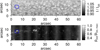 |
Fig. 1 Upperpanel: continuum intensity (normalized to the average value over the field-of-view) of the scan used in this paper. Lower panel: total polarization normalized to its maximum. Scan direction is from bottom to top. The horizontal axis corresponds to the direction of the slit. The blue rectangle marks the area analyzed in this paper, also seen in Fig. 4 (top panel). |
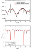 |
Fig. 2 Continuum calibration using a comparison between the FTS spectrum and the measured spectrum. The top panel shows the residual spectrum (black) and the lowpass filtered curve used for the calibration (red). In the bottom panel we compare the degraded FTS spectrum (red) with the calibrated spectrum (black). Δ λ = 0 refers to theFe I 15 648.5 Å spectral line in Table 1. |
3 Verifying data calibration
We note that dividing all observed Stokes I spectra by the empirically determined Fourier-filtered curve as described in Sect. 2 can alter the actual shape of the spectral lines. In particular, small (≈1%) changes in line-depth and line-width may appear. The same problem would arise if the spectral PSF employed is not accurate. Consequently the temperature dependence with optical depth inferred from the inversions (see Sect. 5) could beunrealistic. To make sure that this is not the case, in this section we perform a series of inversions using the SIR code (Stokes Inversion based on Response functions; Ruiz Cobo & del Toro Iniesta 1992) to fit the average Stokes I after applying thenormalization curve and employing the spectral PSF described above. This inversion yields the temperature stratification T(log τ5) of the average quiet Sun, where τ5 indicates the continuum optical depth evaluated at a reference wavelength of 5000 Å. As such, the retrieved T(log τ5) should be similar to the temperature stratification of the quiet Sun. The top panel in Fig. 3 shows the average quiet Sun Stokes I signal (black) and best-fit profiles obtained with the SIR code with one (red), two (blue) and five (green) nodes in temperature. The nodes define the number of optical depth locations log (τ5) where the temperature is modified at each iteration step during the inversion. They correspond, therefore, to the number of degrees of freedom allowed during the inversion. Different nodes are employed because the normalization procedure described above introduces changes in the intensity profiles that vary across wavelength, thereby potentially introducing errors in theretrieved temperature at different optical depths. The bottom panel displays the temperature stratification T(log τ5) inferred by the SIR code with these nodes, along with the temperature from three commonly used semi-empirical quiet Sun models: the Harvard Smithsonian Reference Atmosphere (HSRA; Gingerich et al. 1971) (solid black), the Holwerger-Müller model (HOLMU; Holweger & Mueller 1974) (dashed black), and the VALC model (Vernazza et al. 1981) (dotted black). As Fig. 3demonstrates, the inferred temperatures resemble that of quiet Sun models, thus indicating that our continuum normalization and spectral PSF are adequate, or at the very least we do not introduce uncertainties in the temperature larger than those already existing between semi-empirical models of the quiet Sun. Differences for log τ5 < −2 can be safely ignored since these spectral lines have very little sensitivity above this region (see Sect. 5 and Fig. 7).
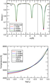 |
Fig. 3 Calibration verification. All curves refer to the mean quiet Sun spectrum. Top panel: observed Stokes I (black) and best-fit profiles obtained with the SIR code and a varying number of nodes (red − 1−, blue − 2− and green −5−). Bottom panel: temperature stratification from the HSRA, VALC and HOLMU (black solid, dotted, and dashed lines, respectively). The color-code is the temperature inferred by the application of the SIR inversion code using a varying number of nodes as in the top panel. |
4 Data analysis
4.1 Region of interest
We used the Stokes V signal of the Fe I at 15 648 Å to identify three-lobed Stokes V profiles. Multi-lobed circular polarization profiles appear predominantly in this spectral line because it possesses the largest Landé factor of all the lines included in the observed wavelength range (see Table 1). The blue rectangle in Fig. 1 shows the position of a large patch containing three-lobed Stokes V profiles. The top panel in Fig. 4 shows a close-up of this region. An example of the observed circular polarization is given on the bottom panel of this figure. We note that, although the polarization levels are small (0.4–0.6 % in units of the quiet Sun continuum intensity), in this example the lobes are about ten times above the noise level (indicated by the shaded area on the bottom panel). Of course, three-lobed Stokes V are not always as clear as in this example. For comparison purposes we provide in Figs. A.1–A.4 a sample of the profiles contained within the blue rectangle. In any case, the signals enclosed by the red contour in Fig. 4 (top panel) are such that all three lobes in Stokes V of the Fe I 15 648 Å spectral line are always above three times the noise level. In Sect. 5 we analyze this region in more detail.
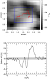 |
Fig. 4 Toppanel: continuum intensity close-up of the analyzed region. See Fig. 1for the full field-of-view. The red and blue contours encircle pixels that were selected for further analysis. Bottom panel: representative three-lobed circular polarization profile of the Fe I 15 468 Å. The black line corresponds to a single pixel. The gray area shows the noise level of 4.5 × 10⁻⁴. |
4.2 Spectral analysis
Before proceeding with the inversion of Stokes profiles, it is worthwhile learning as much as possible from the data by performing a qualitative analysis of the observations. This gives us information about the possible values that the physical parameters might adopt.
Magnetic field strength
In the strong field regime (e.g., Stix 2004, Eq. (3.55)) we can calculate the magnetic field strength B with:
 (1)
(1)
where λ is expressed in Å and B is in Gauss. The above formula gives the line separation between the left and right lobes of the Stokes V profile Δ λ = 2(λ − λ0). Therefore:
 (2)
(2)
The separation of the two lobes of the Stokes V profile is roughly 1 Å (see the bottom panel in Fig. 4), corresponding to a magnetic field strength of about 1500 G. This gives us a rough estimation for the magnetic field strength we can expect to be present in the selected region. Interestingly, with such large values for the magnetic field, one would expect the amplitude of Stokes V to be much larger than 1% and for Stokes I to show some signatures of the Zeeman pattern. However none of these are observed. It is therefore plausible that only a small portion of the plasma harbors such a strong magnetic field. This magnetized region could occupy either a thin vertical layer or a small horizontal and still unresolved fraction of the resolution element.
Temperature gradient
The small observed circular polarization amplitude could also be caused by a temperature stratification varying very slowly with optical depth (i.e., shallow temperature gradient). However, if this were the case, Stokes I would also be very shallow, which is at odds with the fact that the line-core intensity in Stokes I is not very different from the line-core intensity of the average quiet Sun. For instance, the line-core intensity for Fe I 15 648 Å is about 0.77 in the selected region (see top-left panels in Figs. 5 and 6) and 0.74 in the average quiet Sun profile (bottom panel in Fig. 2 or top panel in Fig. 3). The discrepancy between Stokes I and V could be explained if, again, we invoke the presence of unresolved structure (either vertically or horizontally) within the resolution element, where some region of the solar photosphere would have a very shallow temperature gradient and strong magnetic field.
Inclination of the magnetic field
As can be seen in Figs. 5 and 6 and also in Figs. A.1–A.4, Stokes Q and U are always below the noise level. In these NIR spectral lines, this indicates that the magnetic field is close to being aligned with the observer’s line-of-sight (Martínez González et al. 2008). It is also possible that the field lines are arranged in a way that Q and U cancel themselves out.
Velocity
The Stokes V signal is not centered at the same wavelength position as the Stokes I signal (see for instance Figs. 5 and 6). This reinforces the idea of a complex atmosphere with vastly different physical properties either stacked up vertically or lying next to each other.
The separation of the two negative polarity lobes in the blue wing of the Stokes V signal is roughly 500 mÅ (see bottom panel in Fig. 4). This corresponds to a velocity difference of about 9 km s−1. While the separation is most likely due to magnetic field strength, it gives an upper limit of possible velocity difference in the observed region.
Unresolved structure and Stokes V area asymmetry
We have already gathered evidence pointing towards the existence of variations in the physical parameters within the resolution element. The question that arises next is whether these variations occur predominantly along the ray-path (i.e., line-of-sight) or perpendicularly to it. In the former case we speak about variations of the physical parameters with the optical depth τ5, whereas in the latter case we refer to horizontal variations within the resolution element or horizontally unresolved structure. The area asymmetry, δa, in the circular polarization is a very useful tool that can be employed to distinguish between these two limiting cases. It is defined as the integral over wavelength of the Stokes V signal normalized to its total area:
 (3)
(3)
As demonstrated by Landolfi & Landi Degl’Innocenti (1996) a sufficient and necessary condition for δa≠ 0 is the presence of a gradient in the line-of-sight velocity with optical depth (d vlos∕dτ5≠0). The introduction of gradients in other physical quantities such as the magnetic field strength B or the inclination of the magnetic field with respect to the line-of-sight γ increases the absolute value of δa of the observed Stokes V signal (Sanchez Almeida & Lites 1992; Solanki & Montavon 1993).
Most of the observed Stokes V signals that we are analyzing (see e.g., bottom panel in Fig. 4) have low area asymmetries δa < 0.1 (with an average absolute value of  ). Usually this is taken as an indication that the three-lobe structure in the circular polarization is not due to variations of the velocity andmagnetic field with optical depth, but instead produced by the presence of horizontally unresolved components within the resolution element. However, as demonstrated by (Borrero et al. 2004; see their Fig. 8) the NIR spectral lines employed in this work show small amounts of area asymmetry even in the presence of large gradients along the line-of-sight in the physical parameters. Because of this we cannot rule out the existence of such variations. Consequently, we must study these two cases separately.
5 Stokes inversion set up
We used the SIR code (Ruiz Cobo & del Toro Iniesta 1992) to simultaneously invert the Stokes profiles of the Fe I spectral lines at 15 648 Å, 15 652 Å, and 15 662 Å (see Table 1). Details about inversion codes for the radiative transfer equation applied to polarized light can be found in the recent review by del Toro Iniesta & Ruiz Cobo (2016). Of particular interest is the concept of nodes, which are locations in the optical depth scale where the derivatives of the Stokes vector with respect to the physical parameters are evaluated (see Sect. 7.2 of the aforementioned review). These derivatives are used by the minimization algorithm to perturb the physical parameters at each iteration step so as to improve the χ2 merit-function between the observed and theoretical Stokes parameters (del Toro Iniesta & Ruiz Cobo 2016, Eq. (35)). The total number of nodes during the inversion equals the number of free parameters.
During the minimization of the χ2 merit-function, some Stokes parameters can be given more priority than others by changing the weights that each of them have in the calculation of χ2. In the present work our goal is to fit all four measured Stokes profiles reasonably well, with a particular emphasis on capturing the three-lobed feature observed in the Fe I 15 648 Å line. Therefore Stokes V is weighted above the other Stokes parameters (I, Q and U). More details are given below.
Before proceeding with the inversion of the entire region of interest (see blue square in the top panel of Fig. 4) we tested our inversions on a single pixel, inside this region, where the three-lobed Stokes V is very prominent, and made sure that the selected weights produce good fits to the observations. In addition to this, the inversion of each pixel was repeated 50 times with different random initializations (see Borrero et al. 2017). The result with the best χ2 from those 50 inversions was then selected for that particular pixel. This was done in order to prevent the Levenberg-Marquardt inversion algorithm (Press et al. 1986) from falling into any local minimum in the χ2 -hypersurface. We note that the highest atmospheric layer in our atmospheric models is log τ5 = −3 so as to avoid having nodes in regions of low sensitivity to the various physical parameters (see Sect. 6 for more details).
In orderto fit the multi-lobe structure of the circular polarization signals, variations in the velocity and magnetic field must be included and permitted during the inversion. Unfortunately (see Sect. 4.2) the study of the area asymmetry did not allow usto disentangle the presence of vertical or horizontal variations. Therefore we study both possibilities independently.
5.1 One-component inversion
Here we assume that the entire resolution element is filled with one single component where the physical parameters vary with optical depth. During the inversion we found that the SIR code could not fit all four Stokes parameters simultaneously while reproducing the three-lobed pattern in Stokes V. This happened even when increasing the weight given to Stokes V. Because of this we split the inversion in two different stages. In the first stage only Stokes I and V were inverted: weights to Q and U were set to zero and Stokes V was given 20 times more weight than Stokes I. The temperatureT(τ5), magnetic field strength B(τ5), inclination of the magnetic field with respect to the observer’s line-of-sight γ(τ5), and line-of-sight velocity vlos(τ5) were allowed to change in three nodes each. Microturbulence was allowed to change with one node. The azimuth in this first step was not allowed to change and was kept at zero.
Subsequently, a second inversion stage was performed using the results from the previous stage for initialization and now including Q and U, which were given the same weight as Stokes I (20 times less than Stokes V). All physical parameters were kept the same as the results from the first stage, except for the azimuth of the magnetic field in the plane perpendicular to the line-of-sight ϕ(τ5) which was allowed to change in two nodes.
Combining both stages the total number of free parameters employed was 15. This procedure allowed us to fit reasonably well the polarized Stokes parameters (Q, U, and V) including the three-lobed structure in the circular polarization (see Fig. 5). Owing to the smaller weight given to Stokes I during the inversion, the fits in Stokes I are of lesser quality than those of Stokes V. Moreover, as can be seen in this figure, the depth of Stokes I for the Fe I spectral line at 15 662 Å (i.e., third line from the right in Figs. 5, 6) is particularly poorly reproduced. This could be due to the oscillator strength employed for this line not being as accurate as the others (see Table 1). We note that the presence of telluric and molecular blends, interference fringes, assumption of LS coupling, and so on, make the intensity profiles of these lines in the NIR notoriously difficult to fit4.
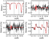 |
Fig. 5 Representative pixel for one-component fit. The black curve shows the observed Stokes profiles: I (top-left), Q (top-right), U (bottom-left), and V (bottom-right). The red curve shows the best-fit profiles obtained from the inversion (i.e., smallest χ2). |
5.2 Two-component inversion
In the two-component inversion we assume that the resolution element is composed of two distinct atmospheric components that are interlaced horizontally. The first one covers a fraction of the total area of the resolution element α. The area occupied by the second component would therefore be (1–α). In order to clearly separate the inversions in this section from the previous ones we take the magnetic and kinematic parameters to be constant with optical depth in both components. In this fashion the three-lobed structure of the observed circular polarization profiles (see bottom panel in Fig. 4) is completely ascribed to the horizontal variations (i.e., differences between the first and second components) of the physical parameters as opposed to the vertical variations of the one-component inversions (Sect. 5.1). We note that the temperature in both components must be dependent on τ5 otherwise Planck’s function would be the same at all photospheric layers and there would be no spectral features (i.e., no absorption in Stokes I and only a flat continuum).
During the inversion, the temperature T for each component was allowed to change in three nodes, while for B, vlos and microturbulence we employed only one node (i.e., constant values with τ5) per component. Together with the filling factor α this adds up to a total of 13 free parameters during the inversion. For reasons that will become apparent later, the magnetic field inclination was fixed and not allowed to change during the inversion to γ = 0° for the first component (constant with τ5) and γ = 180° for the second component. Just as before, the weight of Stokes V was 20 times larger than for Stokes I. Since the inclination of the magnetic field is such that the magnetic field is always aligned with the observer’s line-of-sight (parallel for γ = 0° and antiparallel for γ = 180°) this set-up does not produce any linear polarization and therefore the weights for Stokes Q and U were set to zero. Unlike the one-component inversion in the previous section here the inversion was performed in a single stage.
The fit to the observed Stokes profiles achieved with the aforementioned configuration is of similar quality to the one-component inversion. An example can be seen in Fig. 6. Owing to the fact that we have twice as many free parameters in the temperature than in the one-component inversion, the quality of the fits to Stokes I has increased.
6 Stokes inversion results
Figure 7 displays a measure of the sensitivity to the physical parameters for the spectral lines in Table 1. It was obtained by adding up the individual unsigned response functions of the four Stokes parameters using the weights employed during the inversion (see Sect. 5), integrating in wavelength and normalizing the resulting curve to have an area equal to one. The model employed to calculate these response functions is the average model from the two-component inversion (see Sects. 5.1 and 6.1). The resulting functions show that the NIR lines discussed in this paper form deep in the solar photosphere, in particular when compared to the commonly used Fe I spectral lines in the visible (see also Borrero et al. 2016). While our models reach up to log τ5 = −3 (see Sect. 5), most of the sensitivity of the spectral lines used in this work comes from a thin photospheric layer located between logτ5 ∈ [−2, 0.5]. The temperature is sensitive to slightly deeper layers compared to the other atmospheric parameters. Outside this range the response functions are too small and therefore the uncertainty in the inference of the physical parameters increases. Because of this, in the following we only discuss the inversion results obtained in the range log τ5 ∈ [−2, 0.5].
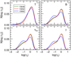 |
Fig. 7 Response functions integrated over wavelength, added up for all four Stokes parameters and plotted as a function of the logarithm of the optical depth log τ5. Top-left: response to the temperature T. Top-right: response to the line-of-sight velocity vlos. Bottom-left: response to the magnetic field strength B. Bottom-right: response to the inclination of the magnetic field with respect to the observer’s line-of-sight γ. Different colors correspond to different spectral lines. Green: 15 648 Å, red: 15 652 Å, blue: 15 662 Å. The response functions are calculated with the atmosphere resulting from the two-component inversion shown in Fig. 6. |
6.1 One-component result
The inferred physical parameters as a function of optical depth from the one component inversion (Sect. 5.1) are presented in Fig. 8. The results for the individual pixels within the region of interest within the red contour in Fig. 4 (top panel) are indicated by the black lines. We find that the temperature in the range log τ5 ∈ [−2, 0.5] closely follows that of the HSRA atmosphere (red line in the top-left panel). The magnetic field (top-right panel) quickly decreases from kilo-Gauss values in the deep photosphere (log τ5 ≈ 0) to almost zero approximately 150–200 kmhigher up (logτ5 ≈−1.5). The photospheric layer with large magnetic fields possesses redshifted velocities that turn into blueshifts as the magnetic field decreases higher up. In both cases, the absolute velocities are about 1–2 km s−1 (bottom-left panel). It must be borne in mind that a change of sign in vlos can be due solely to projection effects (i.e., observer’s line-of-sight).
The magnetic field is highly inclined with respect to the observer (γ ≈ 90°; bottom-right panel) at all optical depths. At closer inspection we see that it points slightly away from the observer in the strong field region (γ(logτ5 ≈ 0) > 90°) and slightly towards the observer higher up in the weak-field region (γ(logτ5 ≈−1.5) < 90°). The change of polarity (with respect to the observer) in the inclination of the magnetic field, as well as the change from blueshifted to redshifted velocities, are key features in reproducing three-lobed circular polarization profiles in the analyzed NIR spectral lines. They have previously been reported in other solar regions, such as sunspot penumbrae (see Fig. 3 in Borrero et al. 2004). To demonstrate the need for a polarity change we have conducted two experiments. In the first one we made γ = 90° whenever γ > 90° in Fig. 8 while keeping all other physical parameters the same, and using the resulting atmospheric model to create synthetic profiles of the observed spectral lines. In the second one we did the opposite, that is, we kept γ = 90° whenever γ < 90° while keeping all other physical parameters the same. In both cases, the polarity change is effectively removed. Interestingly, in both instances, the third lobe in Stokes V of the Fe I 15 648.5 Å immediately disappears, thereby proving that the change in polarity is a necessary feature.
It is important to mention here that, at each iteration step, the SIR inversion code performs a smooth interpolation in τ5 of the physical parameters between the values at the nodes. As a consequence, if the code finds it necessary to change from γ < 90° to γ > 90° (i.e., polarity change) to fit the multi-lobe structure of Stokes V, it follows then that γ ≈ 90° somewhere in the optical depth region where the line is formed. Such a highly inclined magnetic field will produce a strong linear polarization signal. However, the observed Q and U profiles are below the noise level (see black lines in Fig. 5). The inversion code is therefore compelled to reduce the amount of linear polarization by including large changes with optical depth in the azimuth of the magnetic field ϕ. These large variations are displayed in Fig. 9. Here we can see that ϕ changes by about 2000 degreesbetween logτ5 ∈ [−2, 0.5]. If real, this would imply that over a vertical distance of 200–300 km, the magnetic field performs about four to five full rotations on the plane perpendicular to the observer’s lines-of-sight.
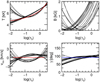 |
Fig. 8 Results as a function of the logarithm of the optical depth (logτ5) for the one component inversion: temperature T (top-left), magnetic field strength B (top-right), line-of-sight velocity vlos (bottom-left), inclination of the magnetic field with respect to the observer’s line-of-sight γ (bottom-right). Individual black curves correspond to the inversion of individual pixels. The red curve on the top-left panels shows the temperature stratification from the HSRA model. Red/blue curves on the lower panels indicate vlos = 0 (bottom-left)and γ = 90° (i.e., horizontal magnetic field; bottom-right). |
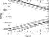 |
Fig. 9 Azimuth of the magnetic field in the plane perpendicular to the observer’s line of sight ϕ as a functionof the logarithm of the optical depth logτ5 for the one-component inversion. Individual black curves correspond to the inversion of individual pixels. The average gradient is 700° per optical depth scale decade, indicating multiple rotations of the magnetic field vector within the photosphere. |
6.2 Two-component result
Figure 10 shows the inferred physical parameters as a function of the optical depth from the two-component inversion (Sect. 5.2). Red curves represent the results for each of the inverted pixels in the region with the red contour in Fig. 4 (Top panel) for the first of the two components. This first component features a hot plasma with a shallow temperature gradient (top-left panel), a strong magnetic field (B ≳ 1000; top-right panel), and redshifted velocities of about 1.5 km s−1 (bottom-leftpanel). Likewise, the blue curves represent the physical parameters for the second component. Here, the temperature is colder, at logτ5 = 0, by about 1000 K than in the first component. This temperature difference increases towards higher layers and reaches about 3000 K at log τ5 = −2. The magnetic field in this component is much weaker and very close to zero (B ≈ 10) and the line-of-sight velocities are blueshifted by about 0.6 km s−1. By construction (see Sect. 5.2) the magnetic field is always vertical in both components, but it points away from (γ = 180°) and towards (γ = 0°) the observer in the hot and cold components, respectively. We note that it was not possible to fit the third lobe in Stokes V if both components had the same polarity5. An azimuth of the magnetic field was not determined since the magnetic field vector is parallel to the line-of-sight. The filling factor of the first component (i.e., strong field component) is within α ∈ [0.2, 0.4] for most pixels.
One could be tempted to argue that the magnetic field in the second component, being so low, is indeed zero or at least negligible. However, as we demonstrate in Fig. 11 (upper panel) a B ≥ 0 in the second component is absolutely necessary if the three-lobed structure in the circular polarization is to be reproduced. This figure shows the Stokes V profiles of the spectral line Fe I 15 648 Å created by the first and second components in red and blue colors, respectively. The black line corresponds to the final Stokes V resulting from combining the previous two with a filling factor for the first component of α =0.27. Due to its larger magnetic field, the level of circular polarization created by the first component is larger than that of the second one, and in spite of its shallower temperature decrease with optical depth. However, the amount of Stokes V generated by the second component becomes comparable to that of the first component once we consider that the latter occupies a smaller fraction of the resolution element (0.73 vs. 0.27). When comparing the Stokes I profiles emerging from each ofthe two components individually (lower panel in Fig. 11) we see that the first component, being much hotter at τ5 = 1 than the average quiet Sun, produces a continuum intensity of 1.1 (red), whereas the second component, having a similar temperature at τ5 = 1 to that of the average quiet Sun, produces also a similar continuum intensity of 0.97 (blue). Once both components are added, considering a filling factor of α = 0.27 for the first component, the resulting continuum intensity is very close to 1.0 (as observed in Figs. 5 and 6).
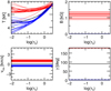 |
Fig. 10 As in Fig. 8 but for the two-component inversion. Red and blue colors represent the first and second components, respectively. Each curve corresponds to a single pixel. |
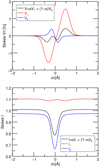 |
Fig. 11 Comparison of synthetic Stokes V (upper panel) and I (lower panel) profiles of Fe I 15 648 Å in a two-component atmosphere. The black curve is the inversion result presented in Fig. 6. The red (blue) profile is caused by only the first (second) component, respectively. The respective magnetic field strengths are B = 1147 G and B = 9 G and the filling factor of the component with the strong magnetic field is α = 0.27. We note that both components produce circular polarization signals of similar amplitudes in spite of the very different magnetic fields. The final continuum intensity (lower panel) is about 1.0 (normalized to the quiet Sun value) in spite of the first component featuring very high temperatures (see red lines in the upper-left panel of Fig. 10). |
7 Discussion
Despite the very different geometrical configurations employed (Sect. 5), the one- and two-component inversions yield physical parameters that are largely consistent with each other. In both cases, we detect, within the resolution element, regions of the photosphere harboring a strong magnetic field (B ≥ 1000 G), that point away from the observer (γ > 90°), and where the velocity is redshifted (vlos > 0). Along with this, we find other regions within the resolution element with a much weaker magnetic field (B ≈ 10 G), that points towards the observer (γ < 90°), and where the velocity is blueshifted (vlos < 0). In particular, the physical parameters at logτ5 ≈ 0 inferred from the one-component inversions (Fig. 8) are very similar to those of the first component in the two-component inversion (red curves in Fig. 10). Likewise, the physical parameters at log τ5 ≈−1.5 inferred from the one-component inversions (Fig. 8) are very similar to those of the second component in the two-component inversion (blue curves in Fig. 10).
It is notpossible at this stage to say whether these two regions are interlaced horizontally (i.e., lying next to each other) or vertically (i.e., lying one on top of the other). The latter case is represented by the one-component inversion, whereas the former case is represented by the two-component inversion. On the one hand we cannot employ the quality of the fits in order to decide which type of inversion is to be preferred because both reproduce reasonably well the observed Stokes profiles (cf. Fig. 5 and Fig. 6; see also Fig. A.1 through Fig. A.4). On the other hand, the area asymmetry in these NIR spectral lines (Table 1) is small even in the presence of very strong gradients along the line-of-sight in the magnetic and kinematic parameters Borrero et al. (2004), and therefore cannot be invoked to decide which inversion is to be preferred (see Sect. 4.2). More complex inversion approaches, in particular multi-component inversions with gradients, could also be used to reproduce the observed signal. Since this would significantly increase the number of free parameters, we limit ouranalysis to inversions with the least possible number of degrees of freedom that still fit the Stokes V profile.
An alternative approach to decide between the one- and two-component inversion is to look at the realism (or lack of) of the inferred physical parameters. As mentioned in Sect. 6.1, the one-component inversion leads to the magnetic field performing several rotations (see Fig. 9) in the plane perpendicular to the observer’s line-of-sight along a vertical distance of 200–300 km. We cannot readily regard this result as unphysical because similar configurations have been previously reported for the velocity (Bonet et al. 2010; Wedemeyer-Böhm et al. 2012). In particular, the latter authors find that, in three-dimensional MHD simulations performed with the CO5BOLD code, the velocity vector can perform many rotations over such a short vertical distance (see their Fig. 3). In our observations we find that the magnetic field could also behave in this fashion. On the other hand, these rotations could be simply an artifact of the SIR inversion code attempting to fit three-lobed Stokes V profiles while keeping Q and U close to zero using smooth variations with τ5 in the physical parameters. As discussed in Sect. 6.1 this forces the code to find a solution where the magnetic field changes polarity (γ < 90° → γ > 90°), thus becoming horizontal with respect to the observer in the middle of the line-forming region (γ(logτ5 ≈−1) = 90°). The large variations in the azimuthal angle ϕ appear then as a consequence of the requirement to make the linear polarization signals vanish in spite of the horizontal magnetic field. It must be borne in mind that it might be possible to fit the profiles if we include a discontinuity in γ at around logτ5 = −1, with γ = 0° above and γ = 180° below. Such a configuration would still feature a polarity change, thereby fitting the three-lobed Stokes V profiles, but with a magnetic field that is always aligned with the observer’s line-of-sight (i.e., either parallel or antiparallel to it) which produces, as observed, no linear polarization. In this case there would be no need for any variations of the azimuthal angle ϕ with optical depth.
Some results from the two-component inversion could also be questioned. In particular some doubts could be cast on the temperature stratification T(logτ5) of the strong field component (see red curves on the top-left panel of Fig. 10). Such an atmospheric component is hotter than the quiet Sun (black curves in this figure shows the HSRA model) by 1000–3000 K, and it decays very slowly towards higher photospheric layers. While seemingly unrealistic, similar temperature stratifications have previously been reported in unipolar magnetic elements in the quiet Sun (Lagg et al. 2010). Moreover, regions with multi-lobe Stokes V profiles in the Fe I spectral lines at 6300 Å were analyzed by Quintero Noda et al. (2014b) who also found enhanced temperatures, kilo-Gauss magnetic fields, and large redshifted line-of-sight velocities. These properties are somewhat similar to the ones inferred for the strong field component in our two-component inversion. Therefore, the inferred temperatures cannot be considered as unrealistic and cannot be used to rule out the results from the two-component inversion.
8 Conclusions and future work
We have analyzed high-quality (i.e., polarimetric noise below 5 × 10⁻⁴ in units of the quiet Sun intensity) and high-spatial-resolution (≈0.4′′) spectropolarimetric data (full Stokes vector) from the quiet Sun recorded with the GRIS instrument attached to the 1.5-m German solar telescope GREGOR. The observed spectral region includes three Fe I lines located in the NIR (15 650 Å) that are highly sensitive to the magnetic field. We focus on a small region (≈ 0.5′′ in diameter) in the quiet Sun where the circular polarization profiles of one of those lines presents three lobes. This feature is indicative of variations in the physical parameters, in particular in the magnetic field and line-of-sight velocity, within the resolution element. To investigate whether those variations occur predominantly along the line-of-sight or perpendicular to it we have performed two kinds of inversion of the observed profiles. In the first one we assume thatthe resolution element is occupied by one magnetic atmosphere where the kinematic and magnetic parameters vary with optical depth (i.e., line-of-sight). In the second one we assume the resolution element to be occupied by two magnetic atmospheres where the kinematic and magnetic parameters are constant with optical depth.
The analysis of the data using both inversion set-ups reveals that the three lobes seen in Stokes V are produced by the presence of magnetic fields of opposite polarity. One of them possesses a strong magnetic field (B ≥ 1000 G) and harbors plasma velocities directed away from the observer, whereas the other one possesses a much weaker field (B ≈ 10 G) where the velocity is directed towards the observer. In spite of these similarities, each kind of inversion also presents some peculiarities.
The one-component inversion fits the observed profiles by invoking large variations in the azimuth of the magnetic field (i.e., rotations of the magnetic field vector in the plane perpendicular to the observer’s line-of-sight). Such swirling or tornado-like configuration has already been found in the velocity (Bonet et al. 2010; Wedemeyer-Böhm et al. 2012). In our work we find that the magnetic field could behave similarly. We emphasize that it could also be possible to fit the observed profiles without such large variations in the azimuth of the magnetic field if we consider discontinuities in the inclination of the magnetic field with respect to the observer’s line-of-sight.
The two-component inversion infers a temperature stratification T(logτ5) in the region with a strong magnetic field that is (much) hotter than the average quiet Sun by 1000–3000 K. High temperatures have been found in magnetic elements (network, Lagg et al. 2010), in strongly magnetized upflow regions inside granules (Borrero et al. 2013) and downflow regions (Quintero Noda et al. 2014b).
Therefore, neither the physical realism nor the goodness of the fits to the observations can be invoked to give preference to one inversion set-up over the other. To answer this question it would be desirable to employ inversion codes for the radiative transfer equation that allow for discontinuities in the physical parameters (Louis et al. 2009; Sainz Dalda et al. 2012; Martínez González et al. 2012; Shaltout & Ichimoto 2015). It would also be appropriate to study whether the Stokes profiles emerging from numerical simulations show a similar behavior, so as to find out the stratification of the physical parameters in those simulations and compare them to the inferred stratifications from the observations (Danilovic et al. 2015).
To resolve the ambiguity discussed in this work, studies of multiple events, possibly with higher spatial resolution will be necessary. The next generation of large solar telescopes, such as DKIST (Rimmele et al. 2015), will provide the high-resolution data needed to advance the study of small scale, complex magnetic features.
Acknowledgements
The 1.5-m GREGOR solar telescope was built by a German consortium under the leadership of the Kiepenheuer-Institut für Sonnenphysik in Freiburg with the Leibniz-Institut für Astrophysik Potsdam, the Institut für Astrophysik Göttingen, and the Max-Planck-Institut für Sonnensystemforschung in Göttingen as partners, and with contributions by the Instituto de Astrofísica de Canarias and the Astronomical Institute of the Academy of Sciences of the Czech Republic.
Appendix
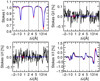 |
Fig. A.1 First example of observed (black), fitted with the one-component inversion (red; Sects. 5.1, 6.1), and with the two-component inversion (blue; Sects. 5.2, 6.2), Stokes profiles in a pixel of the red contour in Fig. 4. |
Inversion results of selected pixels with the red contour in Fig. 4. The black curves show the measured Stokes profiles, while the red/blue curves show the inversion results for the one/two component inversion, respectively.
References
- Anstee, S. D., & O’Mara, B. J. 1995, MNRAS, 276, 859 [NASA ADS] [CrossRef] [Google Scholar]
- Auer, L. H., & Heasley, J. N. 1978, A&A, 64, 67 [NASA ADS] [Google Scholar]
- Barklem, P. S., & O’Mara, B. J. 1997, MNRAS, 290, 102 [Google Scholar]
- Barklem, P. S., O’Mara, B. J., & Ross, J. E. 1998, MNRAS, 296, 1057 [Google Scholar]
- Bellot Rubio, L. R., Collados, M., Ruiz Cobo, B., & Rodríguez Hidalgo I. 2000a, ApJ, 534, 989 [NASA ADS] [CrossRef] [Google Scholar]
- Bellot Rubio, L. R., Ruiz Cobo, B., & Collados, M. 2000b, ApJ, 535, 489 [NASA ADS] [CrossRef] [Google Scholar]
- Bellot Rubio, L. R., Rodríguez Hidalgo, I., Collados, M., Khomenko, E., & Ruiz Cobo B. 2001, ApJ, 560, 1010 [NASA ADS] [CrossRef] [Google Scholar]
- Bellot Rubio, L. R., Balthasar, H., & Collados, M. 2004, A&A, 427, 319 [NASA ADS] [CrossRef] [EDP Sciences] [Google Scholar]
- Berkefeld, T., Schmidt, D., Soltau, D., von der Lühe, O., & Heidecke, F. 2012, Astron. Nachr., 333, 863 [NASA ADS] [CrossRef] [Google Scholar]
- Bloomfield, D. S., Solanki, S. K., Lagg, A., Borrero, J. M., & Cally, P. S. 2007, A&A, 469, 1155 [NASA ADS] [CrossRef] [EDP Sciences] [Google Scholar]
- Bonet, J. A., Márquez, I., Sánchez Almeida, J., et al. 2010, ApJ, 723, L139 [NASA ADS] [CrossRef] [Google Scholar]
- Borrero, J. M., & Solanki, S. K. 2010, ApJ, 709, 349 [NASA ADS] [CrossRef] [Google Scholar]
- Borrero, J. M., Bellot Rubio, L. R., Barklem, P. S., & del Toro Iniesta J. C. 2003, A&A, 404, 749 [NASA ADS] [CrossRef] [EDP Sciences] [Google Scholar]
- Borrero, J. M., Solanki, S. K., Bellot Rubio, L. R., Lagg, A., & Mathew, S. K. 2004, A&A, 422, 1093 [NASA ADS] [CrossRef] [EDP Sciences] [Google Scholar]
- Borrero, J. M., Lagg, A., Solanki, S. K., & Collados, M. 2005, A&A, 436, 333 [NASA ADS] [CrossRef] [EDP Sciences] [Google Scholar]
- Borrero, J. M., Solanki, S. K., Lagg, A., Socas-Navarro, H., & Lites, B. 2006, A&A, 450, 383 [NASA ADS] [CrossRef] [EDP Sciences] [Google Scholar]
- Borrero, J. M., Bellot Rubio, L. R., & Müller, D. A. N. 2007, ApJ, 666, L133 [NASA ADS] [CrossRef] [Google Scholar]
- Borrero, J. M., Martínez-Pillet, V., Schlichenmaier, R., et al. 2010, ApJ, 723, L144 [NASA ADS] [CrossRef] [Google Scholar]
- Borrero, J. M., Martínez Pillet, V., Schmidt, W., et al. 2013, ApJ, 768, 69 [NASA ADS] [CrossRef] [Google Scholar]
- Borrero, J. M., Asensio Ramos, A., Collados, M., et al. 2016, A&A, 596, A2 [NASA ADS] [CrossRef] [EDP Sciences] [Google Scholar]
- Borrero, J. M., Franz, M., Schlichenmaier, R., Collados, M., & Asensio Ramos A. 2017, A&A, 601, L8 [NASA ADS] [CrossRef] [EDP Sciences] [Google Scholar]
- Cabrera Solana, D., Bellot Rubio, L. R., Borrero, J. M., & Del Toro Iniesta J. C. 2008, A&A, 477, 273 [NASA ADS] [CrossRef] [EDP Sciences] [Google Scholar]
- Chandrasekhar, S., & Breen, F. H. 1946, ApJ, 104, 430 [NASA ADS] [CrossRef] [Google Scholar]
- Collados, M., López, R., Páez, E., et al. 2012, Astron. Nachr., 333, 872 [NASA ADS] [CrossRef] [Google Scholar]
- Danilovic, S., Cameron, R. H., & Solanki, S. K. 2015, A&A, 574, A28 [NASA ADS] [CrossRef] [EDP Sciences] [Google Scholar]
- del Toro Iniesta, J. C. & Ruiz Cobo B. 2016, Liv. Rev. Solar Phys., 13, 4 [Google Scholar]
- del Toro Iniesta, J. C., Bellot Rubio, L. R., & Collados, M. 2001, ApJ, 549, L139 [NASA ADS] [CrossRef] [Google Scholar]
- Franz, M., & Schlichenmaier, R. 2013, A&A, 550, A97 [NASA ADS] [CrossRef] [EDP Sciences] [Google Scholar]
- Franz, M., Collados, M., Bethge, C., et al. 2016, A&A, 596, A4 [NASA ADS] [CrossRef] [EDP Sciences] [Google Scholar]
- Gingerich, O., Noyes, R. W., Kalkofen, W., & Cuny, Y. 1971, Sol. Phys., 18, 347 [NASA ADS] [CrossRef] [Google Scholar]
- Holweger, H., & Mueller, E. A. 1974, Sol. Phys., 39, 19 [NASA ADS] [CrossRef] [Google Scholar]
- Ichimoto, K., Shine, R. A., Lites, B., et al. 2007, PASJ, 59, S593 [NASA ADS] [Google Scholar]
- Ichimoto, K., Tsuneta, S., Suematsu, Y., et al. 2008, A&A, 481, L9 [NASA ADS] [CrossRef] [EDP Sciences] [Google Scholar]
- Jafarzadeh, S., Rouppe van der Voort, L., & de la Cruz Rodríguez, J. 2015, ApJ, 810, 54 [NASA ADS] [CrossRef] [Google Scholar]
- Khomenko, E. V., Collados, M., Solanki, S. K., Lagg, A., & Trujillo Bueno J. 2003, A&A, 408, 1115 [NASA ADS] [CrossRef] [EDP Sciences] [Google Scholar]
- Lagg, A., Solanki, S. K., Riethmüller, T. L., et al. 2010, ApJ, 723, L164 [NASA ADS] [CrossRef] [Google Scholar]
- Lagg, A., Solanki, S. K., Doerr, H.-P., et al. 2016, A&A, 596, A6 [NASA ADS] [CrossRef] [EDP Sciences] [Google Scholar]
- Landi Degl’Innocenti, E., & Landi Degl’Innocenti M. 1981, Nuovo Cimento B Serie, 62, 1 [NASA ADS] [CrossRef] [Google Scholar]
- Landi Degl’Innocenti, E., & Landolfi, M. 1983, Sol. Phys., 87, 221 [NASA ADS] [Google Scholar]
- Landolfi, M., & Landi Degl’Innocenti E. 1996, Sol. Phys., 164, 191 [NASA ADS] [CrossRef] [Google Scholar]
- Livingston, W., & Wallace, L. 1991, An atlas of the solar spectrum in the infrared from 1850 to 9000 cm-1 (1.1 to 5.4 micrometer) [Google Scholar]
- Louis, R. E., Bellot Rubio, L. R., Mathew, S. K., & Venkatakrishnan, P. 2009, ApJ, 704, L29 [NASA ADS] [CrossRef] [Google Scholar]
- Martínez González, M. J., Asensio Ramos, A., López Ariste, A., & Manso Sainz R. 2008, A&A, 479, 229 [NASA ADS] [CrossRef] [EDP Sciences] [Google Scholar]
- Martínez González, M. J., Bellot Rubio, L. R., Solanki, S. K., et al. 2012, ApJ, 758, L40 [NASA ADS] [CrossRef] [Google Scholar]
- Martínez González, M. J., Pastor Yabar, A., Lagg, A., et al. 2016, A&A, 596, A5 [NASA ADS] [CrossRef] [EDP Sciences] [Google Scholar]
- Martínez Pillet, V., Del Toro Iniesta, J. C., & Quintero Noda C. 2011, A&A, 530, A111 [NASA ADS] [CrossRef] [EDP Sciences] [Google Scholar]
- Müller, D. A. N., Schlichenmaier, R., Steiner, O., & Stix, M. 2002, A&A, 393, 305 [NASA ADS] [CrossRef] [EDP Sciences] [Google Scholar]
- Nave, G., Johansson, S., Learner, R. C. M., Thorne, A. P., & Brault, J. W. 1994, ApJS, 94, 221 [NASA ADS] [CrossRef] [Google Scholar]
- Pozuelo, S. E., Bellot Rubio, L. R., & de la Cruz Rodríguez, J. 2016, ApJ, 832, 170 [NASA ADS] [CrossRef] [Google Scholar]
- Press, W. H., Flannery, B. P., & Teukolsky, S. A. 1986, Numerical recipes. The art of scientific computing (Cambridge: University Press) [Google Scholar]
- Quintero Noda, C., Martínez Pillet, V., Borrero, J. M., & Solanki, S. K. 2013, A&A, 558, A30 [NASA ADS] [CrossRef] [EDP Sciences] [Google Scholar]
- Quintero Noda, C., Borrero, J. M., Orozco Suárez, D., & Ruiz Cobo B. 2014a, A&A, 569, A73 [NASA ADS] [CrossRef] [EDP Sciences] [Google Scholar]
- Quintero Noda, C., Ruiz Cobo, B., & Orozco Suárez D. 2014b, A&A, 566, A139 [NASA ADS] [CrossRef] [EDP Sciences] [Google Scholar]
- Rimmele, T., McMullin, J., Warner, M., et al. 2015, IAU General Assembly, 22, 2255176 [NASA ADS] [Google Scholar]
- Rueedi, I., Solanki, S. K., Keller, C. U., & Frutiger, C. 1998, A&A, 338, 1089 [NASA ADS] [Google Scholar]
- Ruiz Cobo, B., & del Toro Iniesta J. C. 1992, ApJ, 398, 375 [NASA ADS] [CrossRef] [Google Scholar]
- Sainz Dalda, A., Martínez-Sykora, J., Bellot Rubio, L., & Title, A. 2012, ApJ, 748, 38 [NASA ADS] [CrossRef] [Google Scholar]
- Sanchez Almeida, J., & Lites, B. W. 1992, ApJ, 398, 359 [NASA ADS] [CrossRef] [Google Scholar]
- Sanchez Almeida, J., Collados, M., & del Toro Iniesta J. C. 1988, A&A, 201, L37 [NASA ADS] [Google Scholar]
- Sanchez Almeida, J., Collados, M., & del Toro Iniesta J. C. 1989, A&A, 222, 311 [NASA ADS] [Google Scholar]
- Schlichenmaier, R., & Collados, M. 2002, A&A, 381, 668 [NASA ADS] [CrossRef] [EDP Sciences] [Google Scholar]
- Schlichenmaier, R., Müller, D. A. N., Steiner, O., & Stix, M. 2002, A&A, 381, L77 [NASA ADS] [CrossRef] [EDP Sciences] [Google Scholar]
- Schmidt, W., von der Lühe, O., Volkmer, R., et al. 2012, in Second ATST-EAST Meeting: Magnetic Fields from the Photosphere to the Corona., eds. T. R. Rimmele, A. Tritschler, F. Wöger, et al., ASP Conf. Ser., 463, 365 [NASA ADS] [Google Scholar]
- Shaltout, A. M. K., & Ichimoto, K. 2015, PASJ, 67, 27 [NASA ADS] [CrossRef] [Google Scholar]
- Socas-Navarro, H., & Manso Sainz R. 2005, ApJ, 620, L71 [NASA ADS] [CrossRef] [Google Scholar]
- Solanki, S. K., & Montavon, C. A. P. 1993, A&A, 275, 283 [NASA ADS] [Google Scholar]
- Stenflo, J. O., Solanki, S., Harvey, J. W., & Brault, J. W. 1984, A&A, 131, 333 [NASA ADS] [Google Scholar]
- Stix, M. 2004, The sun: an introduction (Berlin Heidelberg: Springer-Verlag) [Google Scholar]
- Vernazza, J. E., Avrett, E. H., & Loeser, R. 1981, ApJS, 45, 635 [NASA ADS] [CrossRef] [Google Scholar]
- Viticchié, B. 2012, ApJ, 747, L36 [NASA ADS] [CrossRef] [Google Scholar]
- Wedemeyer-Böhm, S., Scullion, E., Steiner, O., et al. 2012, Nature, 486, 505 [NASA ADS] [CrossRef] [PubMed] [Google Scholar]
The wavelength calibration is done assuming that the line-core positions of the spectral lines on the average quiet Sun intensity (Stokes I) profiles are located at the laboratory wavelengths in Table 1 and shifted by 395 ms−1, which is the estimated net effect of the convective blueshift and gravitational redshift. This estimation is done with the FTS spectrum.
Publicly available at http://archive.leibniz-kis.de/pub/ gris/
The same PSF is also used during the inversions (Sect. 5).
Poor fits in Stokes I can also seen in Figs. 3–4 in Cabrera Solana et al. (2008), Fig. 1 in Bellot Rubio et al. (2000a), Fig. 2 in del Toro Iniesta et al. (2001), Fig. 6 in Borrero et al. (2016). Some of these works obtained poor fits in spite of employing a depth-dependent (i.e., more than one node) microturbulent velocity.
A single-polarity atmosphere also failed to reproduce the three-lobe Stokes V in the one-component inversion (see Sect. 6.1)
All Tables
All Figures
|
Fig. 1 Upperpanel: continuum intensity (normalized to the average value over the field-of-view) of the scan used in this paper. Lower panel: total polarization normalized to its maximum. Scan direction is from bottom to top. The horizontal axis corresponds to the direction of the slit. The blue rectangle marks the area analyzed in this paper, also seen in Fig. 4 (top panel). |
| In the text | |
|
Fig. 2 Continuum calibration using a comparison between the FTS spectrum and the measured spectrum. The top panel shows the residual spectrum (black) and the lowpass filtered curve used for the calibration (red). In the bottom panel we compare the degraded FTS spectrum (red) with the calibrated spectrum (black). Δ λ = 0 refers to theFe I 15 648.5 Å spectral line in Table 1. |
| In the text | |
|
Fig. 3 Calibration verification. All curves refer to the mean quiet Sun spectrum. Top panel: observed Stokes I (black) and best-fit profiles obtained with the SIR code and a varying number of nodes (red − 1−, blue − 2− and green −5−). Bottom panel: temperature stratification from the HSRA, VALC and HOLMU (black solid, dotted, and dashed lines, respectively). The color-code is the temperature inferred by the application of the SIR inversion code using a varying number of nodes as in the top panel. |
| In the text | |
|
Fig. 4 Toppanel: continuum intensity close-up of the analyzed region. See Fig. 1for the full field-of-view. The red and blue contours encircle pixels that were selected for further analysis. Bottom panel: representative three-lobed circular polarization profile of the Fe I 15 468 Å. The black line corresponds to a single pixel. The gray area shows the noise level of 4.5 × 10⁻⁴. |
| In the text | |
|
Fig. 5 Representative pixel for one-component fit. The black curve shows the observed Stokes profiles: I (top-left), Q (top-right), U (bottom-left), and V (bottom-right). The red curve shows the best-fit profiles obtained from the inversion (i.e., smallest χ2). |
| In the text | |
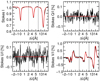 |
Fig. 6 As in Fig. 5 but for the two-component inversion. |
| In the text | |
|
Fig. 7 Response functions integrated over wavelength, added up for all four Stokes parameters and plotted as a function of the logarithm of the optical depth log τ5. Top-left: response to the temperature T. Top-right: response to the line-of-sight velocity vlos. Bottom-left: response to the magnetic field strength B. Bottom-right: response to the inclination of the magnetic field with respect to the observer’s line-of-sight γ. Different colors correspond to different spectral lines. Green: 15 648 Å, red: 15 652 Å, blue: 15 662 Å. The response functions are calculated with the atmosphere resulting from the two-component inversion shown in Fig. 6. |
| In the text | |
|
Fig. 8 Results as a function of the logarithm of the optical depth (logτ5) for the one component inversion: temperature T (top-left), magnetic field strength B (top-right), line-of-sight velocity vlos (bottom-left), inclination of the magnetic field with respect to the observer’s line-of-sight γ (bottom-right). Individual black curves correspond to the inversion of individual pixels. The red curve on the top-left panels shows the temperature stratification from the HSRA model. Red/blue curves on the lower panels indicate vlos = 0 (bottom-left)and γ = 90° (i.e., horizontal magnetic field; bottom-right). |
| In the text | |
|
Fig. 9 Azimuth of the magnetic field in the plane perpendicular to the observer’s line of sight ϕ as a functionof the logarithm of the optical depth logτ5 for the one-component inversion. Individual black curves correspond to the inversion of individual pixels. The average gradient is 700° per optical depth scale decade, indicating multiple rotations of the magnetic field vector within the photosphere. |
| In the text | |
|
Fig. 10 As in Fig. 8 but for the two-component inversion. Red and blue colors represent the first and second components, respectively. Each curve corresponds to a single pixel. |
| In the text | |
|
Fig. 11 Comparison of synthetic Stokes V (upper panel) and I (lower panel) profiles of Fe I 15 648 Å in a two-component atmosphere. The black curve is the inversion result presented in Fig. 6. The red (blue) profile is caused by only the first (second) component, respectively. The respective magnetic field strengths are B = 1147 G and B = 9 G and the filling factor of the component with the strong magnetic field is α = 0.27. We note that both components produce circular polarization signals of similar amplitudes in spite of the very different magnetic fields. The final continuum intensity (lower panel) is about 1.0 (normalized to the quiet Sun value) in spite of the first component featuring very high temperatures (see red lines in the upper-left panel of Fig. 10). |
| In the text | |
|
Fig. A.1 First example of observed (black), fitted with the one-component inversion (red; Sects. 5.1, 6.1), and with the two-component inversion (blue; Sects. 5.2, 6.2), Stokes profiles in a pixel of the red contour in Fig. 4. |
| In the text | |
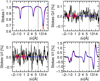 |
Fig. A.2 As in Fig. A.1 but for a second pixel of the red region in Fig. 4. |
| In the text | |
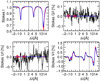 |
Fig. A.3 As in Fig. A.1 but for a third pixel of the red region in Fig. 4. |
| In the text | |
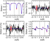 |
Fig. A.4 As in Fig. A.1 but for a fourth pixel of the red region in Fig. 4. |
| In the text | |
Current usage metrics show cumulative count of Article Views (full-text article views including HTML views, PDF and ePub downloads, according to the available data) and Abstracts Views on Vision4Press platform.
Data correspond to usage on the plateform after 2015. The current usage metrics is available 48-96 hours after online publication and is updated daily on week days.
Initial download of the metrics may take a while.