| Issue |
A&A
Volume 616, August 2018
|
|
|---|---|---|
| Article Number | A160 | |
| Number of page(s) | 19 | |
| Section | Stellar structure and evolution | |
| DOI | https://doi.org/10.1051/0004-6361/201732191 | |
| Published online | 31 August 2018 | |
Transition from axi- to nonaxisymmetric dynamo modes in spherical convection models of solar-like stars
1
Max Planck Institute for Solar System Research,
Justus-von-Liebig-Weg 3,
37077
Göttingen,
Germany
e-mail: This email address is being protected from spambots. You need JavaScript enabled to view it.
2
ReSoLVE Centre of Excellence, Department of Computer Science, Aalto University,
PO Box 15400,
00076
Aalto,
Finland
3
Leibniz Institute for Astrophysics Potsdam,
An der Sternwarte 16,
14482
Potsdam,
Germany
4
NORDITA, KTH Royal Institute of Technology and Stockholm University,
Roslagstullsbacken 23,
10691
Stockholm,
Sweden
5
Department of Physics, University of Helsinki,
Gustaf Hällströmin katu 2a, PO Box 64,
00014
Helsinki,
Finland
6
Department of Astronomy, AlbaNova University Center, Stockholm University,
10691
Stockholm,
Sweden
7
JILA and Department of Astrophysical and Planetary Sciences, University of Colorado
Box 440,
Boulder,
CO 80303,
USA
8
Laboratory for Atmospheric and Space Physics,
3665 Discovery Drive,
Boulder,
CO 80303,
USA
Received:
27
October
2017
Accepted:
23
April
2018
Abstract
Context. Both dynamo theory and observations of stellar large-scale magnetic fields suggest a change from nearly axisymmetric configurations at solar rotation rates to nonaxisymmetric configurations for rapid rotation.
Aims. We seek to understand this transition using numerical simulations.
Methods. We use three-dimensional simulations of turbulent magnetohydrodynamic convection in spherical shell wedges and considered rotation rates between 1 and 31 times the solar value.
Results. We find a transition from axi- to nonaxisymmetric solutions at around 1.8 times the solar rotation rate. This transition coincides with a change in the rotation profile from antisolar- to solar-like differential rotation with a faster equator and slow poles. In the solar-like rotation regime, the field configuration consists of an axisymmetric oscillatory field accompanied by an m = 1 azimuthal mode (two active longitudes), which also shows temporal variability. At slow (rapid) rotation, the axisymmetric (nonaxisymmetric) mode dominates. The axisymmetric mode produces latitudinal dynamo waves with polarity reversals, while the nonaxisymmetric mode often exhibits a slow drift in the rotating reference frame and the strength of the active longitudes changes cyclically over time between the different hemispheres. In the majority of cases we find retrograde waves, while prograde waves are more often found from observations. Most of the obtained dynamo solutions exhibit cyclic variability either caused by latitudinal or azimuthal dynamo waves. In an activity-period diagram, the cycle lengths normalized by the rotation period form two different populations as a function of rotation rate or magnetic activity level. The slowly rotating axisymmetric population lies close to what in observations is called the inactive branch, where the stars are believed to have solar-like differential rotation, while the rapidly rotating models are close to the superactive branch with a declining cycle to rotation frequency ratio and an increasing rotation rate.
Conclusions. We can successfully reproduce the transition from axi- to nonaxisymmetric dynamo solutions for high rotation rates, but high-resolution simulations are required to limit the effect of rotational quenching of convection at rotation rates above 20 times the solar value.
Key words: convection / Sun: activity / magnetohydrodynamics (MHD) / dynamo / turbulence / Sun: rotation
© ESO 2018
1 Introduction
Large-scale magnetic fields in late-type stars are thought to be maintained by a dynamo process within or just below the convection zone (e.g., Ossendrijver 2003; Charbonneau 2013). In the relatively slowly rotating and magnetically inactive Sun, the dynamo process is often described by a classical αΩ dynamo, where shearing due to differential rotation produces a toroidal magnetic field from a poloidal magnetic field (Ω effect), and cyclonic convection (α effect) is responsible for regenerating the poloidal field (Parker 1955). Younger late-type stars rotate much faster than the Sun and they also exhibit more vigorous magnetic activity. Theoretical models have long indicated that the differential rotation stays roughly constant as a function of rotation (e.g., Kitchatinov & Rüdiger 1999). The interpretation of observational data is much more challenging. Recent studies show either a mild decrease (e.g., Lehtinen et al. 2016) or a mild increase (Reinhold et al. 2013; Reinhold & Gizon 2015; Distefano et al. 2017) of the relative latitudinal differential rotation, indicating a broad agreement with the theoretical expectation. Therefore, the main effect of increased rotation is a relative dominance of the α effect compared with differential rotation in maintaining the toroidal field. Hence, in view of dynamo theory (e.g., Krause & Rädler 1980), dynamos in rapidly rotating stars operate in a regime in which dynamo action is nearly fully maintained by cyclonic convection (α2 dynamo). Since the early theoretical work it has been known that in the rapid rotation regime the α effect becomes increasingly anisotropic (Rüdiger 1978). An indication of this has been seen at moderate rotation rates (Warnecke et al. 2018). Such an anisotropic α effect can promote nonaxisymmetric large-scale magnetic field configurations (e.g., Rädler et al. 1990; Moss & Brandenburg 1995; Moss et al. 1995; Pipin 2017).
Solar and stellar dynamos tend to manifest themselves very differently in observations. The solar magnetic field exhibits cyclic behavior, in which theactivity indicators vary over an approximate 11 yr cycle; during each activity cycle the polarity of the field reverses, resulting in a magnetic cycle of roughly 22 yr. During one activity cycle, the location in which sunspots appear migrates from mid-latitudes toward the equator. This is commonly thought to trace the latitudinal dynamo wave, that is, a predominantly toroidal component of the large-scale magnetic field that migrates toward the equator. In the Sun, the longitudinal distribution of sunspots indicates that the solar large-scale magnetic field is mostly axisymmetric (e.g., Pelt et al. 2006). In late-type stars with rapid rotation, by contrast, much larger spots located at high latitudes or even polar regions have been observed using Doppler imaging (DI), Zeeman Doppler imaging (ZDI), and interferometry (e.g., Järvinen et al. 2008; Hackman et al. 2016; Roettenbacher et al. 2016). Many studies have reported on highly nonaxisymmetric spot configurations (e.g., Jetsu 1996; Berdyugina & Tuominen 1998), referred to as active longitudes, while especially the indirect imaging of the surface magnetic field using ZDI tends to yield more axisymmetric configurations (Rosén et al. 2016; See et al. 2016).
Especially interesting are the recent results by Lehtinen et al. (2016) regarding a sample of solar-like stars obtained by analyzing photometric light curves. They show a rather sharp transition from stars with magnetic cycles and no active longitudes to stars with both cycles and active longitudes, as the activity level or rotation rate of the stars increases. This result can be interpreted in terms of rapid rotators hosting nonaxisymmetric dynamos and moderate rotators axisymmetric ones. Furthermore, some studies have reported cyclic behavior related to the active longitudes in the form of the activity periodically switching from one longitude to the other on the same hemisphere (Berdyugina et al. 2002) in an abrupt flip-flop event (Jetsu et al. 1993). Other studies report irregular polarity changes between the two longitudes; these are not necessarily connected to the overall cyclic variability of the star (Hackman et al. 2013; Olspert et al. 2015).
The stellar cycles remain poorly characterized, however. Nevertheless, it is clear that many late-type stars exhibit time variability that appears cyclic. This is especially well manifested by studies of stellar samples, such as the intensively investigated Mount Wilson chromospheric activity data base (Baliunas et al. 1995; Oláh et al. 2016; Boro Saikia et al. 2018; Olspert et al. 2018). Even if the range of periods that can be studied is severely limited by the nature of the data because it is too short to study long cycles while the rotational and seasonal timescales limit the periods at the short end, it is clear that stellar cycles are common and even multiple superimposed cycles can occur in one and the same object (Oláh et al. 2009; Lehtinen et al. 2016). There are also indications that the stars tend to cluster into distinct activity branches in a diagram in which the ratio of the cycle period over rotation period is plotted against the rotation rate or activity level (Saar & Brandenburg 1999; Lehtinen et al. 2016; Brandenburg et al. 2017), but the existence of these branches continues to raise debate (Reinhold et al. 2017; Distefano et al. 2017; Boro Saikia et al. 2018; Olspert et al. 2018).
The steadily increasing computational resources have enabled large-scale use of self-consistent three-dimensional (3D) convection simulations to study the mechanisms that drive dynamo action in stars. Recent 3D numerical simulations have been successful in reproducing many aspects of the solar dynamo, such as cyclic magnetic activity and equatorward migration (e.g., Ghizaru et al. 2010; Käpylä et al. 2012; Augustson et al. 2015), the existence of multiple dynamo modes (Käpylä et al. 2016; Beaudoin et al. 2016), and irregular behavior (Augustson et al. 2015; Käpylä et al. 2016, 2017). There are also studies that investigate the dependence of the dynamo solutions on rotation rate, but these have so far either been limited to wedges with limited longitudinal extent (Käpylä et al. 2013, 2017; Warnecke et al. 2016; Warnecke 2018) or the range of rotation rates investigated have been restricted to narrow regions in the vicinity of the solar rotation rate (Strugarek et al. 2017) or three times the solar rotation rate (Nelson et al. 2013). The first indications of stellar dynamos changing from axisymmetric to nonaxisymmetric were reported by Käpylä et al. (2013), Cole et al. (2014), and Yadav et al. (2015b), occurring in the regime of moderate rotation. However, the parameter ranges were rather limited in these studies.
Planetary dynamo simulations (e.g., Ishihara & Kida 2000; Schrinner et al. 2012; Gastine et al. 2012), which typically have much lower density stratification than their stellar counterparts, show that a transition from multipolar to dipolar magnetic field configurations exists at sufficiently rapid rotation. Dipolar solutions have also been found in models with high density stratification and low Prandtl number (Jones 2014; Yadav et al. 2015a; Duarte et al. 2018). Simulations of fully convective stars also favored the occurrence of dipolar solutions (Dobler et al. 2006), but with a transition to multipolar solutions at slower rotation (Browning 2008).
Intriguingly, some ZDI studies suggest that both weak multipolar and strong dipolar magnetic field configurations can occur with very similar stellar parameters in rapidly rotating low-mass (spectral type M) stars (e.g., Morin et al. 2010; Stassun et al. 2011). These observations challenge the simple picture that the M-star dynamos are classical α2 type. Namely, in this case the theoretical expectation is that because the Coriolis number is large owing to long convective turnover times, the α effect becomes strongly anisotropic and results in nonaxisymmetric (multipolar) fields (e.g., Rädler et al. 1990; Moss & Brandenburg 1995; Moss et al. 1995; Pipin 2017). Numerical simulations have revealed bistable dynamo solutions in the rapid rotation regime in which both configurations can be found with the same system parameters but different initial conditions (e.g., Schrinner et al. 2012; Gastine et al. 2012). However, the dipolar solution is typically realized only with a strong initial field.
The goal of the present paper is to carry out a systematic survey of convective dynamo simulations in an attempt to understand the change of magnetic field generation from a young rapidly rotating Sun to its present rotation rate. We are specifically studying the transition of the dynamo solutions from axisymmetric to nonaxisymmetric solutions.
2 Model and setup
We used spherical polar coordinates (r, θ, ϕ) to model the magnetohydrodynamics (MHD) in convective envelopes of solar-like stars. The general model and setup are detailed in Käpylä et al. (2013). For most of the runs we used the full azimuthal extent (0 ≤ ϕ ≤ 2π). However, for some runs we considered only a quarter of the full range (0 ≤ ϕ ≤ π∕2), which we call π∕2 wedges for short. We omitted the poles and thus modeled the star between ± 75° latitude (θ0 ≤ θ ≤ π − θ0, with θ0 = 15°) and modeled only the convection zone of the star in radius (0.7R ≤ r ≤ R, where R is the radius of the star).
2.1 Basic equations
We solve the compressible MHD equations
![Mathematical equation: \begin{align}&\frac{\partial \bm A}{\partial t} = {\bm u}\times{\bm B} - \mu_0\eta {\bm J},\\ &\frac{D \ln \rho}{Dt} = -\bm\nabla\cdot\bm{u},\\ &\frac{D\bm{u}}{Dt} = \bm{g} -2\bm{\mathrm{\Omega}}_0\times\bm{u}+\frac{1}{\rho} \left(\bm{J}\times\bm{B}-\bm\nabla p +\bm\nabla \cdot 2\nu\rho\bm{\mathsf{S}}\right),\\ &T\frac{D s}{Dt} = \frac{1}{\rho}\left[-\bm\nabla \cdot \left({\bm F^{\textrm{rad}}}+ {\bm F^{\textrm{SGS}}}\right) + \mu_0 \eta {\bm J}^2\right] +2\nu \bm{\mathsf{S}}^2,\end{align}](/articles/aa/full_html/2018/08/aa32191-17/aa32191-17-eq1.png)
where A is the magnetic vector potential, u is the velocity, D∕Dt = ∂∕∂t + u ⋅∇ is the Lagrangian time derivative, B = ∇×A is the magnetic field,  is the current density, μ0 and ρ are the vacuum permeability and plasma density, respectively, ν and η are the constant kinematic viscosity and magnetic diffusivity, respectively, g = −GMr∕r3 is the gravitational acceleration where G is the gravitational constant and M is the mass of the star, Ω0 = Ω0(cosθ, −sinθ, 0) is the rotation vector, where Ω0 is the rotation rate of the frame of reference, S is the rate-of-strain tensor, s is the specific entropy; the equations above are solved together with an equation of state for the pressure p, assuming an ideal gas p= (γ − 1)ρe, where e = cVT is the internal energy, T is the temperature, and γ = cP∕cV is the ratio of specific heats at constant pressure and volume, respectively. The radiative and subgrid-scale (SGS) heat fluxes are given by Frad = −K∇T and FSGS = −χSGSρT∇s, respectively, where K is the radiative heat conductivityand χSGS is the SGS heat diffusivity.
2.2 Setup characteristics
The initial stratification is isentropic, where the hydrostatic temperature gradient is defined via an adiabatic polytropic index of nad= 1.5. We initialize the magnetic field with a weak white-noise Gaussian seed field. More details about our initial setup can be found in Käpylä et al. (2013).
Most of our runs use a grid covering the full azimuthal extent, but we perform some comparison runs, labelled with superscript “W” for π∕2 wedges withreduced longitudinal extent. In all cases, we assume periodicity in the azimuthal direction for all quantities. For the magnetic field, we apply perfect conductor boundary conditions at the bottom and both latitudinal boundaries, and at the top boundary we use a radial field condition. Stress-free, impenetrable boundaries are used for the velocity on all radial and latitudinal boundaries. The boundary condition of entropy is set by assuming a constant radiative heat flux at the bottom of the computational domain. The thermodynamic quantities have zero first derivatives on both latitudinal boundaries, leading to zero energy fluxes there. At the top boundary, the temperaturefollows a black body condition. The exact equations for these conditions are described in Käpylä et al. (2013, 2017).
Our simulations are defined by the following nondimensional parameters. As input parameters we quote the Taylor number
![Mathematical equation: \begin{equation*} \textrm{Ta}=\left[2\mathrm{\Omega}_0 (0.3R)^2/\nu\right]^2, \end{equation*}](/articles/aa/full_html/2018/08/aa32191-17/aa32191-17-eq3.png) (5)
(5)
the fluid, SGS, and magnetic Prandtl numbers
 (6)
(6)
where χm = K(rm)∕cPρ(rm) and  are evaluated at rm = 0.85R. The Rayleigh number is obtained from the hydrostatic stratification, evolving a one-dimensional (1D) model, and is given by
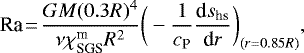 (7)
(7)
where shs is the hydrostatic entropy.
Useful diagnostic parameters are the density contrast
 (8)
(8)
fluid and magnetic Reynolds numbers and the Péclet number,
 (9)
(9)
where kf = 2π∕0.3R ≈ 21∕R is an estimate of the wavenumber of the largest eddies. The Coriolis number is defined as
 (10)
(10)
where  is the rms velocity and the subscripts indicate averaging over r, θ, ϕ, and a time interval during which the run is thermally relaxed and typically covers at least one magnetic diffusion time.
We define mean quantities as averages over the ϕ-coordinate and denote these by an overbar, for example  . The difference between the total and the mean, for example
  , are the fluctuations. Furthermore, we indicate volume averages using
  .
.
For the purpose of this paper, it is convenient to normalize the rotation rate by the solar value, so we define
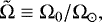 (11)
(11)
where Ω⊙ is the solar rotation rate. Moreover, we use Ω⊙ = 2.7 × 10⁻⁶ s−1, the solar radius R = 7 × 10⁸ m, ρ(0.7R) = 200 kg m−3, and μ0 = 4π × 10−7 H m−1 to normalize our quantities to physical units.
The simulations were performed using the PENCIL CODE1. The code employs a high-order finite difference method for solving the compressible equations of MHD.
3 Results
We consider a number of runs that probe the rotational dependence in the range  = 1–31, corresponding to Co = 1.6–126.5; see Table 1. The range in Co is larger than that in
  because faster rotation leads to lower supercriticality of convection, resulting in a decreased urms and increased Co; see Eq. (10). For some rotation rates we consider different values of the SGS Prandtl number, resulting in different Rayleigh and Péclet numbers and different levels of supercriticality. Runs E, F1, and H are direct continuations of Runs A, B, and C of Cole et al. (2014) and Run F1 was already discussed as Run E4 (Käpylä et al. 2013). Run GW has been analyzed as Run I in Warnecke et al. (2014), as Run A1 in Warnecke et al. (2016), as Run D3 in Käpylä et al. (2016) and in Warnecke et al. (2018). Furthermore, Runs A1 and A2 correspond to 2π extensions of the π∕2 wedges of Set F in Käpylä et al. (2017), whereas Run E corresponds to Set E in Käpylä et al. (2017) and Run B1 in Warnecke et al. (2016). We also include a selection of models (Runs A2, C3, F3) with a lower PrSGS to compare with other studies in which such parameter regimes are explored (e.g., Brown et al. 2010; Nelson et al. 2013; Fan & Fang 2014; Hotta et al. 2016). The numerical studies were carried out over an extended period of time, during which the setups have been continuously refined. This, and the aim to compare to other studies, explains theheterogeneity in the choice of parameters. The physical run time of the saturated stage is denoted by Δ t.
3.1 Overview of convective states
All our models have a density stratification that is much smaller than in the Sun. Therefore, the effects of small-scale convection near the surface and the resulting low local Coriolis numbers in those layers are not captured. This can be achieved only at very high resolution (e.g., Hotta et al. 2014) and is not feasible for parameter studies, such as those carried out in this work. Thus, the effects of rotation are more strongly imprinted in the velocity field near the surfaces of our models than what is expected in actual stars. This is manifested in Fig. 1 where the radial velocity ur is shown for several runs with increasing rotation rate. The size of the convection cells at high latitudes decreases as the rotation rate is increased. Also, we observe the appearance of elongated in latitude columnar structures near the equator at about twice the solar rotation rate. These structures, often referred to as banana cells, persist for all higher rotation rates investigated, their azimuthal and radial extents reducing as a function of rotation, while the latitudinal extent remains roughly constant. The reason for their emergence is the strong rotational influence on the flow and the geometry of the system. Strong rotation tries to force convection into Taylor–Proudman balance resulting in columnar cells that are aligned with the rotation vector. Such cells are connected over the equator only outside the tangent cylinder in a spherical shell, manifesting themselves as elongated structures at low latitudes. Such convective modes can also lead to equatorial acceleration as observed in the simulations and in the Sun (Busse 1970). In the Sun, the small-scale granulation near the surface masks direct observation of larger scale convective modes. However, helioseismic results also suggest that large-scale convective structures exceeding the supergranular scale of 20–30 Mm are weak (e.g., Hanasoge et al. 2012).
To quantify the size of convective structures as a function of rotation we compute the power spectra of the radial velocity near the surface; see Fig. 2. We use a spherical harmonics decomposition to calculate the coefficients  , where ℓ, m are the order of the spherical harmonics and the azimuthal number, respectively. The details on the decomposition can be found in Appendix A. The power at each ℓ is
 (12)
(12)
where Cm = 2 − δm0. We find that for more rapid rotation the radial kinetic energy peaks at smaller scales (higher ℓ, close to ℓ = 100 for Run La) and the kinetic energy at large scales (lower ℓ) becomes smaller; see Fig. 2a. The increasing rotational influence is clearly seen in Fig. 2b, where we plot the value of ℓ at the maximum of the radial velocity spectra as a function of the Coriolis number for all runs. The dependence is consistent with a power law with Co0.26, which is relatively close to the theoretically expected 1/3 scaling for rotating hydrodynamic convection near onset (Chandrasekhar 1961). This is shallower than the slope of about 1/2 found for the horizontal velocity spectra in the simulations of Featherstone & Hindman (2016a). When we only consider the high-resolution runs (blue line in Fig. 2b), we observe a steeper trend (Co0.46). Especially at rapid rotation, the high-resolution runs start deviating significantly from their low-resolution counterparts, and the scale of convection is reduced much more strongly in the former class of runs.
To look at the energy of the radial velocity field at different values of m, we decompose it at the surface, as described in Appendix A. In Fig. 3 we plot the kinetic energy for 0 ≤ ℓ ≤ 10. The total kinetic energy at the surface is decreasing with rotation (panel a), and most of the kinetic energy is contained in the small scales (panel b, orange line). While the fifth nonaxisymmetric mode is mostly constant with increasing rotation (red line), the axisymmetric mode (m = 0) varies strongly and sometimes has comparable or even higher energy than m = 5.
Nonaxisymmetric structures in the velocity field are also visible in Fig. 1 around the equator, in particular for Run La. This is in agreement with previous studies (e.g., Brown et al. 2008), which reported the presence of clear nonaxisymmetric large-scale flows for hydrodynamic simulations in parameter regimes near the onset of convection. These localized nonaxisymmetric structures are similar to the relaxation oscillations, first seen in planetary simulations. Those are explained by realizing that, at intermediate Rayleigh numbers, differential rotation tends to suppress the convective cells and, as a result, they localize in groups across longitude, leaving the rest of the azimuthal domain dominated by the axisymmetric differential rotation.
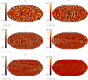 |
Fig. 1 Mollweide projection of radial velocity ur at r = 0.98 R for Runs A2, C3, Ga, H, Ha, and La. |
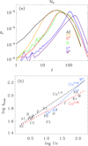 |
Fig. 2 Panel a: normalized power spectra P of the radial velocity as function of degree ℓ for Runs A2, C3, Ga, H, La, and Ma with increasing rotational influence. Panel b: degree of peak power ℓpeak estimated from the power spectra plotted over Coriolis number Co. The runs are indicated with their run names. The red dashed line represents a power law fit including all the runs; the blue dashed line represents the fit for the high-resolution runs, while the black dashed line indicates the expected slope from theoretical estimates (Chandrasekhar 1961). |
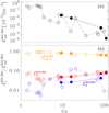 |
Fig. 3 Kinetic energy of the decomposition as a function of Coriolis number Co for all 2π runs showing the total energy (panel a), axisymmetric (m = 0, blue), fifth nonaxisymmetric mode (m = 5, red), and small-scale (l, m > 5, orange) contribution (panel b). All the energies in panel b are normalized to the total energy (panel a). Filled circles connected by a continuous line indicate high-resolution runs. |
3.2 Mean flows
To estimate the rotational influence on the convection we also calculated the volume averaged total kinetic energy density and its contributions; see Table 2. The total kinetic energy density is given by
 (13)
(13)
and the contributions contained in differential rotation and meridional circulation are, respectively,
 (14)
(14)
The contribution from the nonaxisymmetric flows is
 (15)
(15)
The total kinetic energy decreases nearly monotonically as a function of rotation. This clearly shows the rotational quenching of convection, which is related to an increasing critical Rayleigh number in rapidly rotating systems. As a result, the system becomes less supercritical for convection the higher the rotation rate, which is also reflected in the monotonous decrease of the nonaxisymmetric energy that also contains the fluctuations due to convective turbulence. The energy contained in differential rotation and meridional circulation shows a decreasing overall trend as a function of rotation. In general, the capability of the flow to extract energy from thermal energy is decreased by rotation. Comparison to π∕2 wedge simulations indicates some differences in the dynamics of the flow, but it is hard to discern any systematic behavior. For a moderate rotation Run G, the π∕2 wedge (Run GW) has an excess of every type of kinetic energy, while in the rapid rotation regime (Runs I, J, L, M) the flow energies have a tendency to be lower than in the corresponding runs with full azimuthal extent.
3.3 Differential rotation
The rotation also influences the generation of mean flows as for example the differential rotation. To illustrate this, we plot the profiles of angular velocity,  , for six representative runs (Runs A2, C3, Ga, H, Ha, and La) in Fig. 4. We find antisolar differential rotation for the solar rotation rate (Runs A1 and A2), which is consistent with previous numerical studies (e.g., Gastine et al. 2014; Käpylä et al. 2014). This might be due to the overall convective velocities that are too high or the concentration of power that is too high at large spatial scales (Featherstone & Hindman 2016b) in the simulations in comparison to the Sun. The antisolar rotation switches to solar-like at slightly more rapid rotation corresponding to Co = 3.0. For higher rotation rates the differential rotation develops a minimum at mid-latitudes. Such a configuration has been shown to be important in producing equatorward migrating magnetic activity (Warnecke et al. 2014). We also find such minima at moderate rotation, up to roughly seven times solar rotation rate (Run H). At higher rotation rates very little differential rotation is generated overall and the mid-latitude minimum becomes progressively weaker.
We quantify the relative radial and latitudinal differential rotation using
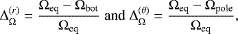 (16)
(16)
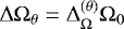
where Ωeq = Ω(R, π∕2) and Ωbot = Ω(0.7R, π∕2) are the angular velocities at the top and bottom of the convection zone at the equator, respectively, and Ωpole = [Ω(R, θ0) + Ω(R, π − θ0)]∕2 is the time averaged angular velocity at the latitudinal boundaries. Negative or positive values of  indicate antisolar (fast poles, slow equator) or solar-like (fast equator, slow poles) differential rotation, respectively. In Table 1 we list these numbers from our simulations and notice that a transition from strong antisolar to significantly weaker solar-like differential rotation occurs at about
  (Co ≈ 3; Run C3). We also plot
  and
and  as functions of Co for all the 2π runs in Fig. 5. There, we indicate the transition point with a vertical dashed line. As we later discuss in detail, this point also marks the change of the dynamo modes from axisymmetric to nonaxisymmetric. From this plot it is evident that, as the rotation increases, both relative differential rotation measures approach zero. From Tables 1 and 2 we also see that near the transition, the rotation profile is sensitive to changes in the convective efficiency, as indicated by the Rayleigh number. In Run C3 with a low
  and lower Rayleigh and Reynolds numbers than in the more turbulent Runs C1 and C2, the rotation profile is solar-like, while in the others it is antisolar. This transition and its sensitivity to the efficiency of convection has been studied in detail by, for example, Gastine et al. (2014) and Käpylä et al. (2014).
We note that  and
and  measure only the difference between certain points and neglect the actual latitudinal variation, which can be more complicated. In the case of wedge geometry the flows near the latitudinal boundaries may not be representative of what takes place at high latitudes in real stars. This can lead to unrepresentative results, in particular for the latitudinal differential rotation in cases where the latitudinal profile is non-monotonic (cf. Karak et al. 2015).
The antisolar regime typically shows strong negative radial and latitudinal shear (Gastine et al. 2014), whereas magnetic fields tend to quench the differential rotation (e.g., Fan & Fang 2014; Karak et al. 2015). Our results are in agreement with those aforementioned studies. Another important aspect is the dependence of absolute differential rotation, defined as
 (17)
(17)
on the rotation rate itself. The broad range of probed rotation rates allows us to search for a power-law behavior of the form
 (18)
(18)
In Fig. 6, we do not find, however, a single power law that would describe the behavior at all rotation rates. For slow and moderate rotation, up to  , we fit a slope of q ≈ −0.08, while for the highest rotation rates investigated,
  , we find a steeper power law with q ≈−0.96.
In Table 3, we compare our results with those of some observational studies (Reinhold & Gizon 2015; Lehtinen et al. 2016) and a mean-field model (Kitchatinov & Rüdiger 1999). Our results for the low to intermediate rotation rates agree with these studies, but the power law we find for the rapid rotation regime is much steeper and therefore in disagreement with them. This disagreement cannot be explained by the lack of supercriticality as the high-resolution runs show even weaker latitudinal differential rotation than their low-resolution counterparts. However, the magnetic fields in the rapidly rotating high-resolution runs (Ha, La, and especially in Ma) are generally stronger than in the lower resolution runs, possibly also contributing to the reduced differential rotation (cf. Käpylä et al. 2017).
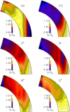 |
Fig. 4 Normalized angular velocity Ω(r, θ) of Runs A2, C3, Ga, H, Ha, and La. The dashed lines denote the radius r = 0.98 R, which is used for the further analysis. |
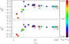 |
Fig. 5 Relative latitudinal differential rotation |


Summary of the runs.
Volume averaged kinetic and magnetic energy densities in units of 105J m−3.
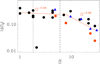 |
Fig. 6 Modulus of the absolute latitudinal differential rotation, |
3.4 Overview of magnetic states
All the runs discussed in this work produce large-scale magnetic fields. Similar runs were recently analyzed by Warnecke et al. (2018) using the test-field method, which measured significant turbulent effects contributing to the magnetic field generation. Therefore, we attribute the magnetic fields seen in the current runs to the turbulent dynamo mechanism. To describe the magnetic solutions, we first look at the volume-averaged magnetic energy densities. We define these densities analogously to their kineticcounterparts. We use
 (19)
(19)
for the totalmagnetic energy density,
 (20)
(20)
for the contribution of mean toroidal and mean poloidal fields, and
 (21)
(21)
for the contribution of fluctuating magnetic fields. These quantities are listed in Table 2. We find that for all the runs, the contributions from fluctuating magnetic fields dominate the magnetic energy. The axisymmetric contributions contain on the order of 5% to 10% of the total magnetic energy in the majority of the runs, and exceeds 15% only in Runs C3, F3, K1, and K2. These runs are characterized either by a low PrSGS (C3 and F3) or rapid rotation (K1 and K2), both leading to reduced supercriticality of convection.
In contrast to the kinetic energy, we do not find a clear trend for magnetic energies as a function of rotation rate. In the rapid rotation regime, the high-resolution runs La and Ma exhibit magnetic fields with an energy that significantly exceeds the kinetic energy by factors of roughly 3 and 8, respectively. If we look at the radial profile of the magnetic energy density for a selection of runs (Fig. 7), we find that the magnetic field in the upper half of the convection zone increases with rotation. As discussed earlier, we observe a simultaneous, nearly monotonic, decrease of the kinetic energy as a function of rotation rate. Therefore, the ratio of the magnetic to kinetic energies, which is a measure of the dynamo efficiency, is actually steeply increasing as a function of rotation, as can be seen from Fig. 8. We find that in the low-resolution cases the dynamo is clearly less efficient in the rapid rotation regime in comparison to the high-resolution cases. We also observe that the π∕2 wedge runs produce a far more efficient dynamo in the rapid rotation regime than the corresponding low-resolution runs with full azimuthal extent. This is possibly explained by the somewhat higher stratification and Rayleigh numbers in the π∕2 wedge runs in comparison to those in the low-resolution full 2π models. We can conclude that the convective efficiency directly influences the dynamo efficiency and therefore, the magnetic energy production.
In Fig. 5 we studied the dependence of the overall magnetic topology on the amount of differential rotation generated inthe system. The ratio of poloidal to toroidal magnetic energies, shown with the color of the symbols, changes systematically from mostly poloidal field configurations at very low rotation rates to toroidal field configurations at moderate and rapid rotation. The energy ratio gradually decreases, and with rotation rates exceeding the antisolar to solar transition point, dominantly toroidal fields are seen. The strongest toroidal fields are generated for moderate rotation. At the highest rotation rates, the ratio of toroidal and poloidal becomes again lower in the high-resolution runs, while the low-resolution counterparts fail to show systematic behavior. In the run with the highest rotation rate, Ma, the poloidal component again dominates. By inspecting Table 2, we notice that the models with reduced ϕ extent tend to produce a larger poloidal to toroidal energy ratio than the corresponding runs covering the full azimuthal extent.
To investigate the spatial structure of the magnetic field, we show in Fig. 9 snapshots of Br for six representative runs. At low rotation rates, most of the magnetic field is concentrated in the downflows between the convective cells, while at high rotation rates, the scale of convection, still clearly affecting the magnetic field, thereby leaving a small-scale imprint on it, is significantly reduced. Nevertheless, global-scale magnetic field configurations clearly emerge in the high-latitude regions. It is immediately apparent that a nonaxisymmetric large-scale pattern is visible in all cases. In the slowly rotating cases, the nonaxisymmetric component is subdominant and the equatorial symmetry of the field is clearly dipolar (antisymmetric with respect to the equator). In all the runs with solar-like differential rotation, however, the field configuration is observed to be symmetric (or quadrupolar) with respect to the equator, even though a more detailed analysis revealed that the parity of the solutions is not pure. A weaker antisymmetric (dipolar) component is present at all times and the global parity undergoes some fluctuations. The quadrupolarcomponent remains most significant at all times, however. This result is in agreement with some ZDI measurements of solar-like stars (e.g., Hackman et al. 2016; Rosén et al. 2016). However, we should point out that our results can be influenced by the wedge assumption in latitude and need to be verified in full spherical geometry.
We also depict the overall nonaxisymmetry of the large-scale magnetic field solutions with the shape of the symbol in Fig. 5. Again, on the lower rotation side of the break point identified, the magnetic fields are mostly axisymmetric (circular symbol). On the rapid rotation side, the fields exhibit a significant nonaxisymmetric component (triangles) and finally turn into completely nonaxisymmetric components (stars). The resolution also plays a significant role in the nonaxisymmetry measure. The higher resolution runs show preferentially nonaxisymmetric configurations, while the lower resolution runs turn back to axisymmetry at the highest rotation rates investigated.
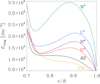 |
Fig. 7 Radial profiles of the total magnetic energy density Emag averaged over time, latitude, and azimuth for Runs A2, C3, Ga, Ha, La, and Ma. |
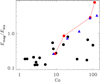 |
Fig. 8 Ratio of total magnetic to kinetic energies Emag∕Ekin as a functionof Coriolis number Co. The red filled symbols (connected by a line) denote high-resolution runs. Blue triangles refer to π∕2 wedge runs. |
3.5 Degree of nonaxisymmetry
Large-scale nonaxisymmetric magnetic fields, as seen in Fig. 9, are included in the definition of  in Table 2, as this quantity is the difference between total and azimuthally averaged (mean) magnetic energies. This term, therefore, contains both small-scale fluctuations and large-scale nonaxisymmetric contributions. Thus, the diagnostics introduced so far only roughly describe the large-scale fields in the system.
To obtain a more complete picture, we perform a spherical harmonics decomposition of the radial components of the vector fields at r = 0.98 R with the method described in Appendix A. The m = 0 mode contains the axisymmetric (mean) part of the radial magnetic field, the m = 1 is the first nonaxisymmetric mode, m = 2 is the second mode, and so on. For the π∕2 wedges, the first nonaxisymmetric mode is m = 4. The energies of the modes resulting from the decomposition are listed in Table 4. Depending on the dominant large-scale component, we call the magnetic fields nonaxisymmetric or axisymmetric even though their small-scale contributions, which are always nonaxisymmetric, might be more energetic.
The distribution of the radial magnetic energy density near the surface of the star is presented in Fig. 10a as a function of Co. We show the axisymmetric and magnetic energy in the large-scale nonaxisymmetric field (1 ≤ ℓ ≤ 5) normalized by the total magnetic energy. We find an inversion between the energies in the axisymmetric and nonaxisymmetric components, which also coincides with the transition from antisolar- to solar-like differential rotation at Co ≈ 3. The runs show a nonaxisymmetric magnetic field until Co ≈ 70, but at higher Co the high-resolution runs remain nonaxisymmetric, while the low-resolution runs return to an axisymmetric configuration, indicating that high resolution is needed at such high rotation rates to capture the small scales. This could explain the lack of nonaxisymmetric solutions in the study of Brown et al. (2010). This conjecture is supported by the fact that in the higher resolution simulations of Nelson et al. (2013) significantly clearer nonaxisymmetric features are seen (their Figs. 4–6), although they are confined to low latitudes. Those simulations were made with  , albeit with a lower thermal Prandtl number and different viscosity and diffusivity profiles than in the current simulations (cf. Appendix A of Käpylä et al. 2017, for a comparison of different setups). Our Runs C3 and F3 also produce strong nonaxisymmetric large-scale fields at high latitudes despite their lower values of PrSGS. This could be an indication of the influence of the latitudinal boundaries in the current simulations.
The simulations of Fan & Fang (2014) and Hotta et al. (2016), on the other hand, used the solar rotation rate and a further decreased thermal Prandtl number resulting in a laminar heat transport to force a solar-like rotation profile. The large-scale magnetic fields in those simulations are characterized by dominant low-latitude axisymmetric fields, which show apparently random polarity reversals. The results of these studies are most closely related to our slowly rotating Runs A1, A2, and B, which also produce predominantly axisymmetric large-scale fields, although with antisolar differential rotation. This seems to suggest that axisymmetric fields are preferred at slow rotation irrespective of the differential rotation profile.
From Table 4 we notice that m = 1 is the first large-scale nonaxisymmetric mode excited as the rotation increases. Some higher m modes get excited, too, but they remain, on average, subdominant compared to the m = 1 mode. Therefore, the runs are well described by the m = 0 and m = 1 modes, shown in Fig. 10b. The axisymmetric energy is dominant at slow rotation, Co ≤ 3, while in the range 3 ≤Co ≤ 72 the first nonaxisymmetric mode is dominant, but its strength decreases for the low-resolution runs for Co > 20, and eventually there is a return to an axisymmetric configuration at the highest values of Co. For the high-resolution runs, however, the m = 1 mode energy keeps increasing until the highest rotation rates investigated.
Energy densities of the radial magnetic field and dynamo cycle properties.
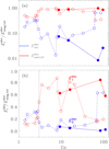 |
Fig. 10 Axisymmetric mean (m = 0, blue) energy vs. nonaxisymmetric large-scale (m = 1, 5; red) energy fraction at the surface (panel a). Axisymmetric mean (m = 0; blue) energy fraction vs. the first nonaxisymmetric mode (m = 1; red) energy fraction (panel b). The dotted black line denotes the axisymmetric to nonaxisymmetric transition at region Co ≈ 3. In both plots, the dashed red and blue lines connect 2π runs; filled symbols, connected with solid lines, denote the high-resolution runs. |
3.6 Magnetic cycles
The time evolution of the magnetic field is not cyclic in the sense that there are not necessarily polarity reversals in all the runs. Yet, we see cyclic variations around the mean magnetic energy level, albeit with a poorly defined cycle length. This would match with an observer’s viewpoint, as most often only light curve variability is observable while the surface magnetic evolution is hidden. Therefore, it makes sense to try to determine the timescale of this variability for all the runs – not only those for which we can identify cyclic polarity reversals from the butterfly diagram (the runs underlined in Table 4). By counting how many times the mean magnetic energy level is crossed, sometimes referred to as the syntactic method (Chen 1988, Chap. 9.4), we can assign a characteristic time scale of change, τcyc. For some of the runs, the time-latitude variability would provide another, more straightforward, way to determine the cycle length. For consistency, this approach is used to determine the cycle periods for all the runs. A comparison with cycle determination using all magnetic field components at all latitudes shows good agreement between these two methods for these kinds of simulations (Warnecke 2018). The last column in Table 4 shows τcyc. We use the syntactic method on the dominant modes (m = 0 and m = 1) and indicate those by a subscript. The syntactic method, however, has a limitation in that counting the fluctuations around a mean value means that we always count at least one oscillation. This makes the τcyc values for Runs D, K2, and Ma questionable, as they are roughly half of the run time of the simulations. This time is denoted by Δ t and is listed in Table 1. One could instead determine the characteristic time by running the aforementioned runs for a longer time. Retrieving cycle periods of the same order as the data set lengths, however, is not uncommon in observational studies (see e.g., Baliunas et al. 1995), so we have decided to retain these values with the other, more trustworthy values, in our analysis.
In the Runs A1, A2, and B, all with antisolar differential rotation profiles, we do not see much time dependence in the time–latitude (butterfly) diagrams of the mean toroidal magnetic fields; see the upper left panel of Fig. 11 for an example from Run A2. Starting from Runs C1, C2, and C3 onward to higher rotation rates (other panels of Fig. 11), however, more systematic patterns are discerned in the time series and butterfly diagrams. Runs C1 and C2 present two interesting cases, as it is very rare to obtain cyclic dynamo solutions in the regime of antisolar rotation profiles (e.g., Karak et al. 2015; Warnecke 2018), which these runs clearly possess. Furthermore, it is clear that simulations with a 2π azimuthal extent are capable of producing oscillating dynamo solutions at lower rotation rates than the corresponding π∕2 wedges (see comparison in Warnecke 2018). In the rapid rotation regime, the time variability is always linked to the nonaxisymmetric component, especially in the high-resolution runs.
After estimating the characteristic time, we can determine the activity cycle period as Pcyc = τcyc, see how it varies with rotation, and compare these values with observational results (Saar & Brandenburg 1999; Lehtinen et al. 2016). We show the results in Fig. 12a, in which we plot the ratio of rotation to activity period against the Coriolis number. We see that the transition line Co = 3 divides the runs into two populations: one in which the antisolar axisymmetric runs cluster and another in which the solar-like nonaxisymmetric runs cluster. The former population is located in the upper left corner of the plot showing a negative slope. At this location, Noyes et al. (1984) found, however, a population of stars with a positive slope. Brandenburg et al. (1998) denoted this the inactive (I) branch – to distinguish it from another active (A) one. At even higher rotation rate, Saar & Brandenburg (1999) found yet another superactive (S) branch. This branch has a negative slope, which coincides with our solar-like nonaxisymmetric population (shown in red in Fig. 12a). The rapidly rotating runs yield Co−0.50, which agrees with the slope Co−0.43 determined by Saar & Brandenburg (1999) for the S branch. However, we cannot clearly identify an A branch nor a transition between the A and S branches, which are clearly present in Saar & Brandenburg (1999). The dashed vertical line denotes the observational transition of stars without active longitudes to those with active longitudes in a sample of solar-like rapid rotators (Lehtinen et al. 2016). We note that in our simulations, active longitudes occur for considerably lower Coriolis numbers (Co > 3, corresponding to the leftmost dotted line).
The best available measure of the magnetic activity from our simulations is the ratio of magnetic to kinetic energy, which can be directly thought of as a measure of the efficiency of the dynamo; see Fig. 8. Figure 12b shows the rotation–activity period ratio as a function of this quantity. In this plot, our runs again cluster near the I branch and a well separated A–S branch. In contrast to Fig. 12a, the correlation on the I branch now appears positive, but there are not enough points to reliably conclude whether either of the correlations seen on this branch are significant. The S branch still remains inseparable, but the population of runs falling onto this branch shows a distinct negative slope.
In Fig. 12c we show a comparison between observational results and the models of Strugarek et al. (2017) using again the Coriolis number on the x axis. In this representation, although the I branch still clearly exists, none of the modeled points coincide with the observed I branch. Instead, the slowly rotating models cluster at lower Coriolis numbers than the observed stars on the inactive branch, although their cycle ratios would rather well match with those of the observed population. The Sun is not reproduced in any of those runs.
The moderate and rapid rotation runs are consistent with the S branch behavior. Strugarek et al. (2017) and the π∕2 wedges of this study have a slope most closely matching the observed points of Lehtinen et al. (2016). The runs covering the full longitudinal extent have significantly shallower slope than the data points for the observed stars. The fact that the Strugarek et al. (2017) results coincide so well with those from our π∕2 wedges, where the large-scale nonaxisymmetric modes are absent, suggests that also the former models tend to become axisymmetric. It needs to be seen to what extent this can be explained by those runs not being sufficiently supercritical; see again Appendix A of Käpylä et al. (2017) for a comparison of different setups. This is clearly seen in our low-resolution models, in which the magnetic field becomes axisymmetric at rapid rotation, while in their high-resolution counterparts the magnetic field remains nonaxisymmetric. We note that our first run with solar-like differential rotation, C3, is also the first showing nonaxisymmetric magnetic field. This is in disagreement with observations, as the Sun has a mostly axisymmetric field. Therefore, we conclude that the model of Strugarek et al. (2017) with lower convective velocities, and thereby less supercritical convection, can better reproduce the behavior in the proximity ofthe solar rotation rate. At rapid rotation regime, however, their convective velocities are too low for the models to capture the transition at all, while ours are too large and push it to Coriolis numbers that are too low.
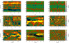 |
Fig. 11 Mean toroidal magnetic field |

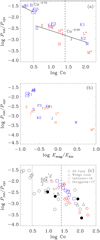 |
Fig. 12 Ratio of the rotation period to the cycle period as a function of Coriolis number (panel a). The two black lines indicate the fit to the axisymmetric and rapid rotation runs, respectively. The vertical lines denote the nonaxisymmetric transition found in our simulations (dotted; Co ≥ 3) and from the observational study of Lehtinen et al. (2016) (dashed), respectively. Runs are plotted after their labels. The color indicates the mode chosen for calculating τcyc: blue for m =0, red for m = 1. Prot ∕Pcyc as function of activity, represented by Emag∕Ekin is shown in panel b. Panel c: comparison between the results presented in this paper, Lehtinen et al. (2016), and Strugarek et al. (2017). Black circles and triangles denote high resolution and π∕2 wedges in our set, respectively. The gray dots indicate M dwarfs and F and G stars from Brandenburg et al. (2017). |
3.7 Azimuthal dynamo waves
In stars that rotate more rapidly than the Sun, spots tend to emerge at high latitudes and are unevenly distributed in longitude. These preferred locations for starspot appearance are called active longitudes (Jetsu 1996; Berdyugina & Tuominen 1998). A phenomenon that has recently been related to active longitudes from models (Cole et al. 2014) and also observations (see e.g., Lindborg et al. 2013) is what is now called azimuthal dynamo wave (ADW). This term refers to active longitude systems that migrate in the orbital reference frame of the star. A useful comparison is the latitudinal dynamo wave visible in the Sun. This dynamo wave shows a dependence in latitude, which is visible as the appearance of sunspots at lower latitudes as the solar cycle progresses, but the spots do not appear with a preferential location in longitude. Instead of its latitude depending on time, in the ADW the longitude of the nonaxisymmetric spot-generating mechanism changes periodically in time, thereby migrating in the rotational frame of reference. Such migration was already predicted from early linear dynamo models (e.g., Krause & Rädler 1980) and the special case of nonmigratory nonaxisymmetric structure could also be interpreted as a standing ADW. The crucial difference between latitudinal and ADWs is that the polarity reversal is always associated with the former, while not necessarily with the latter. The migration direction has been observed to be preferentially prograde (see e.g., Berdyugina & Tuominen 1998; Lindborg et al. 2013; Lehtinen et al. 2016), but also a standing wave for σ Gem and a retrograde wave for EI Eri have been reported (Berdyugina & Tuominen 1998).
We inspect all our runs with a significant m = 1 mode for the existence of ADW. The results for the reconstruction of the first nonaxisymmetric mode of the radial magnetic field as functions of time and longitude for Runs C3, Ga, Ha, and La are shown in Fig. 13 for 60° northern latitude. In all the runs presented here, the m = 1 mode is rigidly rotating and has a different pattern speed than the gas. To verify that the magnetic field is detached from the flow, we overplot the expected advection due to differential rotation with black–white lines at the same latitude. If the magnetic field was advected by the mean flow, its maxima and minima would fall on this line. In the range 3 ≤ Co ≤ 68, the magnetic field follows a pattern that is different from the differential rotation at the surface of the star at all latitudes.
The parameters related to the ADW are listed in columns 11–14 of Table 4. The period of the ADW, PADW, is calculated using the first derivative with respect to time of the maximum of the phase of the m = 1 mode, averaged over time and latitude. We compare it with the bulk rotation, PADW∕P0, and the differential rotation, PADW∕PDR, where P0 = 2π∕Ω0 and }\rangle_{\theta}$](/articles/aa/full_html/2018/08/aa32191-17/aa32191-17-eq40.png) , respectively, and indicate the direction of the wave, retrograde (R, westward) or prograde (P, eastward), in the column marked D. A retrograde wave is moving in the opposite direction with respect to the bulk rotation. Therefore, its period is longer than the rotation period. On the other hand, a wave moving in the prograde direction has a shorter period. In most of our cases, we find retrograde ADWs, but there are some cases (Runs J, K1, La, Ma) in which the behavior is different. Runs J and K1 are characterized by rapid rotation and a low value of magnetic energy and the ADW has a smaller amplitude than in the other cases. In Runs Ma, La, and J the dynamo wave is drifting very slowly2. During the saturated stage, these represent standing waves rather than migratory phenomena (therefore the identifier SW in Table 4). Their almost insignificant migrations occur in opposite directions with Runs J and Ma showing prograde migration and Run La exhibiting retrograde migration. In the parameter range included in this study, the retrograde migration is clearly the dominant regime. The magnetic cycle does not seem to be related in any way to the migration period of the ADW.
, respectively, and indicate the direction of the wave, retrograde (R, westward) or prograde (P, eastward), in the column marked D. A retrograde wave is moving in the opposite direction with respect to the bulk rotation. Therefore, its period is longer than the rotation period. On the other hand, a wave moving in the prograde direction has a shorter period. In most of our cases, we find retrograde ADWs, but there are some cases (Runs J, K1, La, Ma) in which the behavior is different. Runs J and K1 are characterized by rapid rotation and a low value of magnetic energy and the ADW has a smaller amplitude than in the other cases. In Runs Ma, La, and J the dynamo wave is drifting very slowly2. During the saturated stage, these represent standing waves rather than migratory phenomena (therefore the identifier SW in Table 4). Their almost insignificant migrations occur in opposite directions with Runs J and Ma showing prograde migration and Run La exhibiting retrograde migration. In the parameter range included in this study, the retrograde migration is clearly the dominant regime. The magnetic cycle does not seem to be related in any way to the migration period of the ADW.
3.8 Timevariation and flip-flop phenomenon
In some cases we find an equatorward migrating oscillatory magnetic field in the initial stages of the simulation (e.g., Runs G and H), see Fig. 11. Later, however, the dominant dynamo mode changes to a nonaxisymmetric mode soon after the large-scale field reaches dynamically significant strengths. This behavior has been found in Käpylä et al. (2013), where the π∕2 and 2π versions of Run F1 have been compared. Thus, we conclude that a reduced ϕ extent significantly changes the behavior of the dynamo by suppressing the large-scale nonaxisymmetric modes (m = 1, 2, 3). Also, we observe that for cyclic solutions to emerge in π∕2 wedges, we require a generally higher Coriolis number than in runs with full azimuthal extents.
Time variations are also seen in the cases of nearly purely nonaxisymmetric solutions; one such example is the high-resolution Run La. The magnetic field in this run forms two active longitudes that remain fixed on the stellar surface, having opposite polarities in each hemisphere, but exhibiting a quadrupolar symmetry with respect to the equator. The weak axisymmetric component also exhibits time variability, as can be seen from the butterfly diagram plotted in Fig. 11. Both the axi- and nonaxisymmetric components develop time variability over a similar timescale of roughly three years. The strength of the active longitudes is modulated on this timescale in such a way that those in the same hemisphere grow simultaneously (see Figs. 13 and 14) while those on the opposite hemisphere decay, followed by a reversed behavior (see Fig. 14). However, there are no clear polarity reversals that could be related to this time variation. In other words, we observe that maximum and minimum on the same hemisphere never switch in intensity, as happens in the flip-flop phenomenon (Berdyugina & Tuominen 1998; Hackman et al. 2013). It has been postulated that a polarity reversal of the active longitudes would happen during a flip-flop event and would be observable through ZDI (e.g., Carroll et al. 2009; Kochukhov et al. 2013), but the effect of ADWs has never been considered, making these conclusions uncertain.
To see whether flip-flops can occur in systems in which there is a competition between the m = 0 and m = 1 modes, we now analyze Run Ga in detail. As discussed in Sect. 3.7, this run exhibits an ADW that is migrating in the retrograde direction. To better see the time evolution of the active longitudes, this migration has to be removed, as carried out in Fig. 15, lower panel. After this systematic motion is removed, however, as in the case of La, the active longitudes are not switching in intensity between maxima and minima, but grow and decay together on the same hemisphere, while out of phase in the opposite hemisphere. In Run J, producing only a very weak dynamo solution with almost a standing ADW, a polarity change can, however, be detected, as is depicted in Fig. 15, upper panel. The active longitudes are seen to stay nearly fixed in the orbital frame of reference, and after quasi-regular time points, the polarity of both reverses quite abruptly. In this case the magnetic field is clearly subdominant with respect to the velocity field, but nevertheless the advection by the differential rotation explains the time evolution of the active longitudes very poorly. Distinguishing between such a polarity reversal and the mere migration of the active longitude poses a challenge to the observations. According to our models, the migration speeds are always very distinct from the rotation periods, so any behavior caused by such systematic movement would appear smooth to a real flip-flop.
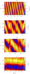 |
Fig. 13 Reconstruction of the m = 1 mode of the magnetic field at the surface of the star for Runs C3, Ga, Ha, and La at θ = +60°. The black and white line indicates the path due to differential rotation alone. |
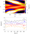 |
Fig. 14 Standing dynamo wave of Run La. Lower panel: time variation of the four regions indicated in the upper panel. |
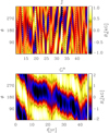 |
Fig. 15 Upper panel: flip-flop for Run J. The dashed line is the differential rotation at θ = +45°. Lower panel:same as Fig. 13, but at θ = +45°, for Run Ga. The ADW has been de-migrated to better show the active longitudes. |
4 Conclusions
In this paper, we have performed an extensive study of the effect of rotation rate on convection-driven spherical dynamos, covering a range from 1 to 31 times the solar value, Ω⊙, corresponding to Co = 1.6 to 127. The dependence of stellar dynamos on rotation speed has been assessed over a range that is much wider than what has been studied previously. For example, Strugarek et al. (2017) studied the change of cycle frequency while changing the rotation rate by a factor of two, resulting in a change in Co of about a factor of three. We found that, for Ω ≳ 1.8Ω⊙ (Co ≳ 3), nonaxisymmetric modes are excited and ADWs are present; see Table 5. The most commonly excited configuration in our models is the m = 1 mode accompanied with an m = 0 mode comparable (for moderate rotation) or subdominant (for rapid rotation) in strength. The magnetic field near the surface is symmetric (quadrupolar) with respect to the equator in all cases with an antisolar differential rotation profile. The axisymmetric part of the magnetic field is more toroidal at moderate rotation, while preferentially more poloidal configurations are indicated from the highest rotation rates studied. In the slow rotation regime with antisolar differential rotation, the solutions are preferentially axisymmetric and poloidal.
The same pattern over the azimuthal direction can be seen observationally in the distribution of active longitudes or the magnetic field geometries of stars with different rotation rates. Lehtinen et al. (2016) found from time series photometry of active solar-type stars that there is an onset of active longitudes at around Co ≈ 25, corresponding to  . Similarly, surface magnetic field mapping using ZDI has shown that solar-type stars have a transition between axisymmetric poloidal and nonaxisymmetric toroidal field geometries at around Co ≈ 13 (or Ro = Prot∕τc ≈ 1; Donati & Landstreet 2009; See et al. 2016), where τc is the convective turnover time. This split is not absolute and the rapidly rotating stars can still alternate between toroidal and poloidalfields (Kochukhov et al. 2013). Moreover, Rosén et al. (2016) observed that for rapid rotators the degree of nonaxisymmetry tends to increase toward more poloidal field geometries. This may indicate a similar behavior as in the high-resolution models, which develop nonaxisymmetric poloidal fields at the highest rotation rates. We note here that we calculate the toroidal and poloidalfields from the axisymmetric mean field in the whole convection zone, while in observations the total surface field is used.
The differences in the rotation rates and Coriolis numbers of the axisymmetric to nonaxisymmetric transition between observations and simulations may be due to several factors. First, the criteria for detecting nonaxisymmetric structures may not be fully comparable between the various studies. Second, the observational studies use semiempirical values of the convective turnover time τc while in this study we used the definition τc = 2πurms∕0.3 R. Lastly, it is worth noting that the simulations do not occupy the same parameter space as real stars. Furthermore, a different value of Co could just be explained by a different depth in the star where the dynamo is mainly driven, as urms has a strong radial dependency. The observations do not show any indication that the most rapidly rotating stars would again have axisymmetric fields, as is the case with the low-resolution runs in this study. The difference in behavior between high- and low-resolution runs, for which low-resolution runs turn back to axisymmetric fields and high-resolution runs remain nonaxisymmetric may simply be a symptom of the inability of the low-resolution runs to capture sufficiently small scales.
In our set of runs, we found mostly retrograde ADWs in contrast with observations of solar-like stars that show a preference for prograde direction (Lehtinen et al. 2016). The prograde pattern speeds may be analogous to those seen in the Sun. Its supergranulation pattern is found to rotate a few percent faster than the gas at the surface (Gizon et al. 2003). Similarly, magnetic tracers including sunspots are seen to rotate faster than the gas (Pulkkinen & Tuominen 1998). The occurrence of prograde pattern speeds is theoretically associated with the near-surface shear layer of the Sun (Green & Kosovichev 2006; Busse 2007; Brandenburg 2007). Thus, a reason for this discrepancy could be the fact that we simulate only the stellar convection zone and do not include the near-surface shear layer, which should lead to a prograde directed wave.
In the interval 1–1.8 Ω⊙, corresponding to Co = 1.6–2.8, we find antisolar differential rotation, which is in agreement with previous studies such as Käpylä et al. (2014) and Gastine et al. (2014). We do not see any oscillatory behavior of the magnetic field in the interval Co = 1.6–2.4, whereas close to the transition from antisolar to solar rotation profiles, at Co = 2.6–2.8, even systems with antisolar rotation profiles produce clear cycles in their axisymmetric fields. This seems to be quite a robust finding, as this behavior persists even when the efficiency of convection is varied. Cyclic magnetic activity has been seen in giants and subgiants that are believed to have antisolar differential rotation profiles (Weber et al. 2005; Kővári et al. 2007; Harutyunyan et al. 2016), which, according to our results, would be possible in a narrow region near the break point from antisolar (and axisymmetric) to solar (and nonaxisymmetric) behavior (see Table 5). In dwarfs, antisolar differential rotation is indicated only indirectly through the occurrence of enhanced activity at slow rotation for  (Brandenburg & Giampapa 2018).
In the rapid rotation regime, both dominantly axisymmetric and nonaxisymmetric solutions produce time variability of very different nature, which, however, occurs over similar timescales and produces similar magnitudes of variations, at least in terms of the surface magnetic field strength. In the axisymmetric case, these relate to the latitudinal dynamo wave and are accompanied by a polarity change. In the majority of the nonaxisymmetric cases, the time variability relates to the changing activity levels of active longitudes on different hemispheres with no associated polarity change. In one low-resolution case that produces only a very weak dynamo, we found a solution that also shows flip-flop type polarity reversals, but this particular parameter regime needs to be studied with high-resolution runs. The drift period of the active longitude system in the orbital frame of reference identified in almost every simulation seem to be decoupled from the magnetic activity cycle, but together with the variations in the active longitude strengths can be thought to give rise to an ADW. Also observationally the occurrence of cycles is not related to the axisymmetry of the stellar magnetic fields. Activity cycles are observed on slow and fast rotating stars alike, regardless of whether they have active longitudes or not (Lehtinen et al. 2016).
Our extensive study of the dependence on rotation rates allowed us to investigate the existence of activity branches (see e.g., Saar & Brandenburg 1999; Distefano et al. 2017; Reinhold et al. 2017). In our Prot∕Pcyc versus Co plot, the runs areseparated into two populations: one for the axisymmetric runs at low Coriolis numbers, whose slope of Co−0.73 seems to be similar to that found in the π∕2 wedges of Warnecke (2018), the other at higher Co representing the nonaxisymmetric population, whose slope of Co−0.50 is close to the superactive branch reported in Saar & Brandenburg (1999) and whose behavior resembles that of the transitional branch of Distefano et al. (2017). However, when comparing to observations, our inactive population does not match the inactive branch seen in observational studies (e.g., Noyes et al. 1984; Brandenburg et al. 1998, 2017). A possible explanation for this discrepancy could reside in the different ways of calculating τc in observationsand simulations. Also, we do not find any clear separation between active and superactive branches. Moreover, we studied the behavior of Prot∕Pcyc as a function of magnetic activity (represented, in our case, by the ratio Emag∕Ekin). In this case, the axisymmetric population seems to have a positive slope, as seen in observations. Anyway, our sparse sample at low rotation and the inability to reliably compute the chromospheric activity index  from the models do not allow us to draw any significant conclusion. We also compare our results with the numerical study of Strugarek et al. (2017). In contrast with our simulations, their solutions show only axisymmetric behavior. This, and the fact that in the rotation-activity plot their results lay close to our models with reduced ϕ extent, make us believe that the resolution used in this study was not enough to allow for nonaxisymmetric solutions. We considerthis as a further proof of the importance of using high resolution when investigating high rotation regimes.
Our results confirm that the scale at which the power spectrum of the velocity field peaks shifts to higher values of ℓ with increasing rotation speed, indicating the presence of smaller convective cells at rapid rotation (Chandrasekhar 1961). Our results have also demonstrated that sufficiently high numerical resolution is important for allowing the m = 1 nonaxisymmetric structure to develop. The wedge assumption in the azimuthal direction was not found to be a a good assumption for rapidly rotating stars. First, this assumption suppresses the nonaxisymmetric modes that emerge close to the solar rotation rate. Second, there were only indications of oscillatory solutions in earlier π∕2 wedges with antisolar rotation profiles (Karak et al. 2015; Warnecke 2018), while in this study we find clear oscillatory solutions with many polarity reversals in the runs with full azimuthal extents. The magnetic structures appearing preferentially at high-latitude regions with more rapid rotation also put the latitudinal wedge assumption into a question. A better modeling strategy for the future are full spherical grids in which the parameters are chosen so that the models are equally supercritical in terms of the Rayleigh number.
Summary of the transitions from antisolar-like to solar-like differential rotation and between predominantly axisymmetric and nonaxisymmetric large-scale fields from observations and our simulations as a function of increasing Coriolis number.
Acknowledgements
We thank the referee for constructive criticism. M.V. acknowledges a postgraduate fellowship from the SOLSTAR Max Planck Research Group and having been enrolled in the International Max Planck Research School for Solar System Science at the University of Göttingen (IMPRS) framework. The simulations were performed using the supercomputers hosted by GWDG, the Max Planck supercomputer at RZG in Garching, and CSC – IT Center for Science Ltd. in Espoo, Finland, who are administered by the Finnish Ministry of Education. The Special Grand Challenge allocation DYNAMO13 is acknowledged. J.W. acknowledges funding by the Max-Planck/Princeton Center for Plasma Physics and from the People Programme (Marie Curie Actions) of the European Union’s Seventh Framework Programme (FP7/2007-2013) under REA grant agreement No. 623609. Financial support from the Academy of Finland grant No. 272157 to the ReSoLVE Centre of Excellence (J.W., M.J.K., P.J.K.), Finnish Cultural Foundation grant No. 00170789 (N.O.), as well as the NSF Astronomy and Astrophysics Grants Program (grant 1615100), the Research Council of Norway under the FRINATEK grant 231444, and the University of Colorado through its support of the George Ellery Hale visiting faculty appointment are acknowledged (A.B.).
Appendix A Decomposition of the magnetic and velocity field in spherical harmonics
To investigate the scale dependence of the velocity and magnetic fields, it is instructive to decompose the solutions into spherical harmonics. For this purpose, we only use the radial components of the magnetic and velocity fields, Br and ur, respectively.Those are related to the respective superpotentials via
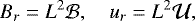 (A.1)
(A.1)
where  is the angular momentum operator and
  and
and  are the poloidal superpotentials that can be expanded in terms of spherical harmonics
  as (Krause & Rädler 1980)
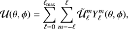 (A.2)
(A.2)
where  are computed as
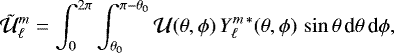 (A.3)
(A.3)
and likewise for  . Owing to the absence of magnetic monopoles, however, there is no contribution to the magnetic field for ℓ = 0. In practice, we work directly with the radial components of velocity and magnetic field, whose transforms are related to
  and
and  via
via  and
and  , respectively.
While testing the decomposition, we noticed that the large-scale field features were fairly well described by the first few modes (0 ≤ ℓ ≤ 5). Therefore, in order to obtain a complete picture, we decompose the magnetic and velocity field in the first eleven spherical harmonics (0 ≤ ℓ ≤ 10) and consider 0 ≤ ℓ ≤ 5 and 0 ≤ m ≤ 5 as the large-scale fields and the rest as small-scale fields. Throughout this work we use the decomposition for the radial velocity and magnetic field on a slice at a fixed radial position of r = 0.98 R.
We illustrate the quality of the reconstruction in Fig. A.1 showing the radial magnetic field from Run La using different numbers of spherical harmonics. In the left panel, the reconstruction was obtained using 1 ≤ ℓ ≤ 10, while in the central panel, the reconstruction is obtained summing over the first 100 spherical harmonics. The right panel shows the original data slice. It is clear from Fig. A.1 that lmax = 10 allows us to capture the main features of the magnetic field and a reasonable amount of the surface total energy (see, Table 4). We show a typical time series of various m-mode energies from the surface radial magnetic field reconstruction of Run Ha in Fig. A.2. This run is dominated by the m = 1 mode, which shows cyclic variations over time, and also long-term changes, during which the axisymmetric modes become comparable to the dominant mode for a short period of time.
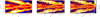 |
Fig. A.1 Spherical harmonic reconstruction, using 1 ≤ ℓ ≤ 10 harmonics (left panel) and 1 ≤ ℓ ≤ 100 harmonics (middle panel), and original data of the radial magnetic field (right panel) near the surface (r = 0.98 R) of Run La. |
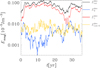 |
Fig. A.2 Time series of the total radial magnetic energy from decomposition (in black) and three of the m modes for Run Ha. Blue: m = 0; red: m = 1; and yellow: small-scale magnetic field. |
References
- Augustson, K., Brun, A. S., Miesch, M., & Toomre, J. 2015, ApJ, 809, 149 [Google Scholar]
- Baliunas, S. L., Donahue, R. A., Soon, W. H., et al. 1995, ApJ, 438, 269 [NASA ADS] [CrossRef] [Google Scholar]
- Beaudoin, P., Simard, C., Cossette, J.-F., & Charbonneau, P. 2016, ApJ, 826, 138 [NASA ADS] [CrossRef] [Google Scholar]
- Berdyugina, S. V., & Tuominen, I. 1998, A&A, 336, L25 [NASA ADS] [Google Scholar]
- Berdyugina, S. V., Pelt, J., & Tuominen, I. 2002, A&A, 394, 505 [NASA ADS] [CrossRef] [EDP Sciences] [Google Scholar]
- Boro Saikia, S., Marvin, C. J., Jeffers, S. V., et al. 2018, A&A, 616, A108 [Google Scholar]
- Brandenburg, A. 2007, IAU Symp., 239, 457 [NASA ADS] [Google Scholar]
- Brandenburg, A., & Giampapa, M. S. 2018, ApJ, 855, L22 [NASA ADS] [CrossRef] [Google Scholar]
- Brandenburg, A., Saar, S. H., & Turpin, C. R. 1998, ApJ, 498, L51 [NASA ADS] [CrossRef] [Google Scholar]
- Brandenburg, A., Mathur, S., & Metcalfe, T. S. 2017, ApJ, 845, 79 [NASA ADS] [CrossRef] [Google Scholar]
- Brown, B. P., Browning, M. K., Brun, A. S., Miesch, M. S., & Toomre, J. 2008, ApJ, 689, 1354 [CrossRef] [Google Scholar]
- Brown, B. P., Browning, M. K., Brun, A. S., Miesch, M. S., & Toomre, J. 2010, ApJ, 711, 424 [Google Scholar]
- Browning, M. K. 2008, ApJ, 676, 1262 [Google Scholar]
- Busse, F. H. 1970, ApJ, 159, 629 [NASA ADS] [CrossRef] [Google Scholar]
- Busse, F. H. 2007, Sol. Phys., 245, 27 [NASA ADS] [CrossRef] [Google Scholar]
- Carroll, T. A., Kopf, M., Strassmeier, K. G., Ilyin, I., & Tuominen, I. 2009, in Cosmic Magnetic Fields: From Planets, to Stars and Galaxies, eds. K. G. Strassmeier, A. G. Kosovichev, & J. E. Beckman, IAU Symp., 259, 437 [NASA ADS] [Google Scholar]
- Chandrasekhar, S. 1961, in Hydrodynamic and hydromagnetic stability (Oxford: Oxford University Press) [Google Scholar]
- Charbonneau, P. 2013, in Solar and Stellar Dynamos, Saas-Fee Advanced Courses (Berlin, Heidelberg: Springer-Verlag), 39, 187 [NASA ADS] [CrossRef] [Google Scholar]
- Chen, C. 1988, in Signal Processing Handbook, Electrical and Computer Engineering (Taylor & Francis) [Google Scholar]
- Cole, E., Käpylä, P. J., Mantere, M. J., & Brandenburg, A. 2014, ApJ, 780, L22 [NASA ADS] [CrossRef] [Google Scholar]
- Distefano, E., Lanzafame, A. C., Lanza, A. F., Messina, S., & Spada, F. 2017, A&A, 606, A58 [NASA ADS] [CrossRef] [EDP Sciences] [Google Scholar]
- Dobler, W., Stix, M., & Brandenburg, A. 2006, ApJ, 638, 336 [NASA ADS] [CrossRef] [Google Scholar]
- Donati, J.-F., & Landstreet, J. D. 2009, ARA&A, 47, 333 [NASA ADS] [CrossRef] [MathSciNet] [Google Scholar]
- Duarte, L. D. V., Wicht, J., & Gastine, T. 2018, Icarus, 299, 206 [NASA ADS] [CrossRef] [Google Scholar]
- Fan, Y., & Fang, F. 2014, ApJ, 789, 35 [NASA ADS] [CrossRef] [Google Scholar]
- Featherstone, N. A., & Hindman, B. W. 2016a, ApJ, 830, L15 [NASA ADS] [CrossRef] [Google Scholar]
- Featherstone, N. A., & Hindman, B. W. 2016b, ApJ, 818, 32 [NASA ADS] [CrossRef] [Google Scholar]
- Gastine, T., Duarte, L., & Wicht, J. 2012, A&A, 546, A19 [NASA ADS] [CrossRef] [EDP Sciences] [Google Scholar]
- Gastine, T., Yadav, R. K., Morin, J., Reiners, A., & Wicht, J. 2014, MNRAS, 438, L76 [NASA ADS] [CrossRef] [Google Scholar]
- Ghizaru, M., Charbonneau, P., & Smolarkiewicz, P. K. 2010, ApJ, 715, L133 [NASA ADS] [CrossRef] [Google Scholar]
- Gizon, L., Duvall, T. L., & Schou, J. 2003, Nature, 421, 43 [NASA ADS] [CrossRef] [PubMed] [Google Scholar]
- Green, C. A., & Kosovichev, A. G. 2006, ApJ, 641, L77 [NASA ADS] [CrossRef] [Google Scholar]
- Hackman, T., Pelt, J., Mantere, M. J., et al. 2013, A&A, 553, A40 [NASA ADS] [CrossRef] [EDP Sciences] [Google Scholar]
- Hackman, T., Lehtinen, J., Rosén, L., Kochukhov, O., & Käpylä, M. J. 2016, A&A, 587, A28 [NASA ADS] [CrossRef] [EDP Sciences] [Google Scholar]
- Hanasoge, S. M., Duvall, T. L., & Sreenivasan, K. R. 2012, Proc. Natl. Acad. Sci., 109, 11928 [Google Scholar]
- Harutyunyan, G., Strassmeier, K. G., Künstler, A., Carroll, T. A., & Weber, M. 2016, A&A, 592, A117 [NASA ADS] [CrossRef] [EDP Sciences] [Google Scholar]
- Hotta, H., Rempel, M., & Yokoyama, T. 2014, ApJ, 786, 24 [NASA ADS] [CrossRef] [Google Scholar]
- Hotta, H., Rempel, M., & Yokoyama, T. 2016, Science, 351, 1427 [NASA ADS] [CrossRef] [Google Scholar]
- Ishihara, N., & Kida, S. 2000, J Phys. Soc. Japan, 69, 1582 [NASA ADS] [CrossRef] [Google Scholar]
- Järvinen, S. P., Korhonen, H., Berdyugina, S. V., et al. 2008, A&A, 488, 1047 [NASA ADS] [CrossRef] [EDP Sciences] [Google Scholar]
- Jetsu, L. 1996, A&A, 314, 153 [NASA ADS] [Google Scholar]
- Jetsu, L., Pelt, J., & Tuominen, I. 1993, A&A, 278, 449 [NASA ADS] [Google Scholar]
- Jones, C. A. 2014, Icarus, 241, 148 [NASA ADS] [CrossRef] [Google Scholar]
- Käpylä, P. J., Mantere, M. J., & Brandenburg, A. 2012, ApJ, 755, L22 [NASA ADS] [CrossRef] [Google Scholar]
- Käpylä, P. J., Mantere, M. J., Cole, E., Warnecke, J., & Brandenburg, A. 2013, ApJ, 778, 41 [NASA ADS] [CrossRef] [Google Scholar]
- Käpylä, P. J., Käpylä, M. J., & Brandenburg, A. 2014, A&A, 570, A43 [NASA ADS] [CrossRef] [EDP Sciences] [Google Scholar]
- Käpylä, M. J., Käpylä, P. J., Olspert, N., et al. 2016, A&A, 589, A56 [NASA ADS] [CrossRef] [EDP Sciences] [Google Scholar]
- Käpylä, P. J., Käpylä, M. J., Olspert, N., Warnecke, J., & Brandenburg, A. 2017, A&A, 599, A5 [Google Scholar]
- Karak, B. B., Käpylä, P. J., Käpylä, M. J., et al. 2015, A&A, 576, A26 [NASA ADS] [CrossRef] [EDP Sciences] [Google Scholar]
- Kitchatinov, L. L., & Rüdiger, G. 1999, A&A, 344, 911 [NASA ADS] [Google Scholar]
- Kővári, Z., Bartus, J., Strassmeier, K. G., et al. 2007, A&A, 474, 165 [NASA ADS] [CrossRef] [EDP Sciences] [Google Scholar]
- Kochukhov, O., Mantere, M. J., Hackman, T., & Ilyin, I. 2013, A&A, 550, A84 [NASA ADS] [CrossRef] [EDP Sciences] [Google Scholar]
- Krause, F., & Rädler, K.-H. 1980, in Mean-field Magnetohydrodynamics and Dynamo Theory (Oxford: Pergamon Press) [Google Scholar]
- Lehtinen, J., Jetsu, L., Hackman, T., Kajatkari, P., & Henry, G. W. 2016, A&A, 588, A38 [NASA ADS] [CrossRef] [EDP Sciences] [Google Scholar]
- Lindborg, M., Mantere, M. J., Olspert, N., et al. 2013, A&A, 559, A97 [NASA ADS] [CrossRef] [EDP Sciences] [Google Scholar]
- Morin, J., Donati, J.-F., Petit, P., et al. 2010, MNRAS, 407, 2269 [NASA ADS] [CrossRef] [MathSciNet] [Google Scholar]
- Moss, D., & Brandenburg, A. 1995, Geophys. Astrophys. Fluid Dyn., 80, 229 [NASA ADS] [CrossRef] [Google Scholar]
- Moss, D., Barker, D. M., Brandenburg, A., & Tuominen, I. 1995, A&A, 294, 155 [NASA ADS] [Google Scholar]
- Nelson, N. J., Brown, B. P., Brun, A. S., Miesch, M. S., & Toomre, J. 2013, ApJ, 762, 73 [NASA ADS] [CrossRef] [Google Scholar]
- Noyes, R. W., Weiss, N. O., & Vaughan, A. H. 1984, ApJ, 287, 769 [NASA ADS] [CrossRef] [Google Scholar]
- Oláh, K., Kolláth, Z., Granzer, T., et al. 2009, A&A, 501, 703 [NASA ADS] [CrossRef] [EDP Sciences] [Google Scholar]
- Oláh, K., Kővári, Z., Petrovay, K., et al. 2016, A&A, 590, A133 [NASA ADS] [CrossRef] [EDP Sciences] [Google Scholar]
- Olspert, N., Käpylä, M. J., Pelt, J., et al. 2015, A&A, 577, A120 [NASA ADS] [CrossRef] [EDP Sciences] [Google Scholar]
- Olspert, N., Lehtinen, J. J., Käpylä, M. J., Pelt, J., & Grigorievskiy, A. 2018, A&A, in press, DOI: 10.1051/0004-6361/201732525 [Google Scholar]
- Ossendrijver, M. 2003, A&A Rev., 11, 287 [NASA ADS] [CrossRef] [Google Scholar]
- Parker, E. N. 1955, ApJ, 121, 491 [NASA ADS] [CrossRef] [Google Scholar]
- Pelt, J., Brooke, J. M., Korpi, M. J., & Tuominen, I. 2006, A&A, 460, 875 [NASA ADS] [CrossRef] [EDP Sciences] [Google Scholar]
- Pipin, V. V. 2017, MNRAS, 466, 3007 [NASA ADS] [CrossRef] [Google Scholar]
- Pulkkinen, P., & Tuominen, I. 1998, A&A, 332, 748 [NASA ADS] [Google Scholar]
- Rädler, K.-H., Wiedemann, E., Brandenburg, A., Meinel, R., & Tuominen, I. 1990, A&A, 239, 413 [NASA ADS] [Google Scholar]
- Reinhold, T., & Gizon, L. 2015, A&A, 583, A65 [NASA ADS] [CrossRef] [EDP Sciences] [Google Scholar]
- Reinhold, T., Reiners, A., & Basri, G. 2013, A&A, 560, A4 [NASA ADS] [CrossRef] [EDP Sciences] [Google Scholar]
- Reinhold, T., Cameron, R. H., & Gizon, L. 2017, A&A, 603, A52 [NASA ADS] [CrossRef] [EDP Sciences] [Google Scholar]
- Roettenbacher, R. M., Monnier, J. D., Korhonen, H., et al. 2016, Nature, 533, 217 [NASA ADS] [CrossRef] [Google Scholar]
- Rosén, L., Kochukhov, O., Hackman, T., & Lehtinen, J. 2016, A&A, 593, A35 [NASA ADS] [CrossRef] [EDP Sciences] [Google Scholar]
- Rüdiger, G. 1978, Astron. Nachr., 299, 217 [NASA ADS] [CrossRef] [Google Scholar]
- Saar, S. H., & Brandenburg, A. 1999, ApJ, 524, 295 [NASA ADS] [CrossRef] [Google Scholar]
- Schrinner, M., Petitdemange, L., & Dormy, E. 2012, ApJ, 752, 121 [NASA ADS] [CrossRef] [Google Scholar]
- See, V., Jardine, M., Vidotto, A. A., et al. 2016, MNRAS, 462, 4442 [NASA ADS] [CrossRef] [Google Scholar]
- Stassun, K. G., Hebb, L., Covey, K., et al. 2011, in 16th Cambridge Workshop on Cool Stars, Stellar Systems, and the Sun, eds. C. Johns-Krull, M. K. Browning, & A. A. West, ASP Conf. Ser., 448, 505 [NASA ADS] [Google Scholar]
- Strugarek, A., Beaudoin, P., Charbonneau, P., Brun, A. S., & do Nascimento J.-D. 2017, Science, 357, 185 [NASA ADS] [CrossRef] [Google Scholar]
- Warnecke, J. 2018, A&A, 616, A72 [NASA ADS] [CrossRef] [EDP Sciences] [Google Scholar]
- Warnecke, J., Käpylä, P. J., Käpylä, M. J., & Brandenburg, A. 2014, ApJ, 796, L12 [NASA ADS] [CrossRef] [Google Scholar]
- Warnecke, J., Käpylä, P. J., Käpylä, M. J., & Brandenburg, A. 2016, A&A, 596, A115 [NASA ADS] [CrossRef] [EDP Sciences] [Google Scholar]
- Warnecke, J., Rheinhardt, M., Tuomisto, S., et al. 2018, A&A, 609, A51 [NASA ADS] [CrossRef] [EDP Sciences] [Google Scholar]
- Weber, M., Strassmeier, K. G., & Washuettl, A. 2005, Astron. Nachr., 326, 287 [NASA ADS] [CrossRef] [Google Scholar]
- Yadav, R. K., Christensen, U. R., Morin, J., et al. 2015a, ApJ, 813, L31 [NASA ADS] [CrossRef] [Google Scholar]
- Yadav, R. K., Gastine, T., Christensen, U. R., & Reiners, A. 2015b, A&A, 573, A68 [NASA ADS] [CrossRef] [EDP Sciences] [Google Scholar]
A video of the surface radial magnetic field evolution of Run La can be found from https://www.youtube.com/watch?v=2g4r1uanrj4.
All Tables
Summary of the transitions from antisolar-like to solar-like differential rotation and between predominantly axisymmetric and nonaxisymmetric large-scale fields from observations and our simulations as a function of increasing Coriolis number.
All Figures
|
Fig. 1 Mollweide projection of radial velocity ur at r = 0.98 R for Runs A2, C3, Ga, H, Ha, and La. |
| In the text | |
|
Fig. 2 Panel a: normalized power spectra P of the radial velocity as function of degree ℓ for Runs A2, C3, Ga, H, La, and Ma with increasing rotational influence. Panel b: degree of peak power ℓpeak estimated from the power spectra plotted over Coriolis number Co. The runs are indicated with their run names. The red dashed line represents a power law fit including all the runs; the blue dashed line represents the fit for the high-resolution runs, while the black dashed line indicates the expected slope from theoretical estimates (Chandrasekhar 1961). |
| In the text | |
|
Fig. 3 Kinetic energy of the decomposition as a function of Coriolis number Co for all 2π runs showing the total energy (panel a), axisymmetric (m = 0, blue), fifth nonaxisymmetric mode (m = 5, red), and small-scale (l, m > 5, orange) contribution (panel b). All the energies in panel b are normalized to the total energy (panel a). Filled circles connected by a continuous line indicate high-resolution runs. |
| In the text | |
|
Fig. 4 Normalized angular velocity Ω(r, θ) of Runs A2, C3, Ga, H, Ha, and La. The dashed lines denote the radius r = 0.98 R, which is used for the further analysis. |
| In the text | |
|
Fig. 5 Relative latitudinal differential rotation |
| In the text | |
|
Fig. 6 Modulus of the absolute latitudinal differential rotation, |
| In the text | |
|
Fig. 7 Radial profiles of the total magnetic energy density Emag averaged over time, latitude, and azimuth for Runs A2, C3, Ga, Ha, La, and Ma. |
| In the text | |
|
Fig. 8 Ratio of total magnetic to kinetic energies Emag∕Ekin as a functionof Coriolis number Co. The red filled symbols (connected by a line) denote high-resolution runs. Blue triangles refer to π∕2 wedge runs. |
| In the text | |
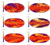 |
Fig. 9 Radial magnetic field Br at r = 0.98 R from the same runs as in Fig. 1. |
| In the text | |
|
Fig. 10 Axisymmetric mean (m = 0, blue) energy vs. nonaxisymmetric large-scale (m = 1, 5; red) energy fraction at the surface (panel a). Axisymmetric mean (m = 0; blue) energy fraction vs. the first nonaxisymmetric mode (m = 1; red) energy fraction (panel b). The dotted black line denotes the axisymmetric to nonaxisymmetric transition at region Co ≈ 3. In both plots, the dashed red and blue lines connect 2π runs; filled symbols, connected with solid lines, denote the high-resolution runs. |
| In the text | |
|
Fig. 11 Mean toroidal magnetic field |
| In the text | |
|
Fig. 12 Ratio of the rotation period to the cycle period as a function of Coriolis number (panel a). The two black lines indicate the fit to the axisymmetric and rapid rotation runs, respectively. The vertical lines denote the nonaxisymmetric transition found in our simulations (dotted; Co ≥ 3) and from the observational study of Lehtinen et al. (2016) (dashed), respectively. Runs are plotted after their labels. The color indicates the mode chosen for calculating τcyc: blue for m =0, red for m = 1. Prot ∕Pcyc as function of activity, represented by Emag∕Ekin is shown in panel b. Panel c: comparison between the results presented in this paper, Lehtinen et al. (2016), and Strugarek et al. (2017). Black circles and triangles denote high resolution and π∕2 wedges in our set, respectively. The gray dots indicate M dwarfs and F and G stars from Brandenburg et al. (2017). |
| In the text | |
|
Fig. 13 Reconstruction of the m = 1 mode of the magnetic field at the surface of the star for Runs C3, Ga, Ha, and La at θ = +60°. The black and white line indicates the path due to differential rotation alone. |
| In the text | |
|
Fig. 14 Standing dynamo wave of Run La. Lower panel: time variation of the four regions indicated in the upper panel. |
| In the text | |
|
Fig. 15 Upper panel: flip-flop for Run J. The dashed line is the differential rotation at θ = +45°. Lower panel:same as Fig. 13, but at θ = +45°, for Run Ga. The ADW has been de-migrated to better show the active longitudes. |
| In the text | |
|
Fig. A.1 Spherical harmonic reconstruction, using 1 ≤ ℓ ≤ 10 harmonics (left panel) and 1 ≤ ℓ ≤ 100 harmonics (middle panel), and original data of the radial magnetic field (right panel) near the surface (r = 0.98 R) of Run La. |
| In the text | |
|
Fig. A.2 Time series of the total radial magnetic energy from decomposition (in black) and three of the m modes for Run Ha. Blue: m = 0; red: m = 1; and yellow: small-scale magnetic field. |
| In the text | |
Current usage metrics show cumulative count of Article Views (full-text article views including HTML views, PDF and ePub downloads, according to the available data) and Abstracts Views on Vision4Press platform.
Data correspond to usage on the plateform after 2015. The current usage metrics is available 48-96 hours after online publication and is updated daily on week days.
Initial download of the metrics may take a while.