© ESO 2018

1 Introduction

With the aim of using an improved method to study the dynamics of galaxy pairs, we constructed two new pair catalogs using well-defined criteria and improved observational data. The first is a catalog of ≈1000 pairs with high accuracy radial velocities (Chamaraux & Nottale 2016) extracted from Nilson’s Uppsala Galaxy Catalog (UGC; Nilson 1973), which has the advantage that it is complete in apparent diameter. The second is a catalog of ≈13 000 pairs (Nottale & Chamaraux 2018, the largest presently available to our knowledge), which makes use of the huge recent increase in astronomical data. We used the HyperLEDA database (2016, Makarov et al. 2014) to identify galaxy pairs and extract their parameters from the large surveys (e.g., SDSS; Alam et al. 2015 and 2MASS).

To improve our understanding of physics at extragalactic scales, the goal of this paper is to elaborate better methods of statistical analysis of galaxy pair data (which can also be applied to any type of pairs of astronomical objects). This is the goal of the present paper. We need to obtain statistical information on the physical characteristics of these pairs, particularly their masses through Kepler’s third law and the possible existence of anomalous dynamics in these pairs. Such a new dynamics is, according to various proposals, attributed to missing mass or dark matter (Bergstrom 2000), to modification of gravity (Sanders 2002), or to a new dark potential (Nottale 2011; Chavanis 2017a,b).

In order to compute those physical quantities, we have to know the 3D velocity difference between the pair members and their 3D interdistances. But we have at our disposal only one component of the velocity difference (along the line of sight) and two components of the interdistance (projection on the sky-plane). Therefore one has to find statistical methods to obtain those 3D quantities from the projected quantities. We call these methods statistical deprojection. Moreover, we note that for each galaxy pair we can determine the various 3D parameters for only one point of each galaxy orbit and only one instant.

Because of these limitations, various methods of analysis have been devised (Chengalur et al. 1996; Peterson 1979; Faber & Gallagher 1979). However, as shown by Faber & Gallagher (1979), these methods remain unsatisfactory from a mathematical viewpoint. In particular, recovering the mass remains very uncertain. For these reasons, we propose new methods of deprojection, which we show here to yield more precise results for recovering the 3D unprojected parameters.

The paper is organized as follows. In Sect. 2 we first analyze the statistical projection process and derive the probability distributions expected for the various relevant projected quantities, namely, intervelocity, v_z; interdistance, r_p; their ratio, r_p ∕v_z, which can be used as signature of circular orbits; and the product, $r_p{v}_z^2$, which is involved in mass determination.

In Sect. 3, we develop statistical methods of deprojection of these parameters, that is, intervelocity, interdistance, and mass, based on the previous analysis. We start from a histogram of the projected data organized in various ways, i.e., constant bins, moving bins, and variable moving bins. Then we apply inversion formulae, which amount in some cases to matrix inversion, to obtain the deprojected distributions. Finally we test these methods using numerical simulations, which also allow us to determine the uncertainties involved.

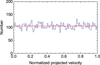Fig. 1 Theoretical expectation vs. numerical simulation of the statistical distribution of vz ∕v, where vz is the radial velocity difference between galaxies in randomly oriented pairs and v the true velocity difference. The number of simulated pairs is here N ≈ 10 000. Apart from statistical fluctuations, the obtained probability distribution of the radial velocity is constant in the range [0, v], in agreement with the theoretical expectation (given by the constant red line).

2 Statistical analysis

Let us use a cylindrical coordinate system whose axis z is oriented from the observer to the galaxy pair. In this case the (x, y) plane is the plane of the sky. The position vector r is defined as $$x=r_p\cos \phi ,y=r_p\sin \phi ,z,$$(1)

while the velocity vector v is defined as $$v_x=v_p\cos {\phi }_v,v_y=v_p\sin {\phi }_v,v_z.$$(2)

The measured quantities are the position vector projected on the plane of the sky, r_p = (x, y), and the radial velocity v_z. Then r_p, v_z, and φ are known while z, v_p, and φ_v are unknown variables.

2.1 Probability distribution of radial velocity

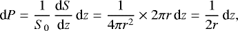
Consider a randomly oriented 3D vector (x, y, z) of fixed length r. Let us determine the probability distribution of any of its projections, say z. The part of the sphere of radius r which projects between z and z + dz has a surface $$\text{d}S=-2\pi r_{p}r\text{\hspace{0.17em}d}\theta =-2\pi r^2\sin \theta \text{\hspace{0.17em}d}\theta =\frac{\text{d}S}{\text{d}z}\text{d}z.$$(3)

Since z = rcosθ, then d z = −rsinθ dθ, and we finally find that dS∕dz = 2πr. The probability distribution of the projection on any axis of a randomly oriented 3D vector of length r can then be derived $$\text{d}P=\frac{1}{S_0}\frac{\text{d}S}{\text{d}z}\text{\hspace{0.17em}d}z=\frac{1}{4\pi r^2}\times 2\pi r\text{\hspace{0.17em}d}z=\frac{1}{2r}\text{\hspace{0.17em}d}z,$$(4)

and it is therefore constant when r is constant. Since z can vary from − r to + r, we verify that this probability distribution is correctly normalized.

This can be easily applied to the velocity vector. Given a fixed pair configuration (r, v) with random orientation, the probability distribution of the values of the radial velocity differences between the pair members is 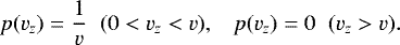$$p(v_z)=\frac{1}{v}(0<v_z<v),p(v_z)=0(v_z>v).$$(5)

We note that here no member of the pair is priviledged, such that we consider only positive differences, which then vary between 0 and v.

We performed a numerical simulation of this projection of a given pair with random orientation. The obtained distribution of v_z confirms this expectation (Fig. 1).

2.2 Probability distribution of projected distance

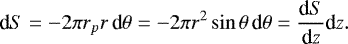
We consider a pair of objects, the 3D interdistance between which is r, fixed. Let $r_p=\sqrt{x^2+y^2}$ be the distance between the pair members projected on the plane of the sky. The part of the sphere corresponding to projected distances lying in the interval [r_p, r_p + dr_p] is made of two rings of width rdθ and radius r_p. Therefore its surface isdS = 4πr_prdθ. Now, since r_p = rsinθ, we find $$\text{d}\theta =\frac{\text{d}{r}_p}{\sqrt{r^2-r_p^2}}.$$(6)

The differential probability distribution of r_p is d P = dS∕(4πr²). Then the normalized probability density of r_p values p(r_p), projected from a given r value, is written as $$p(r_p)=\frac{\text{d}P(r_p)}{\text{d}{r}_p}=\frac{r_p}{\sqrt{r^2-r_p^2}}.$$(7)

We performed a numerical simulation of such a projection. The obtained distribution is in fair agreement with this theoretical expectation (Fig. 2).

More generally, we consider now a set of pairs whose distances between their members are distributed with a probability P_r (r) when r lies in the interval [r₁, r₂]. When the pair orientation is random, the expected probability distribution of the projected distances on the plane of the sky is now given by $$p(r_p)={\displaystyle {\int }_{r_1}^{r_2}\frac{P_r(r)r_p\text{\hspace{0.17em}d}r}{r\sqrt{r^2-r_p^2}}}.$$(8)

2.3 Probability distribution of ratio ζ = r_p∕v_z

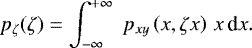
This ratio can be used as signature of circular orbits. We give in Appendix A the probability distribution of a product and of the ratio of two variables, of which the individual probability distributions are known, and also that of the inverse of a variable. From these basic formulae, one can infer the probability distribution functions (PDFs) of various combinations of the variables observed for pairs [v_z and (x, y), involving r_p].

Since $p(r_p)=r_p/\sqrt{1-r_p^2}$ with 0 < r_p < 1 (for r = 1) and p(v_z)= 1 with 0 < v_z < 1 (for v = 1), we obtain for the ratio ζ = r_p∕v_z [more generally, ζ = (r_p∕r)∕(v_z∕v)] $$p_{\zeta }(\zeta )={\displaystyle {\int }_0^1{p}_{v_z}}(v_z)p_{r_p}(\zeta v_z)v_z\text{\hspace{0.17em}d}{v}_z,$$(9)

which is written as $$p_{\zeta }(\zeta )={\displaystyle {\int }_0^1\frac{v_z^2\text{\hspace{0.17em}d}{v}_z}{\sqrt{(1/{\zeta }^2)-v_z^2}}}.$$(10)

Two cases must now be considered. When ζ > 1, the integration interval is reduced to [0, 1∕ζ]. One finds 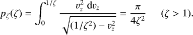$$p_{\zeta }(\zeta )={\displaystyle {\int }_0^{1/\zeta }\frac{v_z^2\text{\hspace{0.17em}d}{v}_z}{\sqrt{(1/{\zeta }^2)-v_z^2}}}=\frac{\pi }{4{\zeta }^2}(\zeta >1).$$(11)

When ζ < 1, the integration interval is again [0, 1] and one finds $$p_{\zeta }(\zeta )=\frac{1}{2}\left[\frac{1}{{\zeta }^2}\arctan \left(\frac{\zeta }{\sqrt{1-{\zeta }^2}}\right)-\frac{\sqrt{1-{\zeta }^2}}{\zeta }\right](\zeta <1).$$(12)

We performed a numerical simulation of randomly oriented pairs with uncorrelated randomly oriented velocity differences. As can be seen in Fig. 3, the theoretically expected distribution agrees very well with the simulation.

In the case of circular orbits, once r_p is given, the possible values of v_z, instead of being uniformly distributed between 0 and v, are constrained to be smaller than v × (r_p∕r). As a consequence, the left part of the PDF of ζ = (r_p∕r)∕(v_z∕v) below ζ = 1 is expected to be empty, which achieves a possible statistical signature of circular orbits.

The probability distribution of the reverse function, χ = v_z∕r_p is easy to derive from these expressions and from Eq. (A.3). We find $$\begin{array}{lll}\hfill & p_{\chi }(\chi )\hfill & =\frac{\pi }{4}(\chi <1),\hfill \\ \hfill & p_{\chi }(\chi )\hfill & =\frac{1}{2}\left[\arctan \left(\frac{1}{\sqrt{{\chi }^2-1}}\right)-\frac{\sqrt{{\chi }^2-1}}{{\chi }^2}\right](\chi >1).\hfill \end{array}$$

It is therefore constant up to χ = 1, after which it decreases quickly toward 0. In the case of circular orbits, only the constant part of the PDF remains (0 < χ < 1), which means that the projection of v_z∕r_p becomes similar to that of v_z.

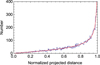Fig. 2 Numerical simulation of the probability density distribution of rp∕r, where rp is the projection on the plane of the sky of the distance r between members of randomly oriented pairs (for a fixed 3D r value). The number of simulated pairs is N ≈ 10 000. Apart from statistical fluctuations, the obtained probability distribution agrees with the theoretical expectation (continuous red line, see text).

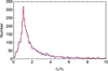Fig. 3 Numerical simulation of the density distribution of the ratio rp∕vz, where rp is the distance between pair members projected on the plane of the sky and vz is their radial velocity difference (here with r = 1 and v = 1). The number of simulated pairs is N = 4000. Within statistical fluctuations, the obtained probability distribution agrees well with the theoretical expectation (red continuous line, Eqs. (11) and (12)). In the case of circular orbits, the velocity and radial vectors are orthogonal, which implies rp ∕vz ≥ r∕v (see text), i.e., rp∕vz ≥ 1 in this figure. That achieves a clear signature of circular orbits, for which the left part of the figure (rp ∕vz < 1) below the sharp peak of the rp∕vz PDF is expected to be empty.

2.4 Probability distribution of product $\eta =r_p{v}_z^2$

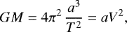
This product is involved in mass determination. Indeed, the orbits of isolated galaxy pairs are subjected to Kepler’s third law, 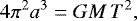$$4{\pi }^2{a}^3=GM{T}^2,$$(15)

where M = M₁ + M₂, a is the semimajor axis of the orbit and T the period. Defining a characteristic velocity V = 2πa∕T, it yields the total mass of the system 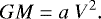$$GM=a{V}^2.$$(16)

The perimeter of an ellipse varies between 4a (radial free fall) and 2πa (circular orbit). This perimeter is given by elliptic integrals, which can be approximated by a power series 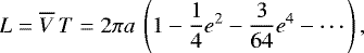$$L=\overline{V}T=2\pi a\left(1-\frac{1}{4}{e}^2-\frac{3}{64}{e}^4-\cdots \right),$$(17)

where e is the eccentricity of the ellipse, and therefore the average velocity $\overline{V}$ is such that $(2/\pi )V<\overline{V}<V$.

When the orbit is circular, r = a and v = V, such that in this case the total mass is given by $$GM=r{v}^2.$$(18)

Instead of r we have only access to r_p, and, instead of v, to v_z. This leads us to look for the probability distribution of $\eta =r_p{v}_z^2$.

Let us set $U=v_z^2$, then $p_U(U)=1/(2\sqrt{U})$, while we recall that $p(r_p)=r_p/\sqrt{1-r_p^2}$ when the radius is normalized to r = 1.

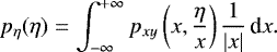
In the case of uncorrelated values of r and v, the general formula for the probability distribution of a product Eq. (A.1) then yields 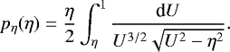$$p_{\eta }(\eta )=\frac{\eta }{2}{\displaystyle {\int }_{\eta }^1\frac{\text{d}U}{U^{3/2}\sqrt{U^2-{\eta }^2}}}.$$(19)

The integration limits are determined by the fact that 0 < v_z < 1 (for a normalized velocity v = 1) and hence U < 1; U² − η² must be > 0 due to the square root such that U > η. This integral can be integrated in terms of the hypergeometric function ₂ F₁ (a, b;c;z) as follows: 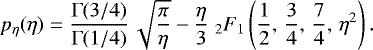$$p_{\eta }(\eta )=\frac{\Gamma (3/4)}{\Gamma (1/4)}\sqrt{\frac{\pi }{\eta }}-\frac{\eta }{3}{}_2{F}_1\left(\frac{1}{2},\frac{3}{4},\frac{7}{4},{\eta }^2\right).$$(20)

This formula is in excellent agreement with the result of a numerical simulation of the projections of r to r_p and v to v_z (Fig. 4).

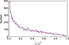Fig. 4 Analytical formula (see text) vs. numerical simulation of the density distribution of the product $r_p{v}_z^2$, where rp is the distance between pair members projected on the plane of the sky and vz is their radial velocity difference. This combination of variable is essential for the statistical determination of the total mass of the pair. The product is plotted here for r = 1 and v = 1, i.e., the plotted variable is actually $(r_p/r){(v_z/v)}^2$. The number of simulated pairs is N ≈ 10 000. Within statistical fluctuations, the obtained probability distribution agrees well with the theoretical expectation (red line, Eq. (20)).

3 Methods of statistical deprojection

The knowledge of the expected statistical distribution of the various variables or of their combination allows one to construct methods of deprojection from the observed subset of variables.

3.1 Deprojection of x, y, and v_z

3.1.1 Theoretical deprojection of v_z

The simplest method of deprojection deals with the value of a vector projected on a single axis. This is the case in particular for v_z (radial velocity difference). The various methods described in this work are also valid for deprojection of the individual observed variables x and y (projections of r on the plane of the sky along right ascension and declination).

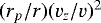
We have seen that, in this case, the expected probability distribution for a random orientation and a given value of the unprojected variable is constant. Therefore, if P_v (v) is the probability distribution of the 3D velocity v, the probability distribution of v_z is given by Nottale (2011) $$P_{v_z}(v_z)={\displaystyle {\int }_{v_z}^{\infty }\frac{P_v(v)}{v}}\text{\hspace{0.17em}d}v.$$(21)

This distribution can be easily inverted. One obtains a deprojection formula, that is, $$P_v(v)=-v{\left[\frac{\text{d}{P}_{v_z}(v_z)}{\text{d}{v}_z}\right]}_v,$$(22)

and similar formulae for x and y separately; the deprojection of their combination in $r_p=\sqrt{x^2+y^2}$ is considered in the following.

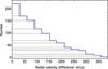Fig. 5 Illustration of the deprojection method for radial velocity (or any 1D variable projected from a 3D vector). For a bin (V i−1, V i) of width δV, where V i = i × δV, Ni is the number of values contained in this bin in the histogram of the projected quantity. The number of objects that have a deprojected value v = V i is given by the area of the rectangle of height (Ni − Ni+1) and of extent [0, V i].

3.1.2 General algorithm of deprojection of v_z

The simplest way to achieve statistical deprojection of a single variable, such as the radial velocity v_z, consists of directly implementing Eq. (22). This formula means that if N_v pairs have a true velocity difference v, their radial velocities are uniformly distributed between 0 and v. The existence of these N_v objects at velocity v creates a jump δN = N_v in the observed distribution of v_z, N(v_z) = N_totP(v_z). Therefore, the contribution of a particular true intervelocity v to the observed PDF of v_z is given by the surface of the rectangle of sides v × δN (see Fig. 5).

3.1.3 Various methods of deprojection of v_z

Differences on adjacent constant bins. The simplest way to implement Eq. (22) consists of

• (1)

  constructing the histogram $N_i^p$ of radial (projected) velocities V _r in bins [V _i−1, V _i] of given width δV;

• (2)

  computing the differences $(N_i^p-N_{i-1}^p)$ between the numbers in successive bins;

• (3)

  multiplying by the rank i = V _i∕δV of the bin.

We obtainedin this way the deprojected numbers, N = V (δN^p∕δV), i.e., in terms of the elements of the histogram, $N_i=i\times (N_i^p-N_{i-1}^p)$. This numbershould be assigned to a bin of width δV and of mean deprojected velocity $V=(i+\frac{1}{2})\delta V$. Indeed, the projected velocity V _i = i δV is the limit between the bins of ranks i and i + 1 in the projected histogram, and the resulting N_i should be assigned to this velocity V _i in the mean, i.e., to a bin centered on this velocity and therefore shifted by δV∕2 with respect to the initial histogram.

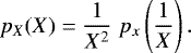
We performed a numerical simulation in which we calculated the mean and standard deviations of 100 realizations of the deprojection (see Fig. 6). We recovered in these simulations the overall shape of the initial distribution (chosen to be a Gaussian of mean 190 km s⁻¹ and standard deviation 90 km s⁻¹). In particular the existence and position of the main peak is recovered in a satisfactory way. We can see in Fig. 6 the improvement obtained when going from a catalog of ≈ 1000 pairs to ≈ 10 000, regarding the decrease of both the optimal bin width and dispersion of the various PDFs. A given realization of a catalog deprojection is expected to be contained (with a high probability) between the two ± 1σ lines, as supported by an example given in Fig. 7 (left part).

However, Eq. (22) presupposes a strictly monotonic decreasing distribution. Otherwise it may lead to obtainingnegative numbers. The problem is that there are fluctuations that may locally break this expected monotony.

For large enough bin sizes, it is clear that the monotony is preserved. Therefore, a possible way to solve this difficulty without losing too much resolution in the deprojection is to choose the smallest of these large enough bins. This value depends on the total number of pairs. In our numerical simulations, the optimal bin width was found to be ≈ 30 km s⁻¹ for ≈1000 pairs and ≈ 20 km s⁻¹ for ≈10 000 pairs.

Another possible method consists of correcting the negative numbers by substracting these numbers to the adjacent bins. This method is possible only for small deviations and reveals to be equivalent to the previous method.

Differences between constant intervals separated by two bins. Actually, the previous method where the difference is taken between two adjacent bins is not optimized and it can therefore be improved. It is more efficient (as in finite difference methods) to take differences between two intervals separated by one bin, $N_{i+1}^p-N_{i-1}^p$. This improvement is based on thefact that f(x + dx) − f(x) = f′(x)dx + O(dx²), while (f(x + dx) − f(x −dx))∕2 = f′(x)dx + O(dx³).

We checked the method by a numerical simulation (see right Fig. 7). We find that the ± 1σ standard deviation on the PDF is half that obtained with the previous method (differences $N_i^p-N_{i-1}^p$), thus achieving a significant improvement.

Differences on constant moving bins. The method that uses constant bins has drawbacks: the result isdigitalized too much, has low resolution, and is too dependent on limits between bins.

Then we devised another method that deals with more information about the original radial velocity PDF and is more continuous. It amounts to performing a histogram of the projected velocities on a large enough moving bin w_bin shifted by a low value, e.g., δv = 1 km s⁻¹. We obtain a function that is both monotonous and quasi-continuous. An example of such a function is given in Fig. 8: it is obtained from the projection of ≈ 12 000 velocities having a Gaussian distribution of mean 150 km s⁻¹ and standard deviation 50 km s⁻¹.

Then we applied on this function the deprojection formula $P_v\text{\hspace{0.22em}d}{v}_r=-V\text{d}{P}_{v_r}$ (Eq. (22)), but with thesmall shift dv_r = δv. Then we performed a moving average of the resulting distribution using the original bin width w_bin.

Numerical simulations were achieved to validate the method. We first defined a given PDF of the 3D velocity v, performed a random realization of this PDF on N_v values v_i, randomly projected them to v_ri, and then we deprojected the distribution obtained using the moving bins method. The process was repeated N_s times to obtain the convenient statistics of the method.

We give in Fig. 9 the results obtained for an initial v distribution showing one unique peak described by a Gaussian for two different peak widths. The quality of the result depends on the width ofthe initial peak: for a large enough peak (left Fig. 9 and Fig. 10), the position, amplitude, and width of the peak are correctly recovered. When the peak is narrower (right Fig. 9), its position is correctly recovered by the deprojection, but its amplitude is slightly too low and correspondingly its width becomes too large (but only within one sigma).

Differences on varying moving bins. In order to account for this bias, we devised another more accurate method. The problem is that, when there is a peak in the PDF of the 3D true velocity v, it manifestsas a high value of the slope in the PDF of the radial (projected) velocity v_r. If the binwidth is too large, this slope is decreased by the smoothing out effect of the binning. As a consequence, the amplitude of the deprojected peak is too low. Thus we corrected this bias by using a moving bin of variable width, decreasing when the slope increases. A balance should be found for the variation of the binwidth, since a smaller bin also increases the fluctuations and therefore the final dispersion. This method gives very good results, since it allows us to recover multiple peaks present in the initial 3D distribution, as can be seen in Fig. 11.

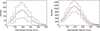Fig. 6 Numerical simulation of the intervelocity deprojection of a sample of 1200 pairs (left figure) and 13 000 pairs (right figure). The original 3D velocities have a Gaussian distribution of standard deviation σv = 90 km s−1 and peak velocity 190 km s−1 (cutoff on V = 0) [red curve]. We randomly project a random realization of this Gaussian distribution, then deproject it using the constant bin method with a bin of width 30 km s−1 (left figure) and 20 km s−1 (right figure, see text). The blue histogram is the mean result of 100 realizations of such a projection/deprojection and the black lines are the ± 1σ lines.

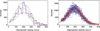Fig. 7 Various realizations of the numerical simulation of the intervelocity deprojection (sample of 13 000 pairs). Left figure: an example of a single realization. The original 3D velocities have a Gaussian distribution of standard deviation σv = 90 km s−1 and peak velocity 190 km s−1 (cutoff on V = 0) [red curve]. We randomly projected a random realization of this Gaussian distribution, then deprojected it using the constant bin method with a bin width 20 km s−1 (see text). The blue broken line is the obtained deprojection, compared with the ± 1σ lines estimated from 100 realizations (see Fig. 6). Right figure: various realizations using differences on non-adjacent bins ($N_{i+1}^p-N_{i-1}^p$), for the same original velocity PDF. We randomly projected random realizations of this Gaussian distribution, then deprojected it using the constant bin method (blue histograms) with a bin width 20 km s−1 (see text). The dashed orange lines show the ± 1σ lines estimated from 100 realizations. The quality of the deprojection is improved by a factor of ≈ 2 with respect to the adjacent bin method.

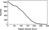Fig. 8 Histogram of the projected velocities (from an initial Gaussian distribution of mean 150 km s−1 and standard deviation 50 km s−1) on a moving bin wbin shifted by differences between bin positions δv = 1 km s−1.

3.2 Deprojection of r_p

3.2.1 Theoretical deprojection

Although one can obtain the probability distribution of r from x and y separately, more information is contained in their combination 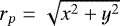$r_p=\sqrt{x^2+y^2}$, from which a better deprojection is expected to be achieved. This expectation is confirmed by the distribution of r_p for a given value of r, which shows a strong peak at r_p = r (Fig. 2). Assuming a probability distribution P_r(r) of the unprojected variable r, one expects for r_p a probability distribution, i.e., 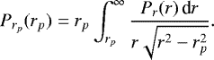$$P_{r_p}(r_p)=r_p{\displaystyle {\int }_{r_p}^{\infty }\frac{P_r(r)\text{\hspace{0.17em}d}r}{r\sqrt{r^2-r_p^2}}}.$$(23)

For example, if the unprojected probability distribution is constant between 0 and r₀, the projected distribution is given by (see Fig. 12) $$P_{r_p}(r_p)=\arccos \left(\frac{r_p}{r_0}\right).$$(24)

It does not seem possible to invert this formula analytically. However, it is very possible to construct an algorithm to perform this inversion numerically.

3.2.2 Deprojection method for r_p

Let i_max be the total number of bins in the histogram of r_p values. We denote $N_i^p$ the observed number of projected values r_p in the bin of rank i. This number is the sum of contributions of 3D values r ≥ r_p from bins of rank j ≥ i – we assume a same number of bins for the r and r_p histograms (see Fig. 12).

Let us derive the probability law for the various contributions. The probability distribution of r_p for a given r value has been shown (Sect. 2.2) to be $$p(x)=\frac{x}{\sqrt{1-x^2}},$$(25)

for x = r_p∕r. We assume, as an approximation valid for a small enough bin width (i.e., a large enough number of bins), that the probability distribution of r remains constant in any bin. Then the probability density of given r values projected in the bin of rank i and relative width b is written as $$p_{bi}={\displaystyle {\int }_{b(i-1)}^{bi}\frac{x}{\sqrt{1-x^2}}}\text{\hspace{0.17em}d}x=\sqrt{1-b^2{(i-1)}^2}-\sqrt{1-b^2{i}^2}.$$(26)

Concerning the r values pertaining to the bin of rank j, the normalized x values (i.e., r_p ≤ r) belong to only a total number of j bins, such that the relative bin width (normalized to a total range x = 0 to 1) is b = 1∕j.

Let us now show that the probability law of the contributions of the various r values (given by index j) can be recovered from that of the projected values r_p (given by index i).

Indeed, let us introduce the matrix $${\pi }_{ij}=\sqrt{1-{\left(\frac{i-1}{j}\right)}^2}-\sqrt{1-{\left(\frac{i}{j}\right)}^2},$$(27)

for i≤ j. The other elements of this matrix (i > j) are zero. Let P_ij be the transpose of this matrix, i.e., P = π^T.

If the column vector $N_i^p$ represents the various projected numbers in the bin of rank i, they are obtained from the initial 3D column vector $N_j^r$ by the matrix product 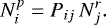$$N_i^p=P_{ij}{N}_j^r.$$(28)

Therefore the initial unprojected probability distribution is recovered from a mere matrix inversion, i.e., $$N_j^r=P_{ji}^{-1}{N}_i^p.$$(29)

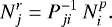
For example, for three bins the relation between the probability distributions is written as $$\begin{array}{ll}{N}_1^p\hfill & =1.000N_1^r+0.134N_2^r+0.057N_3^r,\hfill \\ N_2^p\hfill & =0.000N_1^r+0.866N_2^r+0.197N_3^r,\hfill \\ N_3^p\hfill & =0.000N_1^r+0.000N_2^r+0.745N_3^r.\hfill \end{array}$$

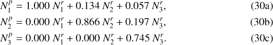
The deprojected reverse relation is, in this case, $$\begin{array}{ll}{N}_1^r\hfill & =1.000N_1^p-0.155N_2^p-0.036N_3^p,\hfill \\ N_2^r\hfill & =0.000N_1^p+1.155N_2^p-0.306N_3^p,\hfill \\ N_3^r\hfill & =0.000N_1^p+0.000N_2^p+1.342N_3^p.\hfill \end{array}$$

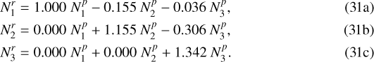
This method is illustrated in Fig. 13, where we deproject a projected distribution N_p = arccosr_p, which is the expected function for a constant initial distribution N_r = cst (in the null bin width limit). The deprojected distribution is constant as expected, except for a small bias mainly involving the first and last bins (which is therefore easy to correct and disappears when the number of bins is increased). Another example is given in the numerical simulation of Fig. 14, where the initial 3D distribution is randomly drawn from a Gaussian probability density (10 000 points). This distribution is nicely recovered from the matrix inversion method. In this case the bias involving the extreme points is unobservable, since these values are almost vanishing.

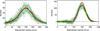Fig. 9 Deprojections by constant moving bins method of several realizations of a sample projected from an initial Gaussian distribution (Nv ≈ 1200 points, Ns = 25 realizations). We show the mean deprojected distribution (black curve) and the ± 1σ limits (green curves) compared with the initial distribution (red curve). In the left figure, the peak position is 150 km s−1 and its standard deviation 50 km s−1. The deprojection shows no bias with such a velocity peak width. In the right figure, the peak position is 150 km s−1 and the standard deviation 20 km s−1. The deprojection shows a bias with such a narrow velocity peak width. The deprojected velocity peak is too low by ≈ 12% and too wide by ≈20%, although the peak position is precisely recovered to within ≈1%.

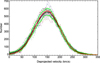Fig. 10 Deprojections by the constant moving bins method of several realizations of a sample projected from an initial Gaussian distribution with peak position 150 km s−1 and standard deviation 50 km s−1 (Nv ≈ 12 000 points, Ns = 25 realizations). We show the mean deprojected distribution (black curve) and the ± 1σ limits (greencurves) compared with the initial distribution (red curve). The quality of the deprojection is clearly improved compared to the 1200 points case, in particular concerning the peak amplitude (Fig. 9).

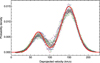Fig. 11 Deprojection by a varying moving bin. The bin width varies between 20 and 40 km s−1 dependingon the slope. The obtained distribution is finally smoothed out by a bin width 20 km s−1. We performed several realizations of a sample projected from an initial two-Gaussian peaks distribution with respective peak positions 70 and 150 km s−1 and standard deviations 15 and 20 km s−1 (Nv ≈ 12 000 points, Ns = 25 realizations). We show the initial distribution as a red continuous curve. Despite the narrowness of the peaks, the quality of the deprojection is very good since the two peaks and the intermediate hollow are clearly identified at their true positions.

3.3 Deprojection of mass

3.3.1 Theoretical deprojection

The total mass M = M₁ + M₂ of a pair of objects in relative Keplerian motion is given by $$GM=4{\pi }^2\frac{a^3}{T^2}=a{V}^2,$$(32)

where G is Newton’s constant of gravitation, a is the semimajor axis of the orbit of one object around the other, and T is the periodand V = 2πa∕T.

However, there are two drawbacks that deteriorate the available information on mass, since we have no direct access to a and V: first, we deal only with instantaneous interdistance r and velocity v; and second these 3D values are themselves projected to r_p and v_z, i.e., $a{V}^2\to r{v}^2\to r_p{v}_z^2$. The first drawback vanishes for circular orbits, but it can lead to some additional uncertainty in the elliptical case, since the relation between M and rv² is written as $$r{v}^2=GM(1+e\cos \xi ),$$(33)

where e is the eccentricity and ξ the parameter of the orbit, which is such that r = a(1 − ecosξ) and t = (T∕2π)(ξ − esinξ). The value of rv²∕GM fluctuates between 1 − e and 1 + e while its time average varies from 1 to 0.5 when e varies from 0 to 1, respectively; it can be approximated by the relation ⟨rv² ⟩∕GM = cos²(πe∕4) up to some percents.

The mass distribution should therefore be statistically deprojected from the observed products $r_p{v}_z^2$. We established in Sect. 2.4 the expected PDF of the projection of a given value of rv² (see Eq. (20) and Fig. 4).

From this formula, one can theoretically deproject any distribution of $r_p{v}_z^2$. Its analytical integration does not seem to be possible, but, as in the case of the deprojection of r_p, it is very possible to construct an algorithm to perform this inversion numerically. However, this deprojection is expected to be difficult, since the individual projection function vanishes for the original unprojected value rv² (see Fig. 4), while it is constant for v_z (easier deprojection) and shows a divergent peak for r_p (best deprojection).

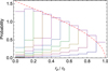Fig. 12 Illustration of the method of deprojection of rp, for 10 bins and an initial distribution Pr(r) = constant between 0 and r0. We show how the initial unprojected number density in each given bin (this initial density is chosen to be constant = 1) is distributed among the original bin and those at smaller distances (areas contained between the broken lines). The red dashed line is the expected distribution [arccos(rp)] in the limit of vanishing bin width (infinite number of bins). Conversely, one can recover the initial unprojected distribution from the projecteddistribution by inverting such a decomposition (see text). There is just a small bias on the first and last bins.

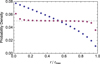Fig. 13 Example of statistical deprojection of rp for a constantPDF of r. We start froma projected distribution Np = arccos(rp) (inclined blue points) for 20 bins (see text). The deprojected probability distribution is shown as almost horizontal magenta points.

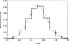Fig. 14 Example of deprojection of rp for a projected distribution Np obtained from a 3D (unprojected) initial Gaussian distribution Nr (black histogram, total 10 000 points) for 10 bins. The deprojected probability distribution (magenta points) is in good agreement with the initial probability distribution.

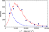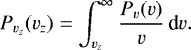
Fig. 15 Example of deprojection (points) of a projected distribution $r_p{v}_z^2$ (decreasing blue curve) obtained from a 3D (unprojected) initial distribution r v2 (red curve), for 10 bins. The initial distribution is built from a Gaussian velocity distribution of mean 200 km s−1 and dispersion 50 km s−1 and a Gaussian distance distribution of mean 0.3 Mpc and dispersion 0.05 Mpc.

3.3.2 Deprojection method for $r_p{v}_z^2$

As in the deprojection method for r_p, let us introduce a projection matrix constructed from the projection function p_η (η) given in Eq. (20) and Fig. 4. We divide the η range into N bins. The projection matrix is written as (for its non-null coefficients) 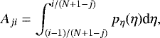$$A_{ji}={\displaystyle {\int }_{(i-1)/(N+1-j)}^{i/(N+1-j)}{p}_{\eta }}(\eta )\text{d}\eta ,$$(34)

where j = 1 to N and i = 1 to N + 1 − j (and A_ji = 0 for the remaining coefficients).

Then the deprojection matrix is obtained from this matrix by the following transformation: $$B=\text{Reverse}[\text{Inverse}[\text{Transpose}[\text{A}]]].$$(35)

For example, for N = 3, the projection matrix is written as 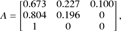$$A=\left[\begin{array}{ccc}0.673& 0.227& 0.100\\ 0.804& 0.196& 0\\ 1& 0& 0\end{array}\right],$$(36)

and the resulting deprojection matrix is written as 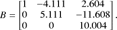$$B=\left[\begin{array}{ccc}1& -4.111& 2.604\\ 0& 5.111& -11.608\\ 0& 0& 10.004\end{array}\right].$$(37)

We tested the method by numerical simulations in which we built a probability distribution for v and r (e.g., Gaussian distributions, see Fig. 15), then we projected these to v_z and r_p and computed the resulting $r_p{v}_z^2$ distribution.Whatever the initial 3D distribution, the projected distribution is strongly decreasing, as expected from the shape of the projection function p_η(η) (see Fig. 4). This property is the reason why it is so difficult to estimate the pair mass (Faber & Gallagher 1979). However, despite this problem, our new method allows us to recover the 3D PDF of rv² with a fair accuracy (see Figs. 15 and 16).

This yields the total mass M of the system for circular orbits, but in the general case, where r and v are instantaneous values on elliptical orbits, there is, as previously specified, an additional uncertainty to go from the rv² distribution to the M distribution, which may be estimated from an evaluation of the eccentricity distribution. This will be studied in a forthcoming work.

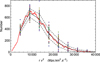Fig. 16 Simulation of 100 random projections of an initial distribution (given by the red curve, see Fig. 15), followed by their respective deprojections (individual points) using a 10 bin deprojection matrix (see text). This simulation allows us to establish the uncertainty of the deprojection method (dashed curves = ± 1σ).

4 Conclusions

In this paper, we developed statistical methods of deprojection of the main physical parameters of pairs of astronomical objects (in particular, galaxy pairs). These methods are needed since, in the extragalactic domain, only one component of the intervelocityand two components of the interdistance are available on only one point of the orbit instead of the six (x_k, v_k) coordinates on the full orbit.

We analytically determined the various PDFs of the projected variables: radial velocity v_z, projected interdistance on the sky-plane r_p, their ratio r_p ∕v_z, which can be used as signature of circular orbits, and $r_p{v}_z^2$, which intervenes in the calculation of the pair mass. These analytical solutions were validated by numerical simulations.

Then we described in detail the deprojection methods obtained by inversion of these projection functions. These methods were conceived in a digitalized way to deal with the real data that will be available in the form of histograms.

In this paper, we prepared the application to effective extragalactic galaxy pair data, and in particular to the two galaxy pair catalogs that we recently constructed, one of which contains 13 000 pairs (Nottale & Chamaraux 2018). These numerical simulations support the validity of our deprojection methods, and they also allow us to determine their error bars.

In a forthcoming work, we will apply these deprojection methods to the study of the physics of galaxy pairs, in particular to their dynamics. Such a study will then benefit from twin improvements to catalogs (membership criteria, data quality, and size) and to methods aiming at statistically recovering missing information.

Appendix A Various probability distributions

A.1 Probability distribution of a product of two variables

Consider two random variables x and y whose probability distribution p(x, y) is known. The probability distribution of the product η = xy is given by Rohatgi (1976) and Glen et al. (2004) $$p_{\eta }(\eta )={\displaystyle {\int }_{-\infty }^{+\infty }{p}_{xy}}\left(x,\frac{\eta }{x}\right)\frac{1}{\left|x\right|}\text{\hspace{0.17em}d}x.$$(A.1)

It becomes in the uncorrelated case, where we have p_xy (x, y) = p_x(x) p_y(y), 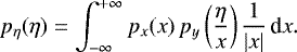$$p_{\eta }(\eta )={\displaystyle {\int }_{-\infty }^{+\infty }{p}_x}(x)p_y\left(\frac{\eta }{x}\right)\frac{1}{\left|x\right|}\text{\hspace{0.17em}d}x.$$(A.2)

A.2 Probability distribution of the inverse of a variable

Let x be a random variable of probability distribution p_x (x). The probability distribution of its inverse X = 1∕x is written as $$p_X(X)=\frac{1}{X^2}{p}_x\left(\frac{1}{X}\right).$$(A.3)

A.3 Probability distribution of the ratio of two variables

From these two relations we easily derive the probability distribution of the ratio of two random variables, ζ = y∕x. We find $$p_{\zeta }(\zeta )={\displaystyle {\int }_{-\infty }^{+\infty }}{p}_{xy}\left(x,\zeta x\right)x\text{\hspace{0.17em}d}x.$$(A.4)

Appendix B Circular orbits

We give here a criterion for identifying circular orbits (and more generally, all configurations when the vectors v and are perpendicular). We consider the scalar product of the position and velocity vectors, i.e., $$x{v}_x+y{v}_y+z{v}_z=rv\cos \varphi ,$$(B.1)

where ϕ is the angle between the two vectors. This relation is written in cylindrical coordinates as $$r_p{v}_p\cos {\varphi }_p+z{v}_z=rv\cos \varphi ,$$(B.2)

where ϕ_p is the angle between the projected vectors v_p and r_p on the plane of the sky. Since $r^2=r_p^2+z^2$ and $v^2=v_p^2+v_z^2$, the ratio of the two observables v_z and r_p is written as 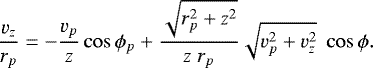$$\frac{v_z}{r_p}=-\frac{v_p}{z}\cos {\varphi }_p+\frac{\sqrt{r_p^2+z^2}}{z{r}_p}\sqrt{v_p^2+v_z^2}\cos \varphi .$$(B.3)

When the velocity vector v is perpendicular to the position vector r, we have cosϕ = 0 and therefore this formula takes the simplified form 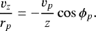$$\frac{v_z}{r_p}=-\frac{v_p}{z}\cos {\varphi }_p.$$(B.4)

The statistical distribution of the ratio v_z∕r_p is therefore expected to be very different between the orthogonal case and the general case, providing us with a statistical signature for circular orbits.

Let us establish the theoretical expectation of this distribution.

In the case when r and v are perpendicular, which corresponds to circular orbits and to special positions on elliptic orbits, the distributions of v_z and r_p become highly correlated. In particular, let us show that, in this case, |v_z |∕v ≤ r_p∕r.

Let us set α = (xv_y)∕(yv_x), we have ${(\alpha -1)}^2\ge 0$, which may be written as α + 1∕α ≥ 2, i.e., $$\frac{1}{2}\left(\frac{x}{y}\frac{v_y}{v_x}+\frac{y}{x}\frac{v_x}{v_y}\right)\ge 1.$$(B.5)

The orthogonality of r and v writes xv_x + yv_y + zv_z = 0, such that $$z^2{v}_z^2={(x{v}_x+y{v}_y)}^2.$$(B.6)

Accounting for this relation, the inequality (B.5) becomes $$v_z^2(x^2+y^2+z^2)\le (x^2+y^2)(v_x^2+v_y^2+v_z^2),$$(B.7)

i.e., |v_z| r ≤ r_p v, QED.

This means that for given r, v and r_p, the possible values of v_z are no more uniform between 0 and v, but are limited to v_z ≤ v r_p∕r.

References

All Figures

Fig. 1 Theoretical expectation vs. numerical simulation of the statistical distribution of vz ∕v, where vz is the radial velocity difference between galaxies in randomly oriented pairs and v the true velocity difference. The number of simulated pairs is here N ≈ 10 000. Apart from statistical fluctuations, the obtained probability distribution of the radial velocity is constant in the range [0, v], in agreement with the theoretical expectation (given by the constant red line).

In the text

Fig. 2 Numerical simulation of the probability density distribution of rp∕r, where rp is the projection on the plane of the sky of the distance r between members of randomly oriented pairs (for a fixed 3D r value). The number of simulated pairs is N ≈ 10 000. Apart from statistical fluctuations, the obtained probability distribution agrees with the theoretical expectation (continuous red line, see text).

In the text

Fig. 3 Numerical simulation of the density distribution of the ratio rp∕vz, where rp is the distance between pair members projected on the plane of the sky and vz is their radial velocity difference (here with r = 1 and v = 1). The number of simulated pairs is N = 4000. Within statistical fluctuations, the obtained probability distribution agrees well with the theoretical expectation (red continuous line, Eqs. (11) and (12)). In the case of circular orbits, the velocity and radial vectors are orthogonal, which implies rp ∕vz ≥ r∕v (see text), i.e., rp∕vz ≥ 1 in this figure. That achieves a clear signature of circular orbits, for which the left part of the figure (rp ∕vz < 1) below the sharp peak of the rp∕vz PDF is expected to be empty.

In the text

Fig. 4 Analytical formula (see text) vs. numerical simulation of the density distribution of the product $r_p{v}_z^2$, where rp is the distance between pair members projected on the plane of the sky and vz is their radial velocity difference. This combination of variable is essential for the statistical determination of the total mass of the pair. The product is plotted here for r = 1 and v = 1, i.e., the plotted variable is actually $(r_p/r){(v_z/v)}^2$. The number of simulated pairs is N ≈ 10 000. Within statistical fluctuations, the obtained probability distribution agrees well with the theoretical expectation (red line, Eq. (20)).

In the text

Fig. 5 Illustration of the deprojection method for radial velocity (or any 1D variable projected from a 3D vector). For a bin (V i−1, V i) of width δV, where V i = i × δV, Ni is the number of values contained in this bin in the histogram of the projected quantity. The number of objects that have a deprojected value v = V i is given by the area of the rectangle of height (Ni − Ni+1) and of extent [0, V i].

In the text

Fig. 6 Numerical simulation of the intervelocity deprojection of a sample of 1200 pairs (left figure) and 13 000 pairs (right figure). The original 3D velocities have a Gaussian distribution of standard deviation σv = 90 km s−1 and peak velocity 190 km s−1 (cutoff on V = 0) [red curve]. We randomly project a random realization of this Gaussian distribution, then deproject it using the constant bin method with a bin of width 30 km s−1 (left figure) and 20 km s−1 (right figure, see text). The blue histogram is the mean result of 100 realizations of such a projection/deprojection and the black lines are the ± 1σ lines.

In the text

Fig. 7 Various realizations of the numerical simulation of the intervelocity deprojection (sample of 13 000 pairs). Left figure: an example of a single realization. The original 3D velocities have a Gaussian distribution of standard deviation σv = 90 km s−1 and peak velocity 190 km s−1 (cutoff on V = 0) [red curve]. We randomly projected a random realization of this Gaussian distribution, then deprojected it using the constant bin method with a bin width 20 km s−1 (see text). The blue broken line is the obtained deprojection, compared with the ± 1σ lines estimated from 100 realizations (see Fig. 6). Right figure: various realizations using differences on non-adjacent bins ($N_{i+1}^p-N_{i-1}^p$), for the same original velocity PDF. We randomly projected random realizations of this Gaussian distribution, then deprojected it using the constant bin method (blue histograms) with a bin width 20 km s−1 (see text). The dashed orange lines show the ± 1σ lines estimated from 100 realizations. The quality of the deprojection is improved by a factor of ≈ 2 with respect to the adjacent bin method.

In the text

	Fig. 8 Histogram of the projected velocities (from an initial Gaussian distribution of mean 150 km s−1 and standard deviation 50 km s−1) on a moving bin wbin shifted by differences between bin positions δv = 1 km s−1.
In the text

Fig. 9 Deprojections by constant moving bins method of several realizations of a sample projected from an initial Gaussian distribution (Nv ≈ 1200 points, Ns = 25 realizations). We show the mean deprojected distribution (black curve) and the ± 1σ limits (green curves) compared with the initial distribution (red curve). In the left figure, the peak position is 150 km s−1 and its standard deviation 50 km s−1. The deprojection shows no bias with such a velocity peak width. In the right figure, the peak position is 150 km s−1 and the standard deviation 20 km s−1. The deprojection shows a bias with such a narrow velocity peak width. The deprojected velocity peak is too low by ≈ 12% and too wide by ≈20%, although the peak position is precisely recovered to within ≈1%.

In the text

Fig. 10 Deprojections by the constant moving bins method of several realizations of a sample projected from an initial Gaussian distribution with peak position 150 km s−1 and standard deviation 50 km s−1 (Nv ≈ 12 000 points, Ns = 25 realizations). We show the mean deprojected distribution (black curve) and the ± 1σ limits (greencurves) compared with the initial distribution (red curve). The quality of the deprojection is clearly improved compared to the 1200 points case, in particular concerning the peak amplitude (Fig. 9).

In the text

Fig. 11 Deprojection by a varying moving bin. The bin width varies between 20 and 40 km s−1 dependingon the slope. The obtained distribution is finally smoothed out by a bin width 20 km s−1. We performed several realizations of a sample projected from an initial two-Gaussian peaks distribution with respective peak positions 70 and 150 km s−1 and standard deviations 15 and 20 km s−1 (Nv ≈ 12 000 points, Ns = 25 realizations). We show the initial distribution as a red continuous curve. Despite the narrowness of the peaks, the quality of the deprojection is very good since the two peaks and the intermediate hollow are clearly identified at their true positions.

In the text

Fig. 12 Illustration of the method of deprojection of rp, for 10 bins and an initial distribution Pr(r) = constant between 0 and r0. We show how the initial unprojected number density in each given bin (this initial density is chosen to be constant = 1) is distributed among the original bin and those at smaller distances (areas contained between the broken lines). The red dashed line is the expected distribution [arccos(rp)] in the limit of vanishing bin width (infinite number of bins). Conversely, one can recover the initial unprojected distribution from the projecteddistribution by inverting such a decomposition (see text). There is just a small bias on the first and last bins.

In the text

	Fig. 13 Example of statistical deprojection of rp for a constantPDF of r. We start froma projected distribution Np = arccos(rp) (inclined blue points) for 20 bins (see text). The deprojected probability distribution is shown as almost horizontal magenta points.
In the text

	Fig. 14 Example of deprojection of rp for a projected distribution Np obtained from a 3D (unprojected) initial Gaussian distribution Nr (black histogram, total 10 000 points) for 10 bins. The deprojected probability distribution (magenta points) is in good agreement with the initial probability distribution.
In the text

	Fig. 15 Example of deprojection (points) of a projected distribution $r_p{v}_z^2$ (decreasing blue curve) obtained from a 3D (unprojected) initial distribution r v2 (red curve), for 10 bins. The initial distribution is built from a Gaussian velocity distribution of mean 200 km s−1 and dispersion 50 km s−1 and a Gaussian distance distribution of mean 0.3 Mpc and dispersion 0.05 Mpc.
In the text

	Fig. 16 Simulation of 100 random projections of an initial distribution (given by the red curve, see Fig. 15), followed by their respective deprojections (individual points) using a 10 bin deprojection matrix (see text). This simulation allows us to establish the uncertainty of the deprojection method (dashed curves = ± 1σ).
In the text

References

- Alam, S., Albareti, F. D., Allende Prieto, C., et al. 2015, ApJS, 219, 12 [NASA ADS] [CrossRef] [Google Scholar]
- Bergstrom, L. 2000, Rep. Prog. Phys, 63, 793 [NASA ADS] [CrossRef] [Google Scholar]
- Chamaraux, P., & Nottale, L. 2016, VizieR Online Data Catalog: J/other/AstBu/71.270 [Google Scholar]
- Chavanis, P. H. 2017a, Eur. Phys. J. Plus, 132, 286 [CrossRef] [Google Scholar]
- Chavanis, P. H. 2017b, ArXiv e-prints [arXiv:1706.05900] [Google Scholar]
- Chengalur, J. N., Salpeter, E.E., & Terzian, Y. 1996, ApJ, 461, 546 [NASA ADS] [CrossRef] [Google Scholar]
- Faber, S. M., & Gallagher, J. S. 1979, ARA&A, 17, 135 [NASA ADS] [CrossRef] [MathSciNet] [Google Scholar]
- Glen, A. G., Leemis, L. M., & Drew, J. H. 2004, Comput. Stat. Data Anal., 44, 451 [CrossRef] [Google Scholar]
- HyperLEDA database 2016, http://leda.univ-lyon1.fr [Google Scholar]
- Makarov, D., Prugniel, P., Terekhova, N., Courtois, H., & Vauglin, I. 2014, A&A, 570, A12 [NASA ADS] [CrossRef] [EDP Sciences] [Google Scholar]
- Nilson, P. N. 1973, Uppsala General Catalogue of Galaxies (UGC), Uppsala Obs. Ann., 6 [Google Scholar]
- Nottale, L., 2011, Scale Relativity and Fractal Space-Time: A New Approach to Unifying Relativity and Quantum Mechanics (London: Imperial College Press), 764 [Google Scholar]
- Nottale, L., & Chamaraux, P. 2018, Astrophys. Bull., submitted [arXiv:1706.06482] [Google Scholar]
- Peterson, S. D. 1979, ApJS, 40, 527 [NASA ADS] [CrossRef] [Google Scholar]
- Rohatgi, V. K. 1976, An Introduction to Probability Theory, Mathematical Statistics (New York: Wiley) [Google Scholar]
- Sanders, R. H., & McGaugh, S. S. 2002, ARA&A, 40, 263 [NASA ADS] [CrossRef] [Google Scholar]