| Issue |
A&A
Volume 614, June 2018
|
|
|---|---|---|
| Article Number | A69 | |
| Number of page(s) | 15 | |
| Section | The Sun | |
| DOI | https://doi.org/10.1051/0004-6361/201732298 | |
| Published online | 14 June 2018 | |
Solar type III radio burst time characteristics at LOFAR frequencies and the implications for electron beam transport
SUPA School of Physics and Astronomy,
University of Glasgow,
Glasgow
G12 8QQ,
UK
e-mail: This email address is being protected from spambots. You need JavaScript enabled to view it.
Received:
15
November
2017
Accepted:
24
January
2018
Abstract
Context. Solar type III radio bursts contain a wealth of information about the dynamics of electron beams in the solar corona and the inner heliosphere; this information is currently unobtainable through other means. However, the motion of different regions of an electron beam (front, middle, and back) have never been systematically analysed before.
Aims. We characterise the type III burst frequency-time evolution using the enhanced resolution of LOFAR (LOw Frequency ARray) in the frequency range 30–70 MHz and use this to probe electron beam dynamics.
Methods. The rise, peak, and decay times with a ~0.2 MHz spectral resolution were defined for a collection of 31 type III bursts. The frequency evolution was used to ascertain the apparent velocities of the front, middle, and back of the type III sources, and the trends were interpreted using theoretical and numerical treatments.
Results. The type III time profile was better approximated by an asymmetric Gaussian profile and not an exponential, as was used previously. Rise and decay times increased with decreasing frequency and showed a strong correlation. Durations were shorter than previously observed. Drift rates from the rise times were faster than from the decay times, corresponding to inferred mean electron beam speeds for the front, middle, and back of 0.2, 0.17, 0.15 c, respectively. Faster beam speeds correlate with shorter type III durations. We also find that the type III frequency bandwidth decreases as frequency decreases.
Conclusions. The different speeds naturally explain the elongation of an electron beam in space as it propagates through the heliosphere. The expansion rate is proportional to the mean speed of the exciter; faster beams expand faster. Beam speeds are attributed to varying ensembles of electron energies at the front, middle, and back of the beam.
Key words: Sun: flares / Sun: radio radiation / Sun: particle emission / solar wind / Sun: corona
e-mail: This email address is being protected from spambots. You need JavaScript enabled to view it.
© ESO 2018
1 Introduction
Type III radio bursts are understood to be signatures of accelerated electrons in the solar corona and interplanetary space. Analysis of their frequency-time profile allows electron beam characteristics to be diagnosed close to the Sun, where spacecraft are unable to make in situ plasma measurements. The rapid change in the frequency of these radio bursts is attributed to the high velocities of the electron beams, which are around 0.3c, where c is the speed of light. The time profiles at an individual frequency provides information about the spatial and energetic profiles of the electrons that participate in the plasma emission mechanism as well as the radio-wave escape from the turbulent solar corona.
The time profile of type III radio bursts has been studied by numerous authors (e.g. Hughes & Harkness 1963; Aubier & Boischot 1972; Evans et al. 1973; Alvarez & Haddock 1973a; Barrow & Achong 1975; Poquerusse 1977; McLean & Labrum 1985; Tsybko 1989; Mel’Nik et al. 2011) to investigate electron beam and background plasma parameters. At a given frequency, it was suggested early on (see Aubier & Boischot 1972, for a complete explanation) that the type III burst could be made up of an exciter function followed by an exponential decay, as there is an observed asymmetry in the type III light curve. It was believed that the exciter envelope was possibly driven by the motion of the electron beam, whilst the damping exponential was driven by a separate process. Consequently, the bulk of the time profile analysis was heavily focussed in this idea, to the detriment of analysing the rise time of the radio burst profile before the peak time.
One initial theory for the damping time, and motivation for an exponential function, was that collisional damping was responsible and so plasma temperatures could be inferred (see Riddle 1974, for a discussion). Temperatures that were similar to coronal temperatures were inferred at high frequencies. However, studies (e.g. Evans et al. 1973; Alvarez & Haddock 1973a; Takakura et al. 1975; Poquerusse et al. 1984; Ratcliffe et al. 2014) found that collisional times cannot correctly explain radio burst decay times correctly, particularly near 1 AU.
Large-scale density inhomogeneity reduces the energy of the beam and must play a key role in establishing the decay profile. As an electron beam exchanges energy with Langmuir waves during propagation, these waves are refracted to lower phase velocities by the large-scale density inhomogeneity in the radially decreasing solar corona and solar wind (e.g. Kontar 2001a). Langmuir waves are absorbed by the background plasma, depleting energy from the beam-plasma system (e.g. Kontar & Reid 2009; Reid & Kontar 2013). Density inhomogeneities can suppress the generation of radio emission in the presence of significant Langmuir wave populations (Ratcliffe & Kontar 2014). The characteristic time for density inhomogeneity tracked the half-width, half-maximum decay time of simulated type III bursts (Ratcliffe et al. 2014). The simulated time profiles were nearly symmetric around the peak time, and so density inhomogeneity might not be the dominant process when the time profile is highly asymmetric.
The scattering of light from source to observer (Steinberg et al. 1971; Riddle 1972) has also been suggested to account for the exponential decay time seen in radio bursts, particularly at lower frequencies where the time profile is increasingly asymmetric.Moreover, the early observations were unable to distinguish intrinsic and radio-wave propagation effects. Recent imaging andspectroscopic observations of the fine structures (Kontar et al. 2017) demonstrated that radio-wave propagation effects, and not the properties of the intrinsic emission source, dominate the observed spatial characteristics and hence play an important role for the time profile.
The characteristic exponential decay time that was found from fits to radio bursts increases as a function of decreasing frequency (e.g. Aubier& Boischot 1972; Evans et al. 1973; Alvarez & Haddock 1973a; Barrow & Achong 1975; Poquerusse 1977). This increase can be fit with a power law over a wide range of frequencies (Alvarez & Haddock 1973a), finding a spectral index close to one. At different frequencies, the decay time has been found to be proportional to the duration of type III bursts, using the full-width at half-maximum of the flux profile. Later, Poquerusse (1977) found the same relation at a single frequency, around 169 MHz, and proposed that both quantities are linked to the electron beam dynamics at this frequency rather than the decay constant being linkedto the ambient plasma, as was previously expected. Whether this result holds true at lower frequencies when the time profile is more asymmetrical has not be researched.
The exciter profile of the type III bursts (rise above background until part way through the decay phase) follows the same trend, increasing as a function of decreasing frequency (e.g. Aubier & Boischot 1972; Evans et al. 1973; Barrow & Achong 1975). The study by (Evans et al. 1973) fit a linear relation as a function of decreasing frequency between 2.8–0.067 MHz. The exciter times do not analyse the rise time, that is, the rate of increase before the peak flux, of the type III bursts. This has not been adequately researched in the literature. Poquerusse (1977) approximated the rise time at 169 MHz using the slope of the linear rise, finding it to scale with the slope of the decay, although with asymmetry.
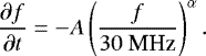
The drift rate  (measured in MHz s−1) is typically found using the peak time in each frequency channel. A study by Alvarez & Haddock (1973b) collated numerous observations to plot the change in drift rate as a function of frequency, finding a power law over four orders of magnitude between 1000–0.1 MHz, such that
  , where f is measured in MHz and t is measured in seconds. Since then, studies (e.g. Achong & Barrow 1975; Mel’Nik et al. 2011) have found drift rates that are slightly lower than predicted by Alvarez & Haddock (1973b) at frequencies above 10 MHz.
The velocity of electron beams is typically deduced using the drift rate and assumptions regarding the background density model and emission mechanism. Typical velocities are around 0.3 c but can have a broad range from 0.1–0.5c (Suzuki & Dulk 1985; Reid & Ratcliffe 2014; Carley et al. 2016). Whilst not being mono-energetic, single velocities are usually derived from radio bursts. Electrons over a range of velocities are believed to collectively move in a beam-plasma structure (e.g. Ryutov & Sagdeev 1970; Kontar et al. 1998; Mel’Nik et al. 1999) at the average velocity of the participating electrons. The velocity of electron beams as derived from type III bursts has been reported to be slowing down as the beams propagate through the heliosphere (Fainberg et al. 1972; Krupar et al. 2015; Reiner & MacDowall 2015). The drift rate has been investigated using the onset time rather than the peak time observationally (Fainberg et al. 1972; Dulk et al. 1987; Reiner & MacDowall 2015) and numerically (Li & Cairns 2013), and a faster velocity was obtained, postulating that the front of the electron beam travels with a faster velocity. Derived electron beam velocities are also dependent upon the conditions of the background plasma, with Li & Cairns (2014) showing that a background Kappa distribution resulted in faster derived velocities than when the background had a Maxwellian distribution.
The bandwidth of the type III bursts (the instantaneous width in frequency space) has rarely been analysed. A broad instrumental coverage in frequency space is required to ascertain the spectral width. The coherent plasma emission mechanism causes the intensity of radio emission to increase as a function of decreasing frequency down to 1 MHz (e.g. Dulk et al. 1998; Krupar et al. 2014). The spectral extent of the radio burst therefore needs to be defined carefully. The bandwidth of type III bursts typically decreases as a function of decreasing frequency. An early study by Hughes & Harkness (1963) found a bandwidth of 100 MHz with a minimum frequency of 100 MHz, although they did not state exactly how the minimum and maximum frequencies were defined from the light curve. Mel’Nik et al. (2011) reported a bandwidth from 20 MHz with frequency 27 MHz down to 10 MHz at frequency 12 MHz, although again they did not state how they defined the bandwidth. Mel’Nik et al. (2011) also provided the relation Δ f = 0.6fpe, where  for the bandwidth, assuming fundamental emission at fpe for a background electron density ne.
In this work, we analyse type III profiles and find rise, peak, and decay times between 70–30 MHz. The LOFAR observations allow estimates for these quantities with a high degree of accuracy. After explaining how we use the observations in Sect. 2, we present the temporal observations in Sect. 3. In Sect. 4 we show how these quantities drift through time and frequency and use the results to discuss the electron beam parameters in Sect. 5. We explain how the electrons move through space in Sect. 6, and conclude with our results in Sect. 7.
2 Observations
2.1 Event list
We used a selection of type III bursts observed by LOFAR (van Haarlem et al. 2013) between April–Sept 2015. LOFAR was only observing for two-hour intervals on specific days. As our goal was to characterise the behaviour of individual events, we only selected isolated type III bursts. We thus ignored type III bursts that overlapped with other radio activity, showed too much fine structure, or were too faint to be detected between frequencies 70–30 MHz. We selected 31 type III bursts that satisfied these criteria.
The LOFAR observations were taken using a time resolution of about 0.01 s. To improve the signal-to-noise ratio, the observations were integrated to a time resolution of about 0.1 s. The frequency range around 80–30 MHz was covered by 258 sub-bands, each with 16 channels. Again, to improve the signal-to-noise ratio, we integrated over each channel to use the 0.195 MHz sub-band frequency resolution. The sub-band frequency resolution is comparable to the frequency resolution of similar instruments (e.g. the Nançay Decametre Array), but the enhanced signal-to-noise ratio resolution provides light curves with a small standard deviation for an accurate fitting analysis. The dynamic spectra were taken as an average over 169 dynamic spectra using the LOFAR tied-array mode (Stappers et al. 2011), pointed at different positions across the solar disc (e.g. Morosan et al. 2014; Reid & Kontar 2017a). Whilst we used measurements between 80–30 MHz to obtain our results, the number of radio bursts with a high signal-to-noise ratio above 70 MHz was small. We therefore only report the trends in characteristic times between 70–30 MHz.
2.2 TypeIII flux profile
Type III flux profiles as a function of time and frequency provide information on the dynamics of electron beams that propagate through the solar corona and the heliosphere. In this study, we are particularly interested in the rise, peak, and decay times at individual frequencies, together with the variation of these parameters as a function of frequency.
Whilst obtaining these parameters directly from the data measurements is desirable, accuracy in time is restricted to the cadence of the measurements, and fluctuations in the data from noise can cause spurious results. Moreover, the background flux must be accounted for. To resolve these problems, we fit the flux as a function of time and obtained characteristic parameters from the fit.
Previous studies (e.g. Aubier & Boischot 1972; Evans et al. 1973; Achong & Barrow 1975) have not characterised a rise or decay profiles, but assumed an exponential decay function (see e.g. Aubier & Boischot 1972; Evans et al. 1973, for an example). We make nosuch assumptions and use the half-width, half-maximum (HWHM) to characterise rise and decay. Whilst the exponential function is a reasonable approximation for the decay constant, it is not a good envelope for the entire flux profile. The peak of the type III burst time profile with a high temporal resolution typically has a rounded top that is inconsistent with exponential decay.
To assess whether an exponential or Gaussian function best characterises the type III flux profile, we first subtracted a background B(f) from the type III flux profiles. We found the background for each frequency sub-band by taking the mean flux over a period of 3–5 min when there was reduced activity during the observations. The background B(f) is assumed to be constant in time. The LOFAR observations of type III burst time profile (Kontar et al. 2017) suggest an asymmetric time profile at 30–40 MHz. Therefore, we fit the intensity of the type III bursts for each frequency using an exponential function of the asymmetric form
 (1)
(1)
A different characteristic rise and decay is required to capture the asymmetry in the type III flux around the peak time. We also fit the type III bursts using a Gaussian function of the form
 (2)
(2)
All fitting in this work was done using mpfitfun and mpfitexy (Markwardt 2009), which provides an associated statistical error on each fitting parameter.
An example flux profile is shown in Fig. 1 along with a Gaussian and exponential fit to the data. The rise and decay times,tr and td, were characterised using the half-width, half-maximum from each fit (e.g. for the rise time, exponential tr = τr log(2), and Gaussian  ). We also found the HWHM directly from the data using the point farthest from the peak with a flux of at least 50% of the peak flux. A comparison found that the Gaussian fit was substantially closer to the HWHM found from the data. The exponential function typically underestimated the rise and decay times, as shown in Fig. 1. The decay time from the exponential fit for a few radio bursts better agreed with the HWHM found from the data. These bursts typically had a larger asymmetry, with the decay times being notably longer than the rise times. However, for consistency, we used a Gaussian fit for all the radio burst time profiles.
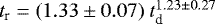
Characterising the rise, peak, and decay times allows us to see how each characteristic time drifts as a function of frequency. Figure 1 shows that these times result in three different drift rates for a single type III burst. The duration tD, found from the FWHM, is also indicated around 48 MHz.
The instantaneous bandwidth of the type III radio burst, that is, the width of the type III burst in frequency space, can be found at each point in time. There is no standard definition as to how the instantaneous bandwidth is found in the literature. We introduce here a technique to define the bandwidth using the type III rise and decay times. At each point in time, we find the highest type III frequency by finding the highest frequency that has not stopped emitting using t0 + td. Similarly, we find the lowest type III frequency by finding the lowest frequency that has started emitting using t0 − tr. The bandwidth is defined as the difference between the highest and lowest frequency.
For the results in this study, we therefore use the Gaussian fit described by Eq. (2) to obtain the parameters of interest for the dynamic spectrum. The following type III parameters are found from the fits:
-
The rise time tr is found at t < t0 from HWHM,
 .
. -
The decay time td is found at t > t0 from the HWHM
 .
. -
The duration tD is found using the full-width half-maximum (FWHM).
-
The drift rate is found from the change in rise, peak, and decay time as a function of frequency.
-
The bandwidth is found from the frequency width between the HWHM at different frequencies.
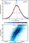 |
Fig. 1 Top: background-subtracted type III flux profile around 48 MHz. The peak flux and HWHM points are shown as green circles. A Gaussian (red) and exponential (blue) fit are shown, together with their peak flux and HWHM. The Gaussian fit tracks the HWHM points in the data better, and the rise, peak, and decay times derived from the Gaussian fit are shown using the red dashed lines. Bottom: dynamic spectrum of the same burst. The drift of the rise, peak, and decay as a function of frequency are shown, together with the duration and bandwidth of the radio burst around 48 MHz. |
3 Type III rise, decay, and duration
3.1 Rise time
The rise time, tr, of the type III bursts for each frequency is determined from the HWHM of the flux before t0, the time of peak flux. Figure 2 shows how the mean rise time varies as a function of frequency over all the type III bursts. The mean is calculated from a weighted function of each radio burst such that
 (3)
(3)
where  is the variance associated with tr,i, obtained from fitting the type III burst profile using mpfit, and the weighted function is
  .
.
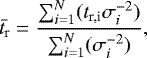
The mean rise time increases as a function of decreasing frequency. We have fitted the change in rise time using a power-law function such that
 (4)
(4)
The error on the rise time for each individual burst is very small, but there is a significant spread in the rise times over all radio bursts, indicated by the standard deviation in the rise times in Fig. 2. Consequently, we used the standard deviation of the frequency and rise times as an error for the fit to account for this wide range in rise times.
Whilst the mean rise time increases as a function of decreasing frequency, the rise time does not increase in such a smooth manner for individual type III bursts. The bursty nature in the dynamic spectrum of type IIIs causes the rise time in some frequency ranges to have constant rise times or steeply increasing rise times, or even decreasing rise times.
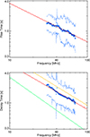 |
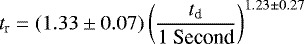
Fig. 2 Mean rise time (top) and decay time (bottom) as a function of frequency for all the analysed type III bursts as found from the HWHM, tr and td, respectively. The top and bottom blue dashed lines show the spread of the data, found from the standard deviation. The red dashed line show the fits tr = (1.5± 0.1) f−0.77±0.14 and td = (2.2 ± 0.2) f−0.89±0.15 for frequency (per 30 MHz). For the decay time, the green and orange dashed lines show the fits from Evans et al. (1973) and Alvarez & Haddock (1973a), respectively, assuming a HWHM of td = τd log(2), from the derived exponential profiles τd. |
3.2 Decay time
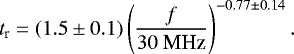
The decay time, td, for each frequency is determined from the HWHM of the flux after t0, the time of peakflux. Figure 2 shows the variation in the mean decay time as a function of frequency over all type III radio bursts. The mean is calculated from a weighted function of each radio burst using Eq. (3) with td,i instead of tr,i. The spread in the decay times is indicated by the standard deviation in the decay times in Fig. 2.
We have fitted the decay time using a power-law function such that
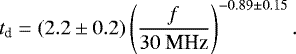 (5)
(5)
We used the standard deviation of the frequency and decay time as an error for the fit. The spectral index b captures the general trend that the decay time increases as a function of decreasing frequency. The decay times are slightly shorter than the decay times found from numerical simulations of a type III burst (Ratcliffe et al. 2014), which had a decay of 1 s around 100 MHz and 8 s around 10 MHz.
We can compare our results to the previous fit found from Alvarez & Haddock (1973a), who used an exponential function to obtain a characteristic decay constant τd. They fit data from multiple studies between the frequencies 0.06–200 MHz (only two data points below 0.2 MHz), finding τd = 4f−0.95 for the frequency f (per 30 MHz). We scaled τd to the HWHM using td = τd log(2). The corresponding fit is over-plotted in Fig. 2. The slope agrees well with our observations, being within one standard deviation, but the absolute magnitude is higher.
The characteristic decay constant τd for type III bursts was also analysed by Evans et al. (1973), but between the frequencies 2.8–0.067 MHz. They used a similar exponential fit, finding  for the frequency f (per 30 MHz). Again, we scaled τd to the HWHM using td = τd log(2). Over-plotting the fit on Fig. 2 shows that extrapolating the fit from lower frequencies back to higher frequencies does not obtain an accurate prediction. The comparison suggests that a single power-law might not capture the increase in the decay rate as a function of decreasing frequency from the corona (e.g. 50 MHz) all the way out into interplanetary space (e.g. 50 kHz).
3.3 Asymmetry in the time profile
Type III time profiles typically show asymmetry, with the decay time being longer than the rise time. Figure 3 shows the rise time plotted against the decay time along with the associated errors from the fitting. The asymmetry is clear, with the decay time being longer than the rise time in 77% of the time profiles. The Pearson correlation coefficient is 0.51 and does not change much when considering the asymmetry of the rise and decay time at individual frequencies.
A correlation has been shown between the mean duration and the mean decay constant for type III bursts as a function of frequency (e.g. Aubier & Boischot 1972; Barrow & Achong 1975; Poquerusse 1977; Abrami et al. 1990). In a similar vein, Fig. 3 shows that the mean rise time and mean decay time are correlated, with a Pearson correlation coefficient of 0.95. We have fitted the ratio using a power-law function such that
 (6)
(6)
using the standard deviation of both variables as an error for the fit. Figure 3 also shows the general trend of an increase in the ratio of decay time over rise time as the frequency decreases.
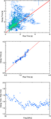 |
Fig. 3 Top: asymmetry of the type III burst time profile along with the errors (in blue) on the rise and decay times. The red line highlights y = x. It is clear that the decay times are longer than rise times, with 77% of the time profiles having a longer decay time than rise time. Middle: mean rise time vs mean decay time, including the power-law fit to the data |
3.4 Duration
We classify the type III duration, tD, as the full-width, half-maximum (FWHM) of the type III bursts. Figure 4 shows the variation in the duration as a function of frequency over all the type III bursts, including the corresponding standard deviations. We have fitted the duration using a power-law function such that
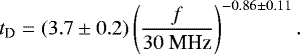 (7)
(7)
The standard deviation of frequency and duration have been used to calculate the errors. The power-law fit shows the general trend of an increasing duration as a function of decreasing frequency.
To compare with other observations, we over-plotted the FWHM as derived by Aubier & Boischot (1972); Barrow & Achong (1975); Tsybko (1989); Mel’Nik et al. (2011) at similar frequencies. We also show the fits for duration as a function of frequency (per 30 MHz) of tD =7.3f−1, reported by Suzuki & Dulk (1985) and tD = 6.2f−2∕3, reported by Elgaroy & Lyngstad (1972). However, we note that the lower-frequency durations involved in the fit by Elgaroy & Lyngstad (1972) were taken from Alexander et al. (1969), who calculated decay times, not durations.The fit therefore underestimates the duration at the low frequencies, which might explain the smaller exponent.
We find that the previously reported mean durations are noticeably higher. Nevertheless, the standard deviations show a wide spread in the duration of the different type III bursts, with past observations being within one standard deviation from our observational mean. Again, the large standard deviations in the duration highlight the spread in values over all the type III radio bursts. The duration of type III bursts must be dependent upon the properties of the electron beams that generated the radio bursts, and perhaps the background plasma properties. This is discussed in detail in Sect. 6.
4 Type III bandwidth and frequency drift
4.1 Bandwidth
The instantaneous bandwidth of a type III radio burst, that is, the width of the type III burst in frequency space, can be found when the highest and lowest frequencies are observed in the dynamic spectrum. As explained in Sect. 2, the bandwidth is defined by the frequency difference between the highest frequency that has not stopped emitting (using t0 + td) and the lowest frequency that has started emitting (using t0 − tr). For each time t, if there are no frequencies where either t0 − td or t0 + tr can be found from the dynamic spectrum, then the bandwidth is not defined.
Figure 5 shows the variation in the bandwidth as a function of frequency for all the type III bursts. The bandwidths are lower than what has been reported by Hughes & Harkness (1963); Mel’Nik et al. (2011). However, this is likely related to their definition of the bandwidth: Hughes & Harkness (1963) used the minimum frequency to report the bandwidth, whilst we used the central frequency.
From numerical simulations, Ratcliffe et al. (2014) reported the bandwidth of a type III burst, also finding slightly higher bandwidths, with a relation of Δf = 0.57f at frequencies 20–100 MHz, slightly decreasing at lower frequencies. Again, the bandwidth was found in a slightly different way, using the FWHM in frequency space. We refrained from using this method as it will be affected by the reported type III burst tendency for the radio flux to increase with decreasing frequencies until 1 MHz (e.g. Krupar et al. 2014), creating a skewed distribution. Ratcliffe et al. (2014) fit the ratio Δ f∕f and found a roughly constant value of Δf∕f = 0.57 above 30 MHz. We found a slightly lower relation of Δf∕f = 0.44 − 0.0017f for the frequency (per MHz). However, the scatter on our bandwidth measurements is quite significant, and the small, frequency-dependent component is likely related to the reduced observations around 65 MHz.
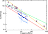 |
Fig. 4 Mean duration as a function of frequency for all the type III bursts, as found from the FWHM. The blue dashed lines show the spread in the data from the standard deviation. The red dashed line shows the fit tD = (3.7 ± 0.2) f−0.86±0.11 for the frequency (per 30 MHz). The purple diamonds show the FWHM found from Aubier & Boischot (1972) and Barrow & Achong (1975). The purple pluses and triangles show the FWHM for fundamental and harmonic bursts, respectively, from Tsybko (1989). The purple squares show the FWHM for powerful (> 1000 SFU) type III bursts, from Mel’Nik et al. (2011). The orange and green dashed lines show the fit in frequency (per 30 MHz) of tD = 7.3f−1 reported by Suzuki & Dulk (1985) and tD = 6.2f−2∕3 reported by Elgaroy & Lyngstad (1972), respectively. |
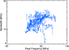 |
Fig. 5 Bandwidth Δf of the type III bursts as a function of peak frequency. |
4.2 Drift rate
The type III frequency drift rate  is typically measured using the peak of the radio time profile. Characterising the time profile of the type III bursts allows us to find the drift rate not only for the peak time of each radio burst, but also for the rise time and the decay time using the HWHM. The drift rate is known to vary as a function of frequency (Alvarez & Haddock 1973b). The increased spectroscopic resolution of LOFAR allows the drift rate to be approximated in small bands. We assumed a constant drift rate over a frequency width of 3 MHz (15 sub-bands). The drift rate over each 3 MHz band was then calculated from a straight line fit
  , together with the one-sigma error on the fit.
Figure 6 shows the change in the drift rate as a function of frequency, where the frequency is found from the central frequency from the 15 sub-bands, and the error on the fit is the corresponding standard deviation. A power-law fit to the data is shown using
 (8)
(8)
The fit obtained from Alvarez & Haddock (1973b) from the frequency (per 30 MHz) is 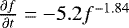 and is shown for comparison in Fig. 6. The drift rates for the rise, peak, and decay times all have a noticeably lower magnitude than those observed by Alvarez & Haddock (1973b). These lower magnitudes agrees with the type III drift rates found by Achong & Barrow (1975) between 18–36 MHz and the drift rates found by Mel’Nik et al. (2011) between 10–30 MHz for powerful (> 1000 SFU) type III bursts.
The drift rates associated with the rise times are marginally higher than those of the peak and higher still than the decay times. The spectral index is slightly lower for all three times, but is within at least two standard deviations of the slope found by Alvarez & Haddock (1973b).
The drift rates from the peak times are very similar to the drift rates obtained from peak times in the numerical simulations by Ratcliffe et al. (2014), with the power-law fit having almost identical parameters. The spread in the observed drift rates is too large to make any meaningful conclusions about whether multiple power-laws over different frequency ranges, used by Ratcliffe et al. (2014), would be a better fit than a single power-law fit. The drift rates are also similar to simulated type III bursts at 85 MHz and >100 MHz by Li et al. (2008); Li & Cairns (2013).
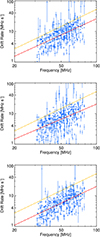 |
Fig. 6 Drift rate as a function of frequency for all type III bursts for the rise (top), peak (middle), and decay (bottom) times. The red dashed line shows the fitted power-law to the data. The orange dashed line shows the fit from (Alvarez & Haddock 1973b). The reduced one-sigma errors are obtained from the fitting uncertainties in the drift rate, taking into account the fitting uncertainties in t0. |
4.3 Drift rate and duration
The duration and drift rates of type III bursts are calculated from different aspects of the dynamic spectrum. It is not immediatelyobvious that they would be related, other than their dependence on frequency. The drift rate decreases as a function of frequency, as shown in Fig. 6. Similarly, the duration increases as a function of frequency, as shown in Fig. 4. We can therefore assume that the drift rate will decrease as the duration increases.
By characterising each individual type III bursts over the entire spectral range of 70–30 MHz, we can remove the frequency dependence.Figure 7 compares the mean duration with the mean drift rate found from the gradient of a linear fit to frequencywith time. The trend is that radio bursts with faster drift rates have a shorter duration. The correlation coefficient is 0.73.
5 Electron beam velocities
5.1 Beam velocities
To explain the temporal behaviour of the type III emission as a function of frequency, we must consider the dynamics of the electron beam exciter and how it interacts with the background electron density to produce the Langmuir waves that are ultimately responsible for the observed radio waves. The type III drift rate is related to the background electron density gradient  and the electron beam velocity
  such that
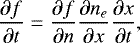 (9)
(9)
where x is the radial propagation distance and ne is the background electron density that produces the radio frequency f. Equation (9) shows that to obtain frequency drift rates with a smaller magnitude than (Alvarez & Haddock 1973b), we are observing either beams with lower velocities or flux tubes with shallower density gradients.
We can estimate the beam velocities with a straight line fit to distance and time using Eq. (9) if we assume the Parker (1958) density model using a normalisation coefficient given by Mann et al. (1999) and second-harmonic emission. The same density profile for all radio bursts introduces a non-statistical error into any beam velocities; the background density gradient probably does not change on timescales comparable to the electron beam velocity, but will be different from burst to burst. The peak time t0 will provide an estimate of the velocity at the middle of the electron beam. The leading edge of the electron beam will cause the generation of the first radio waves in time. Consequently, a velocity for the front of the electron beam can be found using the peak time minus the rise time, t0 − tr. Similarly, a velocity for the back of the beam can be found from the peak time plus the decay time, t0 + td.
We calculated the velocities of the electron beams from the rise, peak, and decay times. Figure 8 shows the velocities for each type III burst using the Parker model. The mean and standard deviation for the velocities are shown in Table 2. The common trend is that the rise velocity is faster than the peak velocity, which in turn is faster than the decay velocity. This is expected behaviour as the bump-in-tail instability that drives the production of Langmuir waves is caused by faster electrons that outpace the slower electrons. The rise time depends upon the length of interval between the front and middle of the electron beam producing a significant radio emission at a certain frequency. If the rise time increases as a function of decreasing frequency, this time period increases with radial distance from the Sun. The velocity of the front of the electron beam will therefore be faster than the velocity of the middle of the electron beam. A similar effect occurs between the middle and back of the electron beam.
Our velocity calculations assumed a 1–1 relation between the intensity of Langmuir waves and the intensity of radio emission. Numerical simulations of type III bursts from an initial Maxwellian beam (e.g. Li et al. 2011) and power-law electron beams (Li et al. 2011; Ratcliffe et al. 2014) show close similarities between the speed of theelectrons and the inferred speed of the exciter from synthetic radio emission. Langmuir waves L excited by faster electrons at the front of the beam are attributed to the onset of fundamental radio emission in (Li & Cairns 2013) due to the process L → T + S for transverse waves T and ion-sound waves S. However, there are differences. For example, the production of second-harmonic emission is intrinsically linked to the number of back-scattered Langmuir waves L′ that are able to take part in the L + L′→ T process (Ratcliffe et al. 2014). Back-scattered Langmuir waves can be produced via Langmuir wave decay, involving ion-sound waves by the processes L + S → L′ and L → L′ + S.
The velocity calculations assume that scattering effects of the radio emission from source to observer do not significantly influence the rise time or the decay time. When scattering is important, scattering is likely to broaden the time profile (Steinberg et al. 1971), decreasing the measured drift rate of type III bursts and slowing down any inferred velocities. The effect on the rise and decay drift rates might be different; quantifying these effects is beyond the scope of this work.
The decay time could also be related to Langmuir waves not being re-absorbed by the electron beam and lingering in space after the beam has moved on. In this case, the background density inhomogeneity will be the primary process in determining the exponential decay rate (e.g. Ratcliffe et al. 2014).
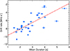 |
Fig. 7 Drift rate as a function of duration for each type III burst. The red dashed line shows the linear fit to the data. |
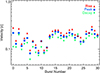 |
Fig. 8 Velocities derived from the rise, peak, and decay times of each type III burst assuming a constant velocity and the Parker density model. For almost all the bursts, the rise time is faster than the peak velocity, which in turn is faster than the decay velocity. The errors on the velocities from the fit are smaller than the symbols. |
5.2 Velocity and duration
The velocityof the type III burst is directly related to the average drift rate. Given the observational correlation between drift rate and duration in Fig. 7, we show the peak velocity as a function of the duration for each type III burst in Fig. 9. The two variables are correlated with a coefficient of 0.73, giving the appearance that a faster electron beam creates radio emission with a shorter duration. The correlation is preserved if we use the front or back velocities, with the latter having a slightly higher correlation coefficient.
The simplest explanation for this correlation is that when the type III duration is shorter, higher-energy electrons are driving the radio emission within the FWHM of the type III burst. The corresponding duration that the electrons spend at any one point in space will therefore be shorter. We discuss the type III duration and electron beam transport in more depth in Sect. 6.3.
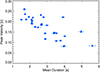 |
Fig. 9 Peak velocities as a function of durations for each type III burst. |
5.3 Beam length velocities
If the front of the electron beam travels faster than the back of the electron beam, then the electron beam will eventually be stretched radially in space to cover a greater length. The difference in electron beam velocity derived from the rise and decay times, Δ v = vr − vd, drives this elongation such that the beam expands at a rate tΔv. This assumes that all velocities are constant in time.
In Fig. 10 we have plotted the length velocity Δ v against the velocity found from the peak. We observe a linear correlation such that faster electron beams have a wider spread between the front and back velocities. The data point in Fig. 10 with a high length velocity is caused by a bright type III burst that had very long decay times between 35–45 MHz. This caused the resulting decay velocity to be anomalously low, and consequently, the length velocity was particularly high. The Pearson correlation coefficient is 0.62 or 0.72, excluding the burst with anomalously high length velocity.
The origin of the correlation is related to the beam-plasma structure (e.g. Mel’Nik & Kontar 1998) that is formed by a propagating electron beam. If the peak velocity is faster, then higher energy electrons are involved in wave-particle interactions with the Langmuir waves that move faster through the background plasma. Consequently, faster velocities of electrons will be involved in the wave-particle interactions at the front of the electron beam. However, the velocity at the back of the electron beam is more dependent upon the background thermal velocity, where Landau damping will ultimately absorb the Langmuir waves with low phase velocities. The difference between the front and back velocities would therefore be larger for beams with higher peak velocities.
The length of the electron beam is directly related to the frequency bandwidth. This means that the change in frequency bandwidth as a function of peak frequency is connected to the length velocity. We can represent the frequency bandwidth using Δ f = fr − fd, where fr, fp, fd are the rise, peak, and decay frequencies at any point in time. The ratio of the bandwidth drift to the frequency drift is then
 (10)
(10)
Using Eq. (9) for the drift rate, we can expand the ratio of bandwidth drift to drift rate to be
 (11)
(11)
If we consider the bandwidth over a time range Δt = t1 − t0 that is sufficiently long, then the range of frequencies for the rise, peak, and decay will be similar. That is, fr (t0) → fr(t1) ≈ fd(t0) → fd(t1). In this case, we can assume that the density gradients ∂nr∕∂xr, ∂np ∕∂xp, and ∂nd ∕∂xd are the same and that the derivatives ∂fr∕∂nr, ∂fp ∕∂np, and ∂fd ∕∂nd are the same. If we assume that the velocities v = ∂x∕∂t are constant, then the ratio of the bandwidth drift to the frequency drift can be expressed as
 (12)
(12)
The ratio of the bandwidth drift to the peak frequency drift is therefore equivalent to the ratio of the length velocity to the peak velocity, independent of the density gradient.
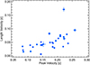 |
Fig. 10 Length velocity (rate at which the electron beam length increases) against the peak velocity. The beam length velocity is derived from the difference between the velocities found from the rise and decay times. |
5.4 Non-constant velocities
In all the above analysis, we assumed that the electron beam velocity remains constant over a finite propagation distance. Deceleration of the exciter has been inferred from the frequency and time of type III observations below 1 MHz (e.g. Fainberg et al. 1972), suggesting a deceleration of 12.3 ± 0.8 km s−2 (Krupar et al. 2015).
To investigate whether a general trend for electron beam deceleration derived from higher frequencies existed, we determined the velocity associated with the drift rate for each 3 MHz interval in a similar way as we obtained the drift rate over the frequency range 70–30 MHz. Figure 11 shows the velocity associated with the drift rates for all the type III radio bursts usingthe Parker (1958) density model and assuming second-harmonic emission. A linear fit to the log of the peak velocities is such that
 (13)
(13)
The change in velocity as a function of distance is very small, with the error on the gradient being significantly higher than the gradient itself. The data therefore does not indicate a strong increase or decrease in the velocity of the electron beam as a function of distance.
A derived velocity is heavily dependent on the density model that is chosen. Taking heights that were derived from observations by Dulk & Suzuki (1980) at 80 and 43 MHz of 0.6 R⊙ and 1.2 R⊙, respectively, we can construct a density model using the assumption that the density decreases exponentially with altitude. The Dulk density model has a smaller density gradient than the model by Parker (1958). Consequently, the derived velocities are higher than those found previously. The mean velocities of the type III bursts shown in Table 2 are approximately 0.08 c faster using the Dulk model, with similar standard deviations.
The second set of derived velocities is shown in Fig. 11 using the Dulk density model. A linear fit to all the velocities shows a trend for the velocity of the exciter to decrease as a function of distance from the Sun. Given the significant differences between the two different models, imaging spectroscopy is likely required to answer this question, taking into account the scattering effects of light from source to observer. The analysis of fine frequency structures suggests significant size increases and a radial shift in position (Kontar et al. 2017).
Velocities for the front, middle, and back of the electron beams using the Parker density model.
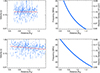 |
Fig. 11 Left: velocities as a function of distance from the Sun for all the type III bursts using the Parker model (top) and the Dulk altitudes (bottom) after t = 5 s. The red line is a linear fit to the log of the velocity such that log10 (v) = ar + c. Right: Frequency and density profiles as a function of altitude for the Parker model (top) and Dulk model (bottom). |
6 Electron beam transport
We have shown that the type III radio data can be used to estimate the velocities associated with the front, middle, and back of the electron beam. However, electron beams are not made up of mono-energetic electrons, but are an ensemble of electrons spread over a range of energies. Why can their travel be approximated by a single velocity, and what exactly dictates how fast they travel? How does this relate to the duration of the electron beam as a function of frequency?
6.1 Gaussian beam
We considerthe transport of a electron beam with a Gaussian distribution in velocity with mean velocity v0 and characteristic velocity Δ v, and a Gaussian profile in space with characteristic length d. The initial electron distribution function is
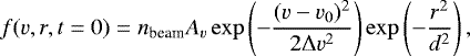 (14)
(14)
where  . The mean velocity v0 = 1010 cm s−1 corresponding to an energy of 28 keV, the density nbeam = 10 cm−3, the width Δv = 109 cm s−1, and the width d = 109 cm. For the Langmuir wave generation, we present two limiting cases. The first limiting case is the free-streaming approximation when the electrons propagate scatter-free. The second is the gas-dynamic theory where the electrons fully interact with waves, propagating in a beam-plasma structure (e.g. Ryutov & Sagdeev 1970; Kontar et al. 1998; Kontar & Mel’Nik 2003). We also present a third case using simulations that lies between these other two.
We consider only particle transport and the quasilinear interaction of particles and waves (Vedenov 1963),
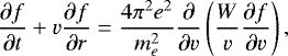 (15)
(15)
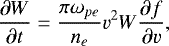 (16)
(16)
where the characteristic propagation time is τp = r∕v and the characteristic quasilinear time is τql = ne∕(πωpenbeam). The background electron density profile has the Parker density profile, as in (Kontar 2001a; Reid & Kontar 2010).
The first limiting case is when the electrons propagate without interacting with Langmuir waves. This case essentially propagates with τql = ∞, so that no waves are generated. Figure 12 shows the distribution function after 5 s. The differences in velocity have elongated the electron beam in space.
The second limiting case is the gas-dynamic theory (GDT; Mel’Nik 1995) that analytically describes the motion of a spatially limited electron beam propagating in a background plasma. The GDT assumes that the quasilinear time τql = 0. A description of the evolution in space of a Gaussian beam is given in Kontar et al. (1998) for electrons with velocity v < v0. A plateau is produced with height nbeam∕v0. The distribution moves with a constant velocity of (v0 + vmin)∕2. A plateau in the electron distribution function is formed in velocity space at every point in position space. The particles and waves propagate together in a beam-plasma structure at a constant velocity determined by the mean velocity in the plateau. The structure can propagate over large distances as it conserves its spatial shape, energy, and the number of particles. Figure 12 shows the distribution function after 5 s for velocities v < v0. There is no spread of the electron beam over distance as the collective motion of the electrons propagate at a single velocity.
The third case is a simulation of the electron beam that evolves using Eqs. (15) and (16). Figure 12 shows the distribution after 5 s. This simulation lies between the two limiting cases. The highest velocities have mostly propagated scatter-free. The lower velocities have formed a plateau and have generated Langmuir waves. Elongation in space of the plateau occurs because the free-streaming electrons become more unstable to Langmuir waves during propagation. The value of τql varies in phase space and also depends upon a number of constants in the initial condition, including nbeam, v0, and Δ v. As an example, as nbeam → 0, the system will propagate as the free-streaming case. As nbeam →∞, the system will propagate in the gas-dynamic case.
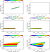 |
Fig. 12 Electron flux (left) and normalised spectral energy density (right) from an initial Gaussian electron beam with v0 = 1010cm s−1 (0.33 c). Top: free-streaming case with zero waves generated. Middle: gas-dynamic theory with electron beam velocities v < v0. Bottom: simulations using Eqs. (15), and (16). |
6.2 Power-law beam
The signature of energetic electrons in the solar atmosphere deduced from X-rays infers a power-law injection function in velocity space (Holman et al. 2011). A complimentary power-law spectrum is measured in situ near Earth (Krucker et al. 2007). We therefore modeled the injection of an electron beam with a power-law distribution in velocity space into a spatially limited acceleration region with a Gaussian profile. The injection function can be described as
 (17)
(17)
where  normalises the injection profile such that the number density injected at r = 0 (acceleration region) is nbeam [cm−3]. The velocity distribution is characterised by α, the spectral index, and the spatial distribution is characterised by d [cm].
Using flare parameters of α = 8, nbeam = 106 cm−3, d = 109 cm, vmin = 2.4 × 109 cm s−1, and vmax = 2 × 1010 cm s−1, we have plotted a snapshot of the electron flux in Fig. 13 at time t = 5 s after free-streaming propagating, where v0 = 1010 cm s−1. It shows that the faster electrons outpace the slower electrons, stretching the electrons over a wide range of space. Between two velocities v1 and v2, where v1 > v2, the width of the electron beam will increase in time and can be described by (v2 − v1)t + d. The duration of the electron beam at one point in space will thus increase as a function of distance from the Sun, as the background plasma frequency decreases.
We have previously simulated electron beams starting with an initial power-law injection of electrons and propagating out of the corona, interacting with Langmuir waves (Kontar & Reid 2009; Reid & Kontar 2010, 2013, 2015, 2017b). Using the same set-up as Reid & Kontar (2015, we showed in Sect. 5) an electron beam that was injected with a beam density of 106 cm−3. Whilst the initial power-law injection function was stable, propagation effects caused Langmuir waves to be generated and the electron beam to form a plateau in velocity space. Figure 13 shows the electron flux and accompanying Langmuir wave spectral energy density aftert = 5 s. The Langmuir waves spectrum was normalised by the background thermal level.
The difference between the free-streaming and particle-wave electron distributions is clear from comparing the two electron flux plots in Fig.13. In both scenarios the highest-energy electrons are propagating scatter-free. Below approximately 1.8 v0, the electrons are able to interact with Langmuir waves and the electron distribution function has relaxed to a plateau at many different points in space. Each plateau has a different minimum and maximum velocity.
At the front of the beam, the highest velocity in the plateaus are at their highest. The transport time (time that an electron beam spends at any one point in space) is sufficiently fast in comparison to the electron diffusion time in velocity space that the electron beam does not relax down to near thermal velocities. The minimum velocity in the plateau is significantly higher than vte.
As we progress down towards the back of the beam, the highest velocities in the plateaus become lower. Moreover, the diffusion of electrons in velocity space increases such that the lowest velocities approach vte. The resulting range of plateau velocities means that the front of the beam moves faster than the back of the beam.
The length of the electron beam will increase at a constant rate if the velocities within the plateau do not change. Between plateaus with velocities u1 = (u1,max + u1,min)∕2 and u2 = (u2,max + u2,min)∕2, where u1 > u2, the width will increase as (u1 − u2)t after wave-particle interactions become important.
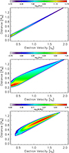 |
Fig. 13 Top:electron flux from a free-streaming electron beam with an initial power-law distribution in velocity after t = 5 s (v0 = 1010 cm s−1, 0.33 c). Middle and bottom: simulated electron flux and spectral energy density from a propagating electron beam with an initial power-law distribution, with a set-up described in Reid & Kontar (2015), after t = 5 s of propagation. |
6.3 TypeIII durations
The duration derived from a free-streaming electron beam at one point in space is dependent upon the velocity of the electrons that are considered. Between velocities v1 and v2, where v1 > v2, at some distance r from the injection site, the duration is simply
 (18)
(18)
From the LOFAR radio data, we can estimate the velocities v1 and v2 from the rise and decay velocities using the mean rise velocity v1 = 0.20 c and the mean decay velocity v2 = 0.15 c (Table 2), respectively.
Figure 14 shows the corresponding free-streaming duration as a function of plasma frequency assuming the Parker density model, that the emission is second harmonic, and that the electron beam starts at an altitude of 50 Mm, as has been found from fitting radio and X-ray data (Reid et al. 2014). The free-streaming duration using velocities v1 and v2 is incompatible with the mean radio burst durations, which have a significantly higher duration at all frequencies. This result is unsurprising given that the free-streaming approximation lacks the critical physical processes involved in radio burst production.
The duration derived assuming gas-dynamic theory will be constant as a function of frequency when we assume only one plateau with a constant velocity. However, if we assume that the front and back of the beam moves with plateau velocities u1 = (u1,max + u1,min)∕2 = 0.20 c and u2 = (u2,max + u2,min)∕ 2 = 0.15 c, respectively,the duration will increase as a function of decreasing frequency. An electron beam with a power-law distribution must propagate an instability distance before Langmuir waves are produced (Reid et al. 2011; Reid & Kontar 2013; Reid et al. 2014). The beam can be assumed to have propagated this instability distance under free-streaming conditions with velocities u1,max and u2,max. Velocity diffusion can then produce the plateaus u1 and u2 when Langmuir waves are generated. Given an instability distance rc, the corresponding duration of an electron beam can be found from
 (19)
(19)
We assume that rc = 4.13 × 1010 cm, (0.59 R⊙), which corresponds to a plasma frequency of 50 MHz in the Parker density model that would produce second-harmonic radio emission at 100 MHz. We can then fit the LOFAR durations using u1,min = 0.15 c and u2,min = 0.10 c, which gives u1,max = 0.24 c and u2,max = 0.2 c. The value of u2,min = 0.10 c is approximately 5.5 vte for a 2 MK plasma and u1,min > u2,min, as shown by the simulations in Figure 13.
We chose the value of u1,min and u2,min so that the corresponding values of  overlap the LOFAR durations, as shown in Fig. 14. Taking into account higher velocities during the instability distance will always reduce the duration with respect to the free-streaming approximation, when u1 = v1 and u2 = v2. However, it is important to note that our choice of u1,min and u2,min was arbitrary. Assuming a higher or lower u1,min will decrease or increase the value of
  accordingly for the same u1, u2. Similarly, increasing or decreasing rc will decrease or increase the value of
  accordingly. Although
  over-plots the radio data very well, the simple formula given in Eq. (19) is only an approximation and does not take into consideration many different physical mechanisms. It fits the radio data below 100 MHz well because it used the derived velocities of 0.20 c and 0.15 c that were estimated from the LOFAR data.
Numerical simulations of an electron beam can be used to estimate the corresponding durations at different frequencies. We can use the spectral energy density of the Langmuir waves as a proxy for the radio emission as the intensity will be related to the intensity of radio emission. For each frequency, we find the peak spectral energy density at each point in time. The duration is then calculated from the corresponding FWHM. Using the Langmuir waves as a proxy for radio emission ignores the effects of the wave-wave processes generating the radio waves from the Langmuir waves. We must therefore treat any results derived from this with care.
We used simulations described in Kontar (2001b); Reid & Kontar (2013, 2015), with initial conditions described by Table 3. We simulated two different initial beam densities nbeam = 104.5 cm−3 and nbeam = 105.0 cm−3. Varying the beam density changes the average velocities of the plateaus at the front of the beam. Higher beam densities allow electrons with higher velocities to produce Langmuir waves at the front of the electron beam. The velocity at the back of the electron beam is dominated by the thermal velocity.
The corresponding durations from the quasilinear simulations are shown in Fig. 14. The simulation with nbeam = 104.5 cm−3 resulted in a front velocity of u1 = 0.18 c and a back velocity of u2 = 0.14 c between plasma frequencies 35–15 MHz, relating to 70–30 MHz assuming second-harmonic emission. These velocities are similar to the LOFAR observations. There is a corresponding agreement between the durations derived from this simulation and the durations from the LOFAR observations. We note that the initial beam density was chosen such that u1 and u2 would be similar to the LOFAR observations.
The simulation with nbeam = 105.0 cm−3 resulted in a front velocity of u1 = 0.22 c and a back velocity of u2 = 0.14 c between the same plasma frequencies, which is faster than the LOFAR observations. The corresponding derived durations from the Langmuir waves are longer than the LOFAR observations. Whilst it is tempting to infer that higher beam densities result in increased durations, we note that the type III observations inferred that faster beams have shorter durations. To be consistent with this result, the FWHM of the radio emission must be related to the Langmuir waves generated by the fastest electrons. The wave-wave processes that convert Langmuir waves into radio waves could be responsible. Whilst simulating the radio waves from a propagating electron beam that had an initial Maxwellian distribution, Li et al. (2009) found that an increased beam density resulted in a decreased duration of second-harmonic emission. Additionally, the duration of any observed type III emission will be affected by the scattering of radio waves from source to observer, and this must be taken into account when composing a complete picture of electron beam transport.
The results from the simulations highlight why there is such a large standard deviation in the rise and decay times derived from the LOFAR type III bursts. Electron beams with varying properties can produce radio bursts with significantly different characteristics. Figure 14 suggests that the initial beam densities will play a significant role in determining the relevant velocity of electrons that drive the radio emission and might be one reason why the durations that we found with LOFAR are shorter than was found in previous observational reports. However, other different beam and background plasma parameters are also likely to influence the type III durations, including the beam spectral index, the background density profile, and thermal velocity.
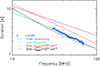 |
Fig. 14 Electron beam duration at different plasma frequencies, assuming second-harmonic emission. The free-streaming curve is calculated assuming v1 = 0.20 c and v2 = 0.15 c. The gas-dynamic fit is calculated assuming free-streaming to 100 MHz using u1,max = 0.24 c and u2,max = 0.19 c, then plateaus with average velocities u1 = 0.20 c and u2 = 0.15 c. The simulation with nbeam = 104.5 cm−3 (black) has u1 = 0.18 c and u2 = 0.14 c between 70–30 MHz. The simulation with nbeam = 105.0 cm−3 (red) has u1 = 0.22 c and u2 = 0.14 c between 70–30 MHz. |
Initial beam parameters for the electron beam injected into the solar corona.
7 Conclusions
We analysed the temporal and spectral profile of 31 isolated type III bursts that occurred between April–September 2015 observed with LOFAR. The increased resolution allowed us to characterise the rise and decay times, together with the drift rates and the bandwidth, in unprecedented detail. We found that the rise and decay times associated with the type III bursts increase as a function of decreasing frequency. Correspondingly, the FWHM duration of the type III bursts increases as a function of decreasing frequency, which is in line with previous observations, although the durations we found were slightly shorter than has previously been reported in the literature.
The drift rates of the type III bursts were simultaneously presented for the rise, peak, and decay times. Type III rise times resulted in higher magnitude drift rates than from decay times. Drift rates were used to infer the velocities of the front, middle, and back of the electron beams responsible for the radio emission. The mean velocities found over all radio bursts observed are 0.20 c, 0.17 c, and 0.15 c for the front, middle, and back of the beam, respectively. This highlights the long-standing belief that the electron beam elongates in space due to a range of velocities within the electron beam. It was particularly interesting that the difference between the velocities at the front and the back of the beam, that is, the rate of beam expansion in space, was proportional to the velocity of the middle of the beam. This can be interpreted as meaning that faster electron beams expand faster in space. However, radio-wave scattering and refraction strongly affect the observed type III burst characteristics. Specifically, it might induce a frequency-dependent delay, which could lead to a frequency-dependent apparent drift (Kontar et al. 2017). The decay of the burst might be more strongly affected by radio-wave propagation effects, which more strongly reduce the apparent speed at the back of the electron beam.
Although they move with one characteristic velocity, electron beams at one point in space are not mono-energetic, but are ensembles ofelectron at different energies. We showed the difference between the limiting cases of free-streaming electrons and the gas-dynamictheory, where electrons propagate in a single beam-plasma structure. We explained why neither theory is adequate for modelling the increasing duration of type III bursts as a function of decreasing frequency. Using simulations, we demonstrated that the different velocities at the front and back of the electron beam are likely caused by ensembles of electrons with different minimum and maximum velocities; the elongation of the beam being caused by the collection of electrons at the front having higher energies than at the back.
We showed that the duration inferred from the Langmuir waves is sensitive to the initial number density of the electron beam. Variation in the initial electron beam and the background coronal parameters are likely to be significant in explaining the shorter durations that we found in comparison to previous observations. However, the duration of type III bursts will also be affected by the wave-wave processes that convert Langmuir waves into radio waves and the scattering effects during radio-wave propagation. Our results increase the motivation of understanding all the plasma physics that governs the temporal and spectral type III profiles, so that these radio bursts can be better used to remote-sense electron beam properties in the solar corona and the inner heliosphere.
Acknowledgements
We acknowledge support from the STFC consolidated grant 173869-01. Support from a Marie Curie International Research Staff Exchange Scheme Radiosun PEOPLE-2011-IRSES-295272 RadioSun project is greatly appreciated. This work benefited from the Royal Society grant RG130642. This paper is based (in part) on data obtained with the International LOFAR Telescope (ILT) under project code LC3-012 and LC4-016. LOFAR (van Haarlem et al. 2013) is the Low Frequency Array designed and constructed by ASTRON. It has observing, data processing, and data storage facilities in several countries, that are owned by various parties (each with their own funding sources), and that are collectively operated by the ILT foundation under a joint scientific policy. The ILT resources have benefitted from the following recent major funding sources: CNRS-INSU, Observatoire de Paris and Université d’Orléans, France; BMBF, MIWF-NRW, MPG, Germany; Science Foundation Ireland (SFI), Department of Business, Enterprise and Innovation (DBEI), Ireland; NWO, The Netherlands; The Science and Technology Facilities Council, UK. We thank the staff of ASTRON, in particular Richard Fallows, for assistance in the set-up and testing for the solar LOFAR observations used.
References
- Abrami, A., Messerotti, M., Zlobec, P., & Karlicky, M. 1990, Sol. Phys., 130, 131 [NASA ADS] [CrossRef] [Google Scholar]
- Achong, A., & Barrow, C. H. 1975, Sol. Phys., 45, 467 [NASA ADS] [CrossRef] [Google Scholar]
- Alexander, J. K., Malitson, H. H., & Stone, R. G. 1969, Sol. Phys., 8, 388 [NASA ADS] [CrossRef] [Google Scholar]
- Alvarez, H., & Haddock, F. T. 1973a, Sol. Phys., 30, 175 [NASA ADS] [CrossRef] [Google Scholar]
- Alvarez, H., & Haddock, F. T. 1973b, Sol. Phys., 29, 197 [NASA ADS] [CrossRef] [Google Scholar]
- Aubier, M., & Boischot, A. 1972, A&A, 19, 343 [NASA ADS] [Google Scholar]
- Barrow, C. H., & Achong, A. 1975, Sol. Phys., 45, 459 [NASA ADS] [CrossRef] [Google Scholar]
- Carley, E. P., Vilmer, N., & Gallagher, P. T. 2016, ApJ, 833, 87 [NASA ADS] [CrossRef] [Google Scholar]
- Dulk, G. A., & Suzuki, S. 1980, A&A, 88, 203 [NASA ADS] [Google Scholar]
- Dulk, G. A., Goldman, M. V., Steinberg, J. L., & Hoang, S. 1987, A&A, 173, 366 [NASA ADS] [Google Scholar]
- Dulk, G. A., Leblanc, Y., Robinson, P. A., Bougeret, J.-L., & Lin, R. P. 1998, J. Geophys. Res., 103, 17223 [NASA ADS] [CrossRef] [Google Scholar]
- Elgaroy, O., & Lyngstad, E. 1972, A&A, 16, 1 [NASA ADS] [Google Scholar]
- Evans, L. G., Fainberg, J., & Stone, R. G. 1973, Sol. Phys., 31, 501 [NASA ADS] [CrossRef] [Google Scholar]
- Fainberg, J., Evans, L. G., & Stone, R. G. 1972, Science, 178, 743 [NASA ADS] [CrossRef] [Google Scholar]
- Holman, G. D., Aschwanden, M. J., Aurass, H., et al. 2011, Space Sci. Rev., 159, 107 [NASA ADS] [CrossRef] [Google Scholar]
- Hughes, M. P., & Harkness, R. L. 1963, ApJ, 138, 239 [NASA ADS] [CrossRef] [Google Scholar]
- Kontar, E. P. 2001a, Sol. Phys., 202, 131 [NASA ADS] [CrossRef] [Google Scholar]
- Kontar, E. P. 2001b, Comput. Phys. Commun., 138, 222 [NASA ADS] [CrossRef] [Google Scholar]
- Kontar, E. P., & Mel’Nik, V. N. 2003, Phys. Plasmas, 10, 2732 [NASA ADS] [CrossRef] [Google Scholar]
- Kontar, E. P., & Reid, H. A. S. 2009, ApJ, 695, L140 [NASA ADS] [CrossRef] [Google Scholar]
- Kontar, E. P., Lapshin, V. I., & Mel’Nik, V. N. 1998, Plasma Physics Reports, 24, 772 [Google Scholar]
- Kontar, E. P., Yu, S., Kuznetsov, A. A., et al. 2017, Nat. Commun., 8, 1515 [NASA ADS] [CrossRef] [Google Scholar]
- Krucker, S., Kontar, E. P., Christe, S., & Lin, R. P. 2007, ApJ, 663, L109 [Google Scholar]
- Krupar, V., Maksimovic, M., Santolik, O., et al. 2014, Sol. Phys., 289, 3121 [NASA ADS] [CrossRef] [Google Scholar]
- Krupar, V., Kontar, E. P., Soucek, J., et al. 2015, A&A, 580, A137 [NASA ADS] [CrossRef] [EDP Sciences] [Google Scholar]
- Li, B., & Cairns, I. H. 2013, J. Geophys. Res.: Space Phys., 118, 4748 [NASA ADS] [CrossRef] [Google Scholar]
- Li, B., & Cairns, I. H. 2014, Sol. Phys., 289, 951 [NASA ADS] [CrossRef] [Google Scholar]
- Li, B., Cairns, I. H., & Robinson, P. A. 2008, J. Geophys. Res.: Space Phys., 113, 6105 J. Geophys. Res.: Space Phys. [NASA ADS] [CrossRef] [Google Scholar]
- Li, B., Cairns, I. H., & Robinson, P. A. 2009, J. Geophys. Res.: Space Phys., 114, 2104 [NASA ADS] [Google Scholar]
- Li, B., Cairns, I. H., & Robinson, P. A. 2011, ApJ, 730, 20 [NASA ADS] [CrossRef] [Google Scholar]
- Mann, G., Jansen, F., MacDowall, R. J., Kaiser, M. L., & Stone, R. G. 1999, A&A, 348, 614 [NASA ADS] [Google Scholar]
- Markwardt, C. B. 2009, in Astronomical Data Analysis Software and Systems XVIII, eds. D. A. Bohlender, D. Durand, & P. Dowler, ASP Conf. Ser., 411 251 [NASA ADS] [Google Scholar]
- McLean, D. J., & Labrum, N. R. 1985, Solar Radiophysics: Studies of Emission From the Sun at Metre Wavelengths (Cambridge, UK: Cambridge University Press) [Google Scholar]
- Mel’Nik, V. N. 1995, Plasma Physics Reports, 21, 89 [NASA ADS] [Google Scholar]
- Mel’Nik, V. N., & Kontar, E. P. 1998, Phys. Scr., 58, 510 [NASA ADS] [CrossRef] [Google Scholar]
- Mel’Nik, V. N., Lapshin, V., & Kontar, E. 1999, Sol. Phys., 184, 353 [NASA ADS] [CrossRef] [Google Scholar]
- Mel’Nik, V. N., Konovalenko, A. A., Rucker, H. O., et al. 2011, Sol. Phys., 269, 335 [NASA ADS] [CrossRef] [Google Scholar]
- Morosan, D. E., Gallagher, P. T., Zucca, P., et al. 2014, A&A, 568, A67 [NASA ADS] [CrossRef] [EDP Sciences] [Google Scholar]
- Parker, E. N. 1958, ApJ, 128, 664 [Google Scholar]
- Poquerusse, M. 1977, A&A, 56, 251 [NASA ADS] [Google Scholar]
- Poquerusse, M., Bougeret, J. L., & Caroubalos, C. 1984, A&A, 136, 10 [NASA ADS] [Google Scholar]
- Ratcliffe, H., & Kontar, E. P. 2014, A&A, 562, A57 [NASA ADS] [CrossRef] [EDP Sciences] [Google Scholar]
- Ratcliffe, H., Kontar, E. P., & Reid, H. A. S. 2014, A&A, 572, A111 [NASA ADS] [CrossRef] [EDP Sciences] [Google Scholar]
- Reid, H. A. S., & Kontar, E. P. 2010, ApJ, 721, 864 [NASA ADS] [CrossRef] [Google Scholar]
- Reid, H. A. S., & Kontar, E. P. 2013, Sol. Phys., 285, 217 [NASA ADS] [CrossRef] [Google Scholar]
- Reid, H. A. S., & Kontar, E. P. 2015, A&A, 577, A124 [NASA ADS] [CrossRef] [EDP Sciences] [Google Scholar]
- Reid, H. A. S., & Kontar, E. P. 2017a, A&A, 606, A141 [NASA ADS] [CrossRef] [EDP Sciences] [Google Scholar]
- Reid, H. A. S., & Kontar, E. P. 2017b, A&A, 598, A44 [NASA ADS] [CrossRef] [EDP Sciences] [Google Scholar]
- Reid, H. A. S., & Ratcliffe, H. 2014, Res. Astron. Astrophys., 14, 773 [NASA ADS] [CrossRef] [Google Scholar]
- Reid, H. A. S., Vilmer, N., & Kontar, E. P. 2011, A&A, 529, A66 [NASA ADS] [CrossRef] [EDP Sciences] [Google Scholar]
- Reid, H. A. S., Vilmer, N., & Kontar, E. P. 2014, A&A, 567, A85 [NASA ADS] [CrossRef] [EDP Sciences] [Google Scholar]
- Reiner, M. J., & MacDowall, R. J. 2015, Sol. Phys., 290, 2975 [NASA ADS] [CrossRef] [Google Scholar]
- Riddle, A. C. 1972, Proc. Astron. Soc. Aust., 2, 98 [NASA ADS] [CrossRef] [Google Scholar]
- Riddle, A. C. 1974, Sol. Phys., 34, 181 [NASA ADS] [CrossRef] [Google Scholar]
- Ryutov, D. D., & Sagdeev, R. Z. 1970, Sov. J. Exp. Theor. Phys., 31, 396 [NASA ADS] [Google Scholar]
- Stappers, B. W., Hessels, J. W. T., Alexov, A., et al. 2011, A&A, 530, A80 [NASA ADS] [CrossRef] [EDP Sciences] [Google Scholar]
- Steinberg, J. L., Aubier-Giraud, M., Leblanc, Y., & Boischot, A. 1971, A&A, 10, 362 [NASA ADS] [Google Scholar]
- Suzuki, S., & Dulk, G. A. 1985, Bursts of Type III and Type V, eds. D. J. McLean, & N. R. Labrum, 289 [Google Scholar]
- Takakura, T., Naito, Y., & Ohki, K. 1975, Sol. Phys., 41, 153 [NASA ADS] [CrossRef] [Google Scholar]
- Tsybko, Y. G., 1989, Sov. Astron. Lett., 15, 453 [NASA ADS] [Google Scholar]
- van Haarlem, M. P., Wise, M. W., Gunst, A. W., et al. 2013, A&A, 556, A2 [NASA ADS] [CrossRef] [EDP Sciences] [Google Scholar]
- Vedenov, A. A. 1963, J. Nucl. Energy, 5, 169 [NASA ADS] [CrossRef] [Google Scholar]
All Tables
Velocities for the front, middle, and back of the electron beams using the Parker density model.
All Figures
|
Fig. 1 Top: background-subtracted type III flux profile around 48 MHz. The peak flux and HWHM points are shown as green circles. A Gaussian (red) and exponential (blue) fit are shown, together with their peak flux and HWHM. The Gaussian fit tracks the HWHM points in the data better, and the rise, peak, and decay times derived from the Gaussian fit are shown using the red dashed lines. Bottom: dynamic spectrum of the same burst. The drift of the rise, peak, and decay as a function of frequency are shown, together with the duration and bandwidth of the radio burst around 48 MHz. |
| In the text | |
|
Fig. 2 Mean rise time (top) and decay time (bottom) as a function of frequency for all the analysed type III bursts as found from the HWHM, tr and td, respectively. The top and bottom blue dashed lines show the spread of the data, found from the standard deviation. The red dashed line show the fits tr = (1.5± 0.1) f−0.77±0.14 and td = (2.2 ± 0.2) f−0.89±0.15 for frequency (per 30 MHz). For the decay time, the green and orange dashed lines show the fits from Evans et al. (1973) and Alvarez & Haddock (1973a), respectively, assuming a HWHM of td = τd log(2), from the derived exponential profiles τd. |
| In the text | |
|
Fig. 3 Top: asymmetry of the type III burst time profile along with the errors (in blue) on the rise and decay times. The red line highlights y = x. It is clear that the decay times are longer than rise times, with 77% of the time profiles having a longer decay time than rise time. Middle: mean rise time vs mean decay time, including the power-law fit to the data |
| In the text | |
|
Fig. 4 Mean duration as a function of frequency for all the type III bursts, as found from the FWHM. The blue dashed lines show the spread in the data from the standard deviation. The red dashed line shows the fit tD = (3.7 ± 0.2) f−0.86±0.11 for the frequency (per 30 MHz). The purple diamonds show the FWHM found from Aubier & Boischot (1972) and Barrow & Achong (1975). The purple pluses and triangles show the FWHM for fundamental and harmonic bursts, respectively, from Tsybko (1989). The purple squares show the FWHM for powerful (> 1000 SFU) type III bursts, from Mel’Nik et al. (2011). The orange and green dashed lines show the fit in frequency (per 30 MHz) of tD = 7.3f−1 reported by Suzuki & Dulk (1985) and tD = 6.2f−2∕3 reported by Elgaroy & Lyngstad (1972), respectively. |
| In the text | |
|
Fig. 5 Bandwidth Δf of the type III bursts as a function of peak frequency. |
| In the text | |
|
Fig. 6 Drift rate as a function of frequency for all type III bursts for the rise (top), peak (middle), and decay (bottom) times. The red dashed line shows the fitted power-law to the data. The orange dashed line shows the fit from (Alvarez & Haddock 1973b). The reduced one-sigma errors are obtained from the fitting uncertainties in the drift rate, taking into account the fitting uncertainties in t0. |
| In the text | |
|
Fig. 7 Drift rate as a function of duration for each type III burst. The red dashed line shows the linear fit to the data. |
| In the text | |
|
Fig. 8 Velocities derived from the rise, peak, and decay times of each type III burst assuming a constant velocity and the Parker density model. For almost all the bursts, the rise time is faster than the peak velocity, which in turn is faster than the decay velocity. The errors on the velocities from the fit are smaller than the symbols. |
| In the text | |
|
Fig. 9 Peak velocities as a function of durations for each type III burst. |
| In the text | |
|
Fig. 10 Length velocity (rate at which the electron beam length increases) against the peak velocity. The beam length velocity is derived from the difference between the velocities found from the rise and decay times. |
| In the text | |
|
Fig. 11 Left: velocities as a function of distance from the Sun for all the type III bursts using the Parker model (top) and the Dulk altitudes (bottom) after t = 5 s. The red line is a linear fit to the log of the velocity such that log10 (v) = ar + c. Right: Frequency and density profiles as a function of altitude for the Parker model (top) and Dulk model (bottom). |
| In the text | |
|
Fig. 12 Electron flux (left) and normalised spectral energy density (right) from an initial Gaussian electron beam with v0 = 1010cm s−1 (0.33 c). Top: free-streaming case with zero waves generated. Middle: gas-dynamic theory with electron beam velocities v < v0. Bottom: simulations using Eqs. (15), and (16). |
| In the text | |
|
Fig. 13 Top:electron flux from a free-streaming electron beam with an initial power-law distribution in velocity after t = 5 s (v0 = 1010 cm s−1, 0.33 c). Middle and bottom: simulated electron flux and spectral energy density from a propagating electron beam with an initial power-law distribution, with a set-up described in Reid & Kontar (2015), after t = 5 s of propagation. |
| In the text | |
|
Fig. 14 Electron beam duration at different plasma frequencies, assuming second-harmonic emission. The free-streaming curve is calculated assuming v1 = 0.20 c and v2 = 0.15 c. The gas-dynamic fit is calculated assuming free-streaming to 100 MHz using u1,max = 0.24 c and u2,max = 0.19 c, then plateaus with average velocities u1 = 0.20 c and u2 = 0.15 c. The simulation with nbeam = 104.5 cm−3 (black) has u1 = 0.18 c and u2 = 0.14 c between 70–30 MHz. The simulation with nbeam = 105.0 cm−3 (red) has u1 = 0.22 c and u2 = 0.14 c between 70–30 MHz. |
| In the text | |
Current usage metrics show cumulative count of Article Views (full-text article views including HTML views, PDF and ePub downloads, according to the available data) and Abstracts Views on Vision4Press platform.
Data correspond to usage on the plateform after 2015. The current usage metrics is available 48-96 hours after online publication and is updated daily on week days.
Initial download of the metrics may take a while.