| Issue |
A&A
Volume 613, May 2018
|
|
|---|---|---|
| Article Number | A72 | |
| Number of page(s) | 20 | |
| Section | Extragalactic astronomy | |
| DOI | https://doi.org/10.1051/0004-6361/201731988 | |
| Published online | 04 June 2018 | |
KMOS LENsing Survey (KLENS): Morpho-kinematic analysis of star-forming galaxies at z ~ 2★,★★
1
Observatoire de Genève, Université de Genève,
Ch. des Maillettes 51,
Versoix
1290,
Switzerland
e-mail: This email address is being protected from spambots. You need JavaScript enabled to view it.
2
CNRS, IRAP,
14 Avenue E. Belin,
31400
Toulouse,
France
3
European Southern Observatory,
Karl-Schwarzschild-Str. 2,
85748
Garching b. München,
Germany
4
SUPA, Institute for Astronomy, University of Edinburgh, Royal Observatory,
Edinburgh
EH9 3HJ,
UK
5
Dipartimento di Fisica e Astronomia, Università di Padova,
vicolo dellOsservatorio 2,
35122
Padova,
Italy
6
Univ. Lyon, Univ. Lyon 1, Ens de Lyon, CNRS, Centre de Recherche Astrophysique de Lyon UMR5574,
69230
Saint-Genis-Laval,
France
7
Departamento de Astrofísica y CC. de la Atmósfera, Universidad Complutense de Madrid,
28040
Madrid,
Spain
Received:
24
September
2017
Accepted:
17
January
2018
Abstract
We present results from the KMOS LENsing Survey (KLENS), which is exploiting gravitational lensing to study the kinematics of 24 star-forming galaxies at 1.4 < z < 3.5 with a median mass of log(M⋆∕M⊙) = 9.6 and a median star formation rate (SFR) of 7.5 M⊙ yr−1. We find that 25% of these low mass/low SFR galaxies are rotation-dominated, while the majority of our sample shows no velocity gradient. When combining our data with other surveys, we find that the fraction of rotation-dominated galaxies increases with the stellar mass, and decreases for galaxies with a positive offset from the main sequence (higher specific star formation rate). We also investigate the evolution of the intrinsic velocity dispersion, σ0, as a function of the redshift, z, and stellar mass, M⋆, assuming galaxies in quasi-equilibrium (Toomre Q parameter equal to 1). From the z − σ0 relation, we find that the redshift evolution of the velocity dispersion is mostly expected for massive galaxies (log(M⋆∕M⊙) > 10). We derive a M⋆ − σ0 relation, using the Tully–Fisher relation, which highlights that a different evolution of the velocity dispersion is expected depending on the stellar mass, with lower velocity dispersions for lower masses, and an increase for higher masses, stronger at higher redshift. The observed velocity dispersions from this work and from comparison samples spanning 0 < z < 3.5 appear to follow this relation, except at higher redshift (z > 2), where we observe higher velocity dispersions for low masses (log(M⋆∕M⊙) ~ 9.6) and lower velocity dispersions for high masses (log(M⋆∕M⊙) ~ 10.9) than expected. This discrepancy could, for instance, suggest that galaxies at high redshift do not satisfy the stability criterion, or that the adopted parametrization of the specific star formation rate and molecular properties fail at high redshift.
Key words: galaxies: high-redshift / galaxies: kinematics and dynamics / galaxies: evolution
Based on KMOS observations made with the European Southern Observatory VLT/Antu telescope, Paranal, Chile, collected under the program ID No. 095.A-0962(A)+(B).
The reduced datacubes (FITS files) are only available at the CDS via anonymous ftp to cdsarc.u-strasbg.fr (130.79.128.5) or via http://cdsarc.u-strasbg.fr/viz-bin/qcat?J/A+A/613/A72
© ESO 2018
1 Introduction
The kinematics of star-forming galaxies (SFGs) are known to provide key information about their fundamental properties. Studies of SFGs in the local Universe have shown that rotation curves are a powerful tool to understand their structure, mass distribution, dynamics, formation, and interactions (e.g., Persic et al. 1996; Sofue & Rubin 2001; Glazebrook 2013). Several scaling relations between these physical properties have now been established, for example, the empirical relation between luminosity or mass and rotation velocity of the disk, known as the Tully–Fisher relation (e.g., Tully & Fisher 1977; Pizagno et al. 2007; Courteau et al. 2007; Reyes et al. 2011). By studying the evolution of such scaling relations, we can gain insight into the physical conditions of high redshift galaxies.
Using near-infrared instruments, it has become possible to study the kinematics of galaxies at a particularly interesting epoch, around z ~ 2, when the cosmic star formation rate (SFR) density is at its peak and the mass assembly of galaxies is rapid (e.g., Madau et al. 1998; Pérez-González et al. 2005; Li 2008). Several large surveys (e.g. HiZELS, SINS/zC-SINF, MASSIV, KMOS3D, KROSS) of spatially-resolved ionized gas kinematics (including velocity gradients, velocity dispersion profiles, and dynamical masses), star formation, and physical properties (metallicity gradients, excitation) of SFGs at 0.8 < z < 2.7 have been undertaken with the integral field unit (IFU) spectrographs SINFONI/VLT, KMOS/VLT, and OSIRIS/Keck II (e.g., Förster Schreiber et al. 2009; Epinat et al. 2012; Sobral et al. 2013b; Wisnioski et al. 2015; Stott et al. 2016).
Overall, these surveys reveal that the majority (60–70%) of the resolved high redshift galaxies are rotation-dominated, while a minority of galaxies consist of merging systems and more compact, velocity-dispersion-dominated objects. The morphologies of these objects are observed to be more compact, clumpy, or irregular than at low redshift even if a rotating disk is observed. An increase of the intrinsic velocity dispersion with redshift is observed and is believed to be related to the higher gas fractions observed at high redshift (e.g., Law et al. 2009; Daddi et al. 2010; Geach et al. 2011; Tacconi et al. 2013; Saintonge et al. 2013; Sargent et al. 2014; Genzel et al. 2015; Dessauges-Zavadsky et al. 2015, 2017). In addition to larger gas reservoirs, this increase of random motions with redshift could be due to different effects such as diskinstabilities (e.g., Bournaud 2016; Stott et al. 2016) or an increase of the accretion efficiency (Law et al. 2009). The Tully–Fisher relation at high redshift is still debated, since Harrison et al. (2017) find a relation at z ~ 0.9 consistent with the local Universe, while a redshift evolution from z = 0 is obtained for two samples at z ~ 0.9 and z ~ 2.5 by Übler et al. (2017).
Clearly, these near-infrared studies have revolutionized our understanding of SFGs at z ~ 2. However, the picture is still incomplete, as the spatially-resolved surveys at high redshift remain limited to fairly massive galaxies (log (M⋆∕M⊙) ≳ 10) with large star formation rates (SFR ≳ 30 M yr−1), whereas the majority of galaxies at this epoch have a lower mass and SFR. Indeed, the characteristic mass M⋆ is known to be log(M⋆∕M⊙) ~ 10.3 at z ~ 2 (Ilbert et al. 2013) and both the Hα and infrared luminosity functions show that the characteristic SFR⋆ is between 30 and 60 M⊙ yr−1 (Sobral et al. 2013a; Burgarella et al. 2013). Studying galaxies with log(M⋆∕M⊙) < 10.3 at z ~ 1.5–2, the progenitors of the Milky Way, is essential to gain further evolutionary insights (Behroozi et al. 2013; Haywood et al. 2013).
Recent studies have investigated low mass galaxies at z < 2 with VLT/MUSE and VLT/KMOS (Contini et al. 2016; Swinbank et al. 2017). Gnerucci et al. (2011) and Turner et al. (2017) have used deep observations with VLT/SINFONI and VLT/KMOS to obtain a sample of low mass galaxies at z ~ 3.5. Another way to extend these studies to more numerous low mass and/or low SFR galaxies is by exploiting gravitational lensing, which allows us to probe below the knee of the luminosity function with current instrumentation. Already several studies have used this powerful tool to study kinematics (Jones et al. 2010; Livermore et al. 2015; Leethochawalit et al. 2016; Mason et al. 2017).
These lensed and deep surveys of low mass SFGs at high redshift confirm a high intrinsic velocity dispersion (σ ≳ 50 km s−1) until at least a redshift of 3.5 (Gnerucci et al. 2011; Livermore et al. 2015; Leethochawalit et al. 2016; Mason et al. 2017; Turner et al. 2017). Simulations have also shown that an increase of the dispersion is expected for Milky Way progenitors at least until a redshift of 1.2 (Kassin et al. 2014).
Overall, these low mass SFG surveys report a rotation-dominated fraction significantly lower (< 50%) than previous studies based on more massive galaxies. Recent simulations of galaxies in the local Universe have shown that the fraction of rotation-dominated galaxies is expected to increase with stellar mass (El-Badry et al. 2018). In this study, at log (M⋆∕M⊙) < 8, very few galaxiesare supported by rotation and none of them have a rotation curve which is flattened by rotation. At 8 < log(M⋆∕M⊙) < 10, both dispersion- and rotation-supported galaxies are obtained, and at 10 < log(M⋆∕M⊙) < 11 all the galaxies form a disk dominated by rotation. Observations in the local Universe are in good agreement with this picture, since a largediversity in the morphology and kinematics of low mass galaxies has been reported (e.g., Walter et al. 2008; Ott et al. 2012; Roychowdhury et al. 2013; Simons et al. 2015).
Nevertheless, the mass dependence on the rotation-dominated fraction and intrinsic velocity dispersion needs to be established from observations at high redshift, prompting us to carry out the KMOS LENsing Survey (KLENS). The goal of this survey is to extend existing near-infrared spectroscopic surveys using gravitational lensing to more numerous and typical galaxies at z ~ 2 with low mass (log (M⋆∕M⊙) ~ 9.5) and/or SFR (SFR < 30 M⊙ yr−1).
The paper is organized as follows. Section 2 describes our sample selection, observations, data reduction, and comparison samples. In Sect. 3, we explain measurements of the integrated properties and the SED fitting technique used to derive the stellar mass and the star formation rate. The morphological analysis of our sample is described in Sect. 4. Section 5 presents the kinematics and classification adopted in our work. Section 6 presents a discussion on the fraction of rotation-dominated galaxies and the evolution of the kinematic properties, specifically the intrinsicvelocity dispersion as a function of the redshift and stellar mass. We finally present our conclusions in Sect. 7.
In thispaper, we use a cosmology with H0 = 70 km s−1 Mpc−1, Ω M = 0.3, and Ω Λ = 0.7. When using values calculated with the initial mass function (IMF) of Salpeter (1955), we correct by a factor of 1.7 to convert to a Chabrier (2003) IMF.
2 Observations and data reduction
2.1 Sample selection and observations
We have selected our targets from two galaxy clusters from the CLASH program (Postman et al. 2012) and included in the Herschel Lensing Survey (HLS; Egami et al. 2010): MACS1206-08 and AS1063. For each cluster, the existing imaging, accurate magnification maps, and near-ultraviolet to far-infrared SED fits for all objects are available in the RAINBOW database (Pérez-González et al. 2008; Barro et al. 2011a,b), allowing us to select in an automated fashion galaxies based on their magnification, redshift, stellar mass, star formation rate, color-selection, and infrared luminosity. The criteria for our galaxy selection were:
-
a photometric redshift between 1.3 and 3.5 to detect the Hα or [OIII] emission lines in the H or K bands (Fig. 1, left panel);
an observed SFR higher than 10 M⊙ yr−1 to ensure a 5σ detection of Hα or [OIII];
-
an SFR corrected for magnification (SFR/μ) below 30 M⊙ yr−1 or a stellar mass corrected for magnification (M⋆∕μ) below 1010 M⊙, to extend existing near-infrared spectroscopic surveys below the current observational limits;
a magnification of μ ~ 1.5–4 and therefore galaxies located away from the critical lines to avoid effects caused by differential magnification within the object. In these seeing-limited data, the shear introduced by weak lensing is also negligible and does not affect the kinematics.
We initiated KLENS in 2015 in P95 with the K band Multi Object Spectrograph (KMOS; Sharples et al. 2013). KMOS has 24 arms of 14 × 14 spaxels. Each spaxel has 0.2′′ × 0.2′′, which gives a global field of view of 2.8′′× 2.8′′ for each arm. Observations were carried out in the H and K bands, which have a typical spectral resolution of R ~ 4000 and R ~ 4200, respectively.Each pointing had an exposure time of 300 s and we used an object-object-sky-object-object dither pattern. The sky frames were obtained by applying an offset to a clear sky position. The observations were taken in good conditions with a seeing around 0.6′′ in the H and K bands. The total on-source exposure time in the H band were 2.3 h for both clusters. In the K band, the targets were observed during 8 h and 10 h on-source for MACS1206-08 and AS1063, respectively.
Sixty different galaxies in MACS1206-08 and AS1063 have been observed. For these 60 galaxies, 19 at z ~ 2.2 were observed in both H and K bands, 21 at z ~ 3.0 were observed only in the K band, and 20 at z ~ 1.5 only in the H band. Figure 1 (left panel) presents the photometric redshifts of the observed galaxies.
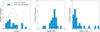 |
Fig. 1 Histograms of the redshift (left panel), stellar mass (middle panel), and star formation rate derived from the SED fitting (right panel) for the galaxies detected in our sample. The values are all lensing-corrected. |
2.2 Datareduction
The data reduction was performed primarily using the official KMOS ESOREX/SPARK pipeline (Davies et al. 2013), with the addition of custom Python scripts as described in detail in Turner et al. (2017). Each object frame (i.e., containing the science objects) was reduced individually using the sky frame nearest to it in time. The subtraction of the sky background was enhanced by using the SKYTWEAK optional routine within the ESOREX/SPARK pipeline. This routine performs a flux scaling of the individual OH sky-lines families to match the data, as well as a spectral shift to account for any wavelength miscalibration between object and sky frame (Davies et al. 2013).
Each sky-subtracted object frame was flux calibrated by using observations of a standard star taken the same night (before or after the science observations). The individual 300 s exposures where then stacked using a clipped average, providing a flux- and wavelength-calibrated datacube for every object. These cubes were used to create velocity maps and to extract one-dimensional spectra for the analysis presented here.
2.3 Comparison samples
In what follows, we summarize the different surveys we use for comparison in this work. We extract, from all the surveys mentioned below, the stellar mass, SFR (both corrected for Chabrier (2003) IMF), the redshift, velocity dispersion, and kinematic classification, when publicly available.
Livermore et al. (2015) present the kinematics of 12 gravitationally-lensed galaxies at 1 < z < 4 with 8.6 < log(M⋆∕ M⊙) < 10.8 (median of 9.4) and SFRs between 0.8 and 40 M⊙ yr−1. Leethochawalit et al. (2016) discuss the kinematics of 11 lensed galaxies at 1.4 < z < 2.5 with a mass range of 9.0 < log(M⋆∕M⊙) < 9.6 and SFRs between 5 and 250 M⊙ yr−1. The KMOS Lens-Amplified Spectroscopic Survey (KLASS) by Mason et al. (2017) uses gravitational lensing to study the kinematics of 25 galaxies at 0.7 < z < 2.3 with 7.8 < log(M⋆∕M⊙) < 10.5 (median of 9.5) and SFRs between 0.1 and 110 M⊙ yr−1. We use these three lensed surveys mainly to increase the number of galaxies in our sample, since these lensed galaxies have similar redshifts, stellar masses, and star formation rates to galaxies in KLENS. These three surveys, in addition to KLENS, will be referred to as the lensed surveys.
Moreover, for comparison at lower and higher redshifts, we use the data of Contini et al. (2016) obtained with MUSE (MUSE Hubble Deep Field South – HDFS) and Turner et al. (2017) obtained with KMOS (KMOS Deep Survey – KDS). Contini et al. (2016) study 28 galaxies at 0.2 <z < 1.4 in the mass range of 7.9 <log(M⋆∕M⊙) < 10.8 (median of 9.1) and SFRs between 0.01 and 80 M⊙ yr−1. Turner et al. (2017) present the kinematics of 38 resolved field galaxies at 3.0 <z < 3.8 in the stellar mass range 9.0 <log(M⋆∕M⊙) < 10.5 (median of 9.7) and SFRs between 4 and 175 M⊙ yr−1.
We finally also consider the commonly used surveys MUSE-KMOS (Swinbank et al. 2017), AMAZE (Gnerucci et al. 2011), MASSIV (Epinat et al. 2012), KMOS3D (Wisnioski et al. 2015), and SINS (Förster Schreiber et al. 2009). All these surveys have been summarized in the recent work of Turner et al. (2017).
3 Measurements
3.1 Detection of emission lines
We have setup a systematic way to detect emission lines in datacubes since the spectroscopic redshift of most of our targets was unknown. We initially use the Line Source Detection and Cataloguing software (LSDcat; Herenz & Wisotzki 2017). This software was first developed for large field of view IFUs like VLT/MUSE, but is also applicable to datacubes from VLT/KMOS. LSDcat allows us to detect the objects in our sample with the highest signal-to-noise ratio. However, the noisy datacubes we obtained prevent us from detecting weak emission lines with this technique.
Most ofthe detections have been made by fixing a central spaxel, corresponding spatially to the peak of HST emission, and creating a unique spectrum by summing all the spaxels inside a radius of 2 (0.4′′) and 5 (1.0′′) spaxels. The skylinesare also masked after the creation of these spectra. In this way, we get two spectra for each target to inspect visually. The 0.4′′ spectrum allows us to detect emission lines from more compact galaxies and the 1.0′′ spectrum allows us to detect more diffuse or extended galaxies.
We detect Hα or [OIII] emission lines in 24 targets out of 60 (i.e., 40% detection rate) from the galaxy clusters AS1063 and MACS1206-08. Two of these detected targets are observedin both H and K bands, 17 are detected in the H band, and five are detected in the K band only. We detect in addition to Hα and/or [OIII] the [NII] emission line in one galaxy and Hβ in three galaxies, but these lines are faint and only visible in the integrated spectra. The detected emission lines are summarized in Table 1.
We do not detect any emission line for the remaining 36 targets. The median H band magnitude of targets with non-detections is 23.4 compared to 23.0 for those with detections, which means that our low detection rate is not due to the detection limit. The low detection rate is likely due to a combination of various other effects. First, the strong and numerous skylines present in H and K bands, which can be at the same position as the emission lines. Second, we do not have any detection longwards of 2.3 μm in the K band, even for the galaxies which have a known spectroscopic redshift and where we expect a detection. This part of the K band shows a high level of noise in all our datacubes and it is probably due to the lower transmission towards the edges of the filters and the thermal noise of the instrument. As a consequence, the fractions of H and K bands lost are ~ 20% and ~ 60% respectively, which cannot explain completely our detection rate of 40%. It may also be that the photometric redshifts are not always accurate and therefore the emission lines are possibly outside the H and K bands. Finally, the Hα or [OIII] lines of the sources are perhaps weaker than expected, and hence undetected.
Integrated properties.
3.2 Redshift
We have determined spectroscopic redshifts using the wavelength of [OIII] or Hα emission lines from the one-dimensional spectra (Table 1). We obtain a median difference of 0.18 between zspec and zphot. When only one emission line is detected for a galaxy, we take the most likely redshift according to the probability density function (PDF). When we are not able to determine the redshift from the PDF, we perfom an SED fitting with both redshifts corresponding to [OIII] and Hα emission lines and take the redshift for which we obtain the best fit. Figure 1 (left panel) shows the redshift distribution of our sample.
The sources AS1063-1321 and AS1063-1152 are known to be multiple images of the same galaxy (Karman et al. 2015). We measure a redshift of z = 1.428, which is in good agreement with Karman et al. (2015; source 46, z = 1.428), Richard et al. (2014; source 2, z = 1.429), Balestra et al. (2013; source 6a, z = 1.429), and Johnson et al. (2014; source 6, z = 1.429). The redshiftz = 2.580 measured for the source AS1063-942 is also consistent with the redshift determined by Karman et al. (2015; source 48, z = 2.577).
The source AS1063-885 has been studied in detail by Vanzella et al. (2016) and Vanzella et al. (2017). They report in their work that this object is extremely blue and young, showing characteristics similar to a proto-globular cluster. They find a redshift of z = 3.1169, which is consistent with the redshift of z = 3.1171 we measure in this work.
The sources MACS1206-1472 and MACS1206-820 are also known as multiple images of the same galaxy (Zitrin et al. 2012). The redshift of 3.03 reported is also in good agreement with our measurement of z = 3.038.
3.3 Integrated properties
3.3.1 Line fitting
We first create an integrated spectrum for all the galaxies by summing the spaxels to maximize the signal-to-noise ratio. We fit 1000 Gaussian curves using a Monte Carlo technique perturbing the flux on each of the detected emission lines. The continuum level is determined by the average of all the pixels in a window of 50 around the center of theemission line. In this window, all the pixels affected by skylines are masked. When the window is populated by too many skylines, we extend itto 70. If the line is on the edge of the band, the window is cut before the edge and extended on the other side. As a result, we obtain an accurate systemic redshift, the Hα and/or [OIII] flux, the full width half maximum (FWHM), the velocity dispersion for each galaxy, and their associated uncertainties.
The Hα flux is measured for 17 galaxies in our sample.We use it to derive the star formation rate, SFRHα, following the Kennicutt (1998) equation:
 (1)
(1)
where the factor 1.7 is the correction for the Chabrier (2003) IMF, and μ is the magnification. Individual magnifications have been derived using the most up-to-date mass models of the clusters. The magnifications for AS1063 were derived by the CATS team as part of the Frontier Fields challenge (Richard et al. 2014). For MACS1206-08, we use the model described in Cava et al. (2018) constrained by many different regions of a giant arc in the cluster core. We have noted that the magnification values derived were similar to the ones previously derived by Zitrin et al. (2009, 2013) and obtained through the Hubble Space Telescope Archive as a high-end science product of the CLASH program (Postman et al. 2012). We obtain a mean and median fractional difference of 1.4 and 1.06, respectively for AS1063 and MACS1206-08, with a spread of 0.06, which means that our magnification values are slightly higher. Only the SFR and stellar mass are affected by the magnification.
We derive the integrated velocity dispersion, σint, by correcting the observed velocity dispersion, σobs, for the instrumental broadening, σinstr, which is obtained from the skylines
 (2)
(2)
These values are listed in Table 3. The median and average σint of our KLENS sources are 59 km s−1 and 64 km s−1, respectively.
Kinematic properties from fitted models.
Kinematic properties.
3.3.2 SED fitting
We adopteda modified version of the code Hyperz (Bolzonella et al. 2000; Schaerer & de Barros 2010) to perform the SED fit of the photometric data of our sources. In practice we use the 15 HST bands from the CLASH survey reaching from the bluest (WFC3 UVIS F225W) to the reddest filter (WFC3 IR F160W) plus the IRAC photometry at 3.6 and 4.5 μm. The photometry was taken from the RAINBOW database (cf. Sect. 2.1), relying on a recent multiwavelength catalog from Rodriguez-Muñoz et al. (in prep.). For the SED fits we fixed the redshift to the spectroscopic value. We adopted the stellar tracks of Bruzual & Charlot (2003) at solar metallicity, close to the values expected for most of our galaxies, and for comparison with other studies. We assumed exponentially-declining star formation histories with timescales τ ≥ 300 Myr, including constant SFR. The age is a free parameter in the fits, assuming t > 50 Myr to avoid unphysically young solutions. Nebular emission was neglected in our default models as it was found not to affect significantly the resulting stellar masses; this enabled us to make meaningful comparisons with other analyses, which also neglect emission. The attenuation was described by the Calzetti et al. (2000) law and was varied from AV = 0 to a maximum value  . Since model assumptions made here are very similar to those of other studies (Förster Schreiber et al. 2009; Swinbank et al. 2017) used for comparison in this paper, they should allow meaningful relative comparisons between these parameters.
The main physical parameters of interest here, stellar mass and the current SFR, were derived from the best-fit SEDs. All results are rescaled to the Chabrier (2003) IMF. To estimate the uncertainties we carried out Monte Carlo simulations perturbing the photometry of the sources. Fitting 1000 realizations of each source allowed us to determine the probability distribution function of these parameters. The corresponding median values and 68% confidence range, corrected for gravitational magnification, are listed in Table 1 and presented in Fig. 1 (middle and right panels). Adopting lower metallicities could lead to somewhat higher masses (see, e.g., Yabe et al. 2009). The largest uncertainty in the SFR is the assumption of the star formation history and age prior (Schaerer et al. 2013; Sklias et al. 2014). Again, the assumed star formation histories are very similar to those of other studies (Förster Schreiber et al. 2009; Swinbank et al. 2017) used for comparison here.
Figure 2 presents the distribution of galaxies in our sample in the diagram of SFRSED as a function of stellar mass, color-coded as a function of ΔSFR, which is defined as ΔSFR = log(SFR∕SFRMS), namely the offset from the main sequence (MS) derived by Tomczak et al. (2016) for the redshift of each galaxy.
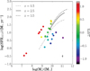 |
Fig. 2 Star formation rate from the SED fitting as a function of stellar mass for all the galaxies in our sample. The curves represent the main sequence of galaxies derived by Tomczak et al. (2016) for the redshifts of 1.5, 2.5, and 3.5. The color corresponds to the value of Δ SFR = log(SFR∕SFRMS), the offset from the main sequence. The typical error bar for individual points is shown in the lower right corner. |
4 Morphology
To further characterize the galaxies in our sample, an analysis of their morphology is required from high-resolution images. The morphology can give us information about the light profile and size as well as helping to distinguish galaxies in interaction, in an on-going merger, or with a clumpy disk. A visual inspection of the HST images shows that our sample includes a large variety of objects, such as compact galaxies, clumpy galaxies, and disk-like galaxies (see Figs. A.1–A.2). However, it is impossible to resolve any smaller structure such as spiral arms or a bar. We use the HST images in the image plane since differential amplification is negligible in our galaxies. Indeed, we obtain a median relative differential amplification of 6% with a spread of 2% within our objects. The median absolute differential amplification is ~ 0.12, which is of the same order as the median error on the amplification of ~ 0.1.
To classify our galaxies in a systematic way, we use GALFIT to perform two-dimensional fitting of light profile on two-dimensional images (Peng et al. 2002). We focus on the available HST/WFC3 F160W near-infrared images, which trace the rest-frame optical to the near-UV depending on the redshift of the galaxy, to extract a single image for each galaxy. We take the largest region possible around the galaxy that is not contaminated by light from other galaxies. We adopt a similar approach to Van der Wel et al. (2012) and Wisnioski et al. (2015) by determining a single Sérsic model per galaxy. To obtain a better fit, Rodrigues et al. (2017) use a more complex approach with a Sérsic model for the bulge and an exponential profile for the disk.However, our sample includes a large diversity of morphology to which a single-Sérsic fit is most appropriate.
All parameters are free to vary during the fitting process. We obtain as a result morphological parameters such as the effective radius (Re), the position angle (PAmorph), the axis ratio (b∕a), and the Sérsic index (n) for each galaxy. The Sérsic index, which is an indication of the light profile, approaches in most cases an exponential profile rather than a Devaucouleurs profile (Sérsic 1963). The derived Re are discussed in Sect. 5.1 and Fig. 3.
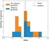 |
Fig. 3 Histogram of R/Re for the resolved galaxies of our sample, where R is the maximum radius where we get a measurement of the velocity and Re is the effective radius. Only galaxies for which it is possible to fit a light profile with GALFITare shown. The galaxies that do not show a velocity gradient are in orange and the galaxies for which it is possible to fit a kinematic model (velocity gradient) are presented in blue. |
5 Kinematics
5.1 Modeling
We performed Gaussian fits to the Hα or [OIII] emission line in individual spaxels to obtain the flux, velocity, and velocity dispersion maps. The results are shown in Figs. A.1–A.2. The spectroscopic redshift obtained from the integrated spectrum has been used to determine the central wavelength for the velocity maps. We used again a spectral window of 50 to determine the continuum and we masked all the skylines. We also determined the level of noise for each spaxel in the same spectral window. We binned spaxels 2 × 2 (0.4′′× 0.4′′) for the areawhere the noise was too high, but in most cases the new area is still too noisy (S∕N < 3). We rejected the spaxels where the signal-to-noise ratio is lower than two. We applied this method for all the galaxies resolved in our sample. The shear introduced by weak-lensing does not affect the kinematics since these low-magnification galaxies are seeing-limited.
To obtain the kinematics of our galaxies, we use two different approaches. First, we perfom fits with the GalPaK3D code, which directly fits a three-dimensional galaxy disk kinematic model to the three-dimensional datacubes (Bouché et al. 2015). This code has been used before on datacubes from VLT/MUSE (e.g., Contini et al. 2016), VLT/SINFONI (e.g., Schroetter et al. 2015), and VLT/KMOS (Mason et al. 2017). The three-dimensional model is convolved with the point spread function (PSF) and the line spread function (LSF) to derive kinematic properties such as the intrinsic velocity dispersion and rotation velocity, but also morphological properties like the inclination. The PSF in our case has been determined by the seeing obtained during the observations of stars from the acquisition image and the LSF has been measured from the skylines.
GalPaK3D is currently configured for an exponential, Gaussian, or De Vaucouleurs radial flux profile. We use an exponential profile, which is better-suited for our galaxies.
We adopt the arctangent function for the velocity profile (Courteau 1997), which has been used in many studies (e.g., Jones et al. 2010)
 (3)
(3)
where r is the radius, rt is the turnover radius, and υrot is the maximum rotation velocity.
GalPaK3D has ten parameters: the position of the center (x, y, λ), the disk half-light radius, R1∕2, the flux, the inclination, the position angle for the kinematics, PAkin, the turnover radius, rt, the maximum rotation velocity, υrot, and the intrinsic dispersion, σ0,galpak. We constrain the position center (x, y) in two spaxels according tothe flux map and λ in a window of twice the FWHM found with the integrated spectrum around the center of the emission line. The other parameters are free to vary. Since the number of spaxels with good signal-to-noise ratio in our galaxies is small, we have been able to fit only five galaxies with GalPaK3D.
For the other galaxies showing a velocity gradient in their velocity map but that are overfitted with GalPaK3D, we obtain a two-dimensional disk model following the arctangent function (Eq. (3)) using the Markov chain Monte Carlo (MCMC) method from Leethochawalit et al. (2016). This approach is used to fit the velocity map with the PSF convolved model. The spatial center is beforehand constrained to less than two spaxels and the inclination, the position angle for the kinematics, PA kin, the turnover radius, rt, and the maximum rotation velocity, υrot, are free to vary. The results of the 12 galaxies for which we have obtained model fits are shown in Fig. A.3 and are given in Table 2 with the velocity dispersion found by GalPaK3D when the kinematic fit with this tool converged.
The median value of R/Re in our sample is 1.2, where R is the maximum radius where we get a measurement of the velocity, and Re is the effectiveradius derived from a two-dimensional GALFIT fitting (Sect. 4). The histogram of R/Re for the galaxies in our sample is plotted in Fig. 3. Genzel et al. (2017) show that the rotation velocity, υrot, reaches a maximum between 1.3 Re and 1.5 Re, whereas in Lang et al. (2017) they obtain 1.65 Re by stacking more than 100 galaxies. Stott et al. (2016) take measurements of the rotation velocity at 2.2 Re, and Turner et al. (2017) at 2.0 Re, where the rotation curve already flattens. Therefore, a good signal-to-noise ratio at at least ~ 1.5 Re is needed to obtain an accurate rotation velocity.
In our sample, we obtain a radius R lower than the ~1.5 Re needed for many galaxies (see Fig. 3). As a result, there is a degeneracy between the different parameters in the kinematic model, and therefore our kinematic model results show large errors. In fact, we get a mean ratio of the rotation velocity from the models, υrot, and the maximum velocity observed from the rotation curve as large as ~ 29%, since the modeled rotation velocities are taken from the extrapolation of the rotation curve at large radii. Consequently, in what follows, we prefer to introduce a kinematic classification that does not refer to the uncertain υrot.
5.2 Empirical diagnostics
Another way to obtain information about the kinematics is by using the lower limit of the rotation velocity and the upper limitof the intrinsic velocity dispersion. For all the galaxies showing a gradient in the velocity field, we take the maximum and the minimum velocities observed on the major axis to obtain a lower limit on the rotation velocity:
 (4)
(4)
This value is not corrected for inclination and υobs,lim is then a lower limit (Table 3).
Different methods have been recently used to determine the intrinsic velocity dispersion and to correct for the beam smearing effect. Johnson et al. (2018), for example, measure the velocity dispersion in the outskirts of the galaxies, but also measure the median of all available spaxels. They afterwards apply beam smearing corrections that they derive from modeling the median values. Several studies use this first method and measure theintrinsic velocity dispersion where the beam smearing is expected to be negligible, namely in the outer regions on the major axis of galaxies (e.g., Förster Schreiber et al. 2009; Wisnioski et al. 2015). Recent tools have also been developed to model and extract the intrinsic galaxy dynamics directly from the datacubes like GalPaK3D (Bouché et al. 2015) and 3D-Barolo (Di Teodoro & Fraternali 2015). Moreover, several studies use the beam-smeared local velocity gradient to correct linearly the observed velocity (e.g., Stott et al. 2016; Mason et al. 2017).
In our case, the intrinsic velocity dispersion has been determined by using spaxels on the major axis showing the lowest values in the most outer regions of the galaxies to avoid beam-smearing effects as much as possible. Beam smearing is most significant for massive galaxies, galaxies with a high inclination, and compact galaxies (e.g., Newman et al. 2013; Burkert et al. 2016; Johnson et al. 2018). For our sample with a median mass of log (M⋆∕M⊙) = 9.6, a median inclination of ~45° and a median value of Re∕RPSF ~ 1.5, we expect that the beam smearing increases our measured velocity dispersions by less than ~ 10%, which is of the same order as the typical error on the measurements.
Since the beam smearing is expected to be negligible in our galaxies, and to be consistent with the measurements of Förster Schreiber et al. (2009) and Wisnioski et al. (2015), two of our largest comparison samples, we do not apply here any extra correction for the beam smearing after measuring the lowest velocity dispersion in the outskirts. We correct the value for instrumental broadening, which we measure from the skylines. We therefore obtain an upper limit on the velocity dispersion of
 (5)
(5)
The derived measurements are available in Table 3. We note that for the galaxies modeled with Galpak3D, the values obtained for σ0,lim are in good agreement with σ0,galpak since we obtain a difference of less than ~7%, indicating that our estimation of σ0 with σ0,lim is realistic.
5.3 Classification
Rotation-dominated galaxies have generally been classified using the ratio υrot ∕σ0 > 1 (e.g., Wisnioski et al. 2015). We also adopt this definition here, but in our case with υobs,lim and σ0,lim, which gives υobs,lim∕σ0,lim > 1. Since υobs,lim is a lower limit and σ0,lim is an upper limit, if υobs,lim∕σ0,lim > 1, one also has υrot∕σ0 > 1 by definition.
We divide our galaxies into four kinematic classes:
(1) Rotation-dominated: All galaxies with υobs,lim∕σ0,lim > 1 and with no evidence of disturbance in the dispersion map to avoid galaxies in interaction.
(2) Irregular rotators: All galaxies showing a gradient of velocity, but not classified as rotation-dominated. The classification is uncertain for these galaxies. Most of them show υobs,lim∕σ0,lim < 1. Some galaxies show υobs,lim∕σlim > 1, but also some signs of disturbance and interactions in their dispersion maps (see Figs. A.1–A.2).
-
(3) Non-rotators: No gradient in the velocity map is observed, objects are clumpy, compact, or with an irregular velocity map.
-
(4) Unresolved: Three galaxies in our sample are not resolved.
The position angle can also be an important indicator to classify the kinematics of galaxies. Rodrigues et al. (2017), Wisnioski et al. (2015), and several other studies suggest a large discrepancy between the position angle obtained from the morphology and kinematics is an indication of clumpy structure or interaction. A difference in |PA kin −PAmorph| = ΔPA up to 30° is usually tolerated. We find a mean and median of 23° and 10° with a spread of 7.5° respectively, meaning most of the galaxies in our sample are aligned (among the 12 objects with measured PA kin values). We have only three1 objects where ΔPA is clearly higher than 30°. One of these galaxies is classified as rotation-dominated and the other two as irregular.
A summary of our kinematic classification for each galaxy in KLENS can be found in Table 4. We see a velocity gradient in 12 galaxies. The flat part of the rotation curve is reached in only one galaxy and a peak of dispersion is seen in only two galaxies. The classification of Förster Schreiber et al. (2009), referred to afterwards as FS, is based on the criteria υobs,lim∕σint > 0.4 for rotation-dominated galaxies andυobs,lim∕σint < 0.4 for dispersion-dominated galaxies. Finally, the last column gives our final classification.
From our classification, we obtain a rotation-dominated galaxy fraction of ~ 25% (only resolved galaxies). Using the FS classification, we find a fraction of ~ 40% as rotation-dominated and a fraction of ~15% as dispersion-dominated. Adding the ΔPA criterion, the fractions of rotation-dominated galaxies become 15% and 30% for our classification and FS classification, respectively.Clearly, the choice of the classification has a big impact on the fraction and is important in the comparison with other samples, especially for small samples.
6 Discussion
6.1 Fraction of rotation-dominated galaxies
We find a fraction of rotation-dominated galaxies of 25–40% for our galaxies with low mass and/or low SFR. From the literature, we know that a low fraction is also observed in recent surveys studying low masses at high redshift such as Turner et al. (2017) with 35%, Leethochawalit et al. (2016) with 36%, and Gnerucci et al. (2011) with 30%. Mason et al. (2017) also obtain a fraction of only 12% when using strict criteria, but the fraction becomes ~ 60% when adding more irregular rotators. Contini et al. (2016) and Livermore et al. (2015) claim that up to 50% of their analysed galaxies are rotation-dominated. Other surveys studying more massive galaxies at 0.8 < z < 2.5 obtained a higher fraction. Förster Schreiber et al. (2009), Wisnioski et al. (2015), and Stott et al. (2016) find a fraction of ~ 75–80%, while Epinat et al. (2012) obtain 65%. A dependence between the mean redshift of the surveys and the rotation-dominated fraction has been observed in recent studies (e.g., Stott et al. 2016; Simons et al. 2017; Turner et al. 2017), but are there other physical parameters which drive the observed fractions of rotation-dominated galaxies?
To investigate this question, we combine our data with the comparison samples listed above (Sect. 2.3), which have publicly-available information needed to discriminate rotation-dominated galaxies from other types (e.g., dispersion-dominated, merger, no velocity gradient).
Figure 4 presents the respective histograms of the stellar mass, SFR, and Δ SFR (when available) for the galaxies classified as rotation-dominated with respect to other types. In the SINS sample the ratio υobs ∕σint > 0.4 is used as a criterion for rotation-dominated, while in the other surveys mentioned we classify the galaxies with υrot ∕σ0 > 1 as rotation-dominated.
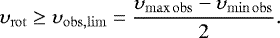
For all the surveys combined, we obtain a median mass of log (M⋆∕M⊙) = 9.73 with a spread of 0.14 and 9.36 with a spread of 0.17 for rotation-dominated galaxies and other types, respectively (Fig. 4, top panel). This indicates that massive galaxies are more often predominantly supported by ordered rotation than the low mass galaxies within a significance of 2σ.
This is in line with what we observe in our sample; the rotation-dominated galaxies seem mostly to be the massive ones (see Tables 1 and 4) as found by simulations of galaxies in the local Universe (El-Badry et al. 2018). The same trend is visible when we combine the rotation-dominated galaxies with the irregular rotators and compare them with the non-rotators. For our small sample, this trend could also be a bias of the detection limit because the low mass galaxies are less luminous. Therefore, the outer regions are poorly detected, and we possibly do not see the rotationbehavior in these galaxies. Förster Schreiber et al. (2009) have also reported an increase in the fraction of rotators for the massive galaxies of their sample, which was targeting more massive galaxies (median of log (M⋆∕M⊙) ~ 10.4) at similar redshifts to our study(z ~ 1.5–2.5). Kassin et al. (2012) obtain similar results with the DEEP2 Survey, as well as Simons et al. (2016, 2017) for galaxies at z ~ 2 with masses of 109 –1011 M⊙.
No cleartrend is observed for log (SFR) with a median of 0.78 ± 0.11 and 0.70 ± 0.11 M⊙ yr−1 for rotation-dominated and other types, respectively (Fig. 4, middle panel). Finally, there is a trend for galaxies showing starburst or intense star formation (ΔSFR > 0.5) in Fig. 4 (bottom panel) to be more likely to be irregular than the galaxies on the main sequence (Δ SFR ~ 0) or the quenching galaxies (ΔSFR < 0).
 |
Fig. 4 Histograms of the stellar mass (top panel), SFR (middle panel), and Δ SFR (bottom panel), where ΔSFR = log(SFR∕SFRMS), normalized for the rotation dominated galaxies compared to other types. We combine our data with SINS (Förster Schreiber et al. 2009), Livermore et al. (2015), MUSE-HDFS (Contini et al. 2016), MUSE-KMOS (Swinbank et al. 2017), KLASS (Mason et al. 2017), and KDS (Turner et al. 2017). KLASS is considered for the mass only, no SFR is available. |
Kinematic classification.
6.2 Evolution of the kinematic properties
In recent studies, it has been pointed out that the velocity dispersion increases with redshift. Wisnioski et al. (2015) have suggested this trend could come mainly from the increase of the gas fraction with redshift, in the framework of the equilibrium model. They propose a model following this idea. The gas fraction can be expressed as
 (6)
(6)
where tdepl is the molecular gas depletion timescale and sSFR the specific star formation rate. The tdepl is given by
![Mathematical equation: \begin{equation*} t_{\mathrm{depl}}(z) = 1.5(1+z)^{\alpha} \, \, [\mathrm{Gyr}], \end{equation*}](/articles/aa/full_html/2018/05/aa31988-17/aa31988-17-eq8.png) (7)
(7)
where the exponent has been fixed at α = −1 in the case of Wisnioski et al. (2015) based on the work of Tacconi et al. (2013). More recently Genzel et al. (2015) and Dessauges-Zavadsky et al. (2017) obtained a shallower tdepl dependance on z, which we adopt in this work (α = −0.85).
Wisnioski et al. (2015) use the parametrization of the specific star formation rate determined at 0.5 < z < 2.5 by Whitaker et al. (2014),
![Mathematical equation: \begin{equation*}\mathrm{sSFR}(z, {M}_{\star}) = 10^{a({M}_{\star})}(1+z)^{b({M}_{\star})} \, \, {[\textrm{Gyr}^{-1}]}, \end{equation*}](/articles/aa/full_html/2018/05/aa31988-17/aa31988-17-eq9.png) (8)
(8)
with a(M⋆) and b(M⋆) defined as
where the stellar mass is valid for 9.2 < log(M⋆∕M⊙) < 11.2.
Finally, following the Toomre equilibrium criterion (Toomre 1964), one gets
![Mathematical equation: \begin{equation*}\sigma_0(z, {M}_{\star}) = \frac{\upsilon_{\mathrm{rot}} \, f_{\mathrm{gas}}(z, {M}_{\star}) \, Q_{\mathrm{crit}}}{a} \, \, {[\textrm{km \, s}^{-1}]}, \end{equation*}](/articles/aa/full_html/2018/05/aa31988-17/aa31988-17-eq12.png) (9)
(9)
where  is assumed for a disk with a constant rotation velocity and Qcrit = 1 for a quasi-stable disk as identified in many studies (e.g., Förster Schreiber et al. 2006, Genzel et al. 2011, Burkert et al. 2010).
Reyes et al. (2011) have constrained the Tully–Fisher relation for the local galaxies,
![Mathematical equation: \begin{equation*}\mathrm{log} \, \upsilon_{\mathrm{rot}}({M}_{\star}) = 2.127 + 0.278 \, ( \mathrm{log} \, {M}_{\star} - 10.10) \, \, {[\textrm{km \, s}^{-1}]}. \end{equation*}](/articles/aa/full_html/2018/05/aa31988-17/aa31988-17-eq14.png) (10)
(10)
Many studies try to understand and constrain the evolution of this relation at higher redshifts, but recent studies show disparate results (e.g., Straatman et al. 2017; Übler et al. 2017; Harrison et al. 2017). To obtain a relation of the velocity dispersion strictly as a function of the redshift and stellar mass, we can rewrite Eq. (9) replacing the rotation velocity υrot by the Tully–Fisher relation (Eq. (10)) assuming it does not evolve with redshift as
![Mathematical equation: \begin{equation*}\sigma_0(z, {M}_{\star}) \simeq 0.147464 \, {M}_{\star}^{0.278} \, f_{\mathrm{gas}}(z, {M}_{\star}) \, \, {[\textrm{km \, s}^{-1}]}, \end{equation*}](/articles/aa/full_html/2018/05/aa31988-17/aa31988-17-eq15.png) (11)
(11)
where fgas is given by Eqs. (6)–(8). From Eq. (11), we can study the relation between the velocity dispersion and redshift, the σ0 − z relation, at a fixed stellar mass, and the relation between velocity dispersion and stellar mass, the σ0 − M⋆ relation, at fixed redshift.
Figure 5 shows the predicted velocity dispersion as a function of redshift. The curves are defined from Eq. (11) where we fix log(M⋆∕M⊙) at 9.5, 10.0, 10.5, and 11.0. A relatively steep evolution is found for the higher mass model, whilst a shallower evolution is found as mass decreases. We include in this figure measures from the different surveys mentioned in Sect. 2.3. We divide the lensed surveys in three different redshift bins: z < 2, 2 < z < 3, and z > 3, since they include galaxies mostly at 1 < z < 3.5. The respective log(M⋆∕M⊙) mean values of the latter galaxies are 9.6, 9.4, and 10 for each redshift bin. The lensed surveys now allow us to test the observed trend of the dispersion as a function of redshift for the lower mass galaxies and add a significant number of galaxies, especially at z > 1.
We can see the values from the lensed surveys, as well as all the other surveys, are overall in good agreement with the theoretical curves (Eqs. (6)–(11)) at their corresponding mass, taking into account the spread of the measured values in each redshift bin. We have to keep in mind here that the values from the different samples have not been corrected in the same way for the beam smearing. The lensed surveys have several galaxies for which we measure an upper limit on σ0, which means that the obtained values could be higher than the intrinsic velocity dispersions. If we apply an extra correction for the beam smearing, we find that our measurements are still in agreement with the model since the expected corrections are small for low mass galaxies and the errors due to the spread of the values in each redshift bin are larger than the correction (see Sect. 5.2; e.g., Burkert et al. 2016; Johnson et al. 2018).
As a result, globally the observations follow well the evolution model and interpretation of the intrinsic velocity dispersion as a function of redshift proposed by Wisnioski et al. (2015). We can now push further the analysis and try to distinguish the evolution of massive galaxies compared to low mass galaxies.
The dispersion as a function of stellar mass is presented in Fig. 6. The solid lines assume the Tully–Fisher relation of Reyes et al. (2011) described by Eq. (11), where we fix the redshift at the mean values of each redshift bin: 0.75, 1.25, 2.25, and 3.3. The redshift bins are defined in the same way as in Fig. 5, except that we add z < 1 and 1 < z < 2 now that we combine all the surveys together and have many galaxies in these bins. The dashed lines at z = 2.25 and z = 3.3 use the Tully–Fisher relation obtained by Straatman et al. (2017) at 2.0 < z < 2.5, which is probably more appropriate for these redshifts,
![Mathematical equation: \begin{equation*}{\mathrm{log}} \, \upsilon_{\mathrm{rot}}({M}_{\star}) = 2.17 + 0.29 \, ( \mathrm{log} \, M_{\star} - 10.0) \, \, {[\textrm{km \, s}^{-1}]}. \end{equation*}](/articles/aa/full_html/2018/05/aa31988-17/aa31988-17-eq16.png) (12)
(12)
We thusobtain the σ0 − M⋆ relation by rewriting Eq. (9), this time using Eq. (12),
![Mathematical equation: \begin{equation*}\sigma_0(z, {M}_{\star}) \simeq 0.131669 \, {M}_{\star}^{0.29} \, f_{\mathrm{gas}}(z, {M}_{\star}) \, \, {[\textrm{km \, s}^{-1}]}. \end{equation*}](/articles/aa/full_html/2018/05/aa31988-17/aa31988-17-eq17.png) (13)
(13)
At z ≳ 1, the plotted curves predict lower intrinsic velocity dispersions for lower masses, and an increase for higher masses, stronger at higher redshift due to the rapid decrease of the gas fraction with stellar mass. At z ≲ 1, the curves predict lower intrinsic velocity dispersions for the highest masses.
We consider three stellar mass bins for the plotted samples, 8.9 < log(M⋆∕M⊙) < 9.9, 9.9 < log(M⋆∕M⊙) < 10.5, and log (M⋆∕M⊙) > 10.5. Globally, we find a clear trend showing higher dispersion at high redshift for low and high mass galaxies as expected. The mean dispersions of each stellar mass bin are in good agreement with the curves within their 1.5σ dispersion, except for galaxies with a mass of 8.9 < log(M⋆∕M⊙) < 9.9 and log(M⋆∕M⊙) > 10.5, which show a discrepancy at higher redshift with higher and lower velocity dispersions than expected from the above relations, respectively (discussion below).
To better appreciate what is going on, Fig. 7 presents histograms of the velocity dispersion for the same data as in Fig. 6, but we divide here the galaxies into two subsamples with high masses, log (M⋆∕M⊙) > 10.2, and low masses, log(M⋆∕M⊙) < 10.2. The redshift bins are defined in the same way as in Fig. 6, apart from the higher redshifts for which we combine all the galaxies at z > 2 in only one bin, since most of the low mass galaxies are at z > 3 while most of the high mass are between 2 < z < 3 (therefore we do not have enough low and high mass galaxies at high redshift to divide our sample into two different redshift bins).
At z < 1, we obtain a similar velocity dispersion median of 31 ± 3 km s−1 and 31 ± 8 km s−1 for the low and high mass galaxies, respectively (zmean ~ 0.75; Fig. 7, top panel). This is expected at this redshift since the relations derived from Eq. (11) have comparable values regardless of the mass. At 1 < z < 2, we obtain a median of the velocity dispersion of 35 ± 5 km s−1 and 52 ± 9 km s−1 for the low and high mass galaxies, respectively (zmean ~ 1.25; Fig. 7, middle panel). This result is in agreement with the σ0 − M⋆ relation andcan be explained by the redshift evolution obtained at this redshift range for high mass galaxies, yielding a more rapid increase in dispersion for high mass than low mass galaxies.
At z > 2, however, we obtain a median of 66 ± 9 km s−1 and 50 ± 8 km s−1 for the low and high mass galaxies, respectively, when from the σ0 − M⋆ relation we expect toobtain values of ~51 km s−1 and ~ 81 km s−1. Figure 7 (bottom panel), in addition to Fig. 6, supports the evidence that low and high mass galaxies at z > 2 do not seem to follow the established σ0 − M⋆ relations. The velocity dispersions found at high redshift seem to be higher than expected for low mass galaxies, and lower for high mass galaxies.
The beam-smearing effect could play a role in the results obtained here. Indeed, if the measured velocity dispersions are higher than the intrinsic velocity dispersion, it could explain why we obtain higher values compared to the curves in many cases (see the datapoints at redshifts of 0.75 and 1.25 in Fig. 6). However, it cannot explain the lower value of σ0 we obtain at z > 2 for the high mass galaxies, since a beam-smearing correction would have the effect of lowering the value even more and increasing the observed discrepancy.
The velocity dispersion discrepancy at high redshift could be caused by an observational bias. It is possible that we only observe the low mass galaxies that have the higher dispersions because they are the easier to measure. We also might not be probing a representative sample of galaxies, in terms of their physical properties, at this epoch. In fact, as mentioned before, in the histogram showing the redshift bin z > 2 (Fig. 7, bottom panel), most of the low mass galaxies are at z > 3 (zmean ~ 3.15) while the majority of the high mass galaxies are between 2 < z < 3 (zmean ~ 2.4).
As proposed by some studies (e.g., Übler et al. 2017), it is also possible that the Tully–Fisher relation evolves more strongly at higher redshift, which would cause an offset toward higher dispersion, as we see in Fig. 6 with the Tully–Fisher from Straatman et al. (2017). However, we observe this offset only for the low mass galaxies, while the galaxies with masses of 9.9 < log(M⋆∕M⊙) < 10.5 seem to be in better agreement with the σ0 − M⋆ relation from Eq. (11). Moreover, on the contrary, a stronger evolution of the Tully–Fisher relation does not solve the discrepancy of the observations at the high mass end. An evolution of the slope of the Tully–Fisher relation would also directly affect the slope of the σ0 − M⋆ relation.
Assuming the established relations (Eqs. (6)–(11)), the sSFR has been determined for a valid range of 0.5 < z < 2.5. Using the SFR-M⋆ relation of Tomczak et al. (2016), parametrized up to z = 4, we obtain slightly different curves than those shown in Fig. 6. The velocity dispersions obtained for massive galaxies (log (M⋆∕M⊙) > 10.5) are quasi-constant at z > 2, with lower predicted values. However, the predicted velocity dispersions are still not low enough to be consistent with the observed velocity dispersions at this redshift.
The disagreement between data and the model at z > 2 could be an indication that the model with Qcrit = 1 fails for galaxies in these redshift and/or mass bins. A value of Qcrit > 1 would be necessary to be in agreement with the high velocity dispersion observed for low mass galaxies at z > 2, while a Qcrit < 1 would be necessary to obtain smaller velocity dispersion for high mass galaxies at the same redshift. A value of Qcrit < 1 usually is an indication of an unstable disk, while Qcrit > 1 indicates a stable disk (Genzel et al. 2011).
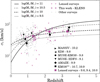 |
Fig. 5 Intrinsic velocity dispersion as a function of redshift. The curves are from Eq. (11) for log (M⋆ ∕M⊙) = 9.5, 10.0, 10.5, and 11.0. The magenta squares represent the mean velocity dispersions of the lensed surveys, which are the combination of our KLENS work, Livermore et al. (2015), Leethochawalit et al. (2016), and KLASS (Mason et al. 2017). The lensed surveys are divided into three redshift bins: z < 2, 2 < z < 3, and z > 3. The black symbols represent the mean velocity dispersions of the surveys listed at the lower right with their corresponding mean stellar masses. |
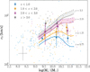 |
Fig. 6 Intrinsic velocity dispersion as a function of stellar mass. The solid and dashed lines are the σ0 − M⋆ relations from Eqs. (11) and (13) derived with the Tully–Fisher relation of Reyes et al. (2011) and Straatman et al. (2017), respectively. The redshifts correspond to 0.75, 1.25, 2.25, and 3.3, the mean values of each redshift bin. The circles represent the mean velocity dispersions of each stellar mass bin: 8.9 < log(M⋆∕M⊙) < 9.9, 9.9 < log(M⋆∕M⊙) < 10.5, and log (M⋆∕M⊙) > 10.5. The data are from the same surveys as in Fig. 5 when the mass is available. The typical error on individual datapoints is presented at the bottom left. |
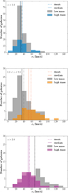 |
Fig. 7 Histograms of the intrinsic velocity dispersion for low and high masses at z < 1.0 (top panel), 1.0 < z < 2.0 (middle panel), and z > 2 (bottom panel). The low mass galaxies are defined as log(M⋆∕M⊙) < 10.2 and high mass as log(M⋆∕M⊙) > 10.2. The compilation is the same as in Fig. 6. |
7 Conclusions
We have presented KLENS, a survey exploiting gravitational lensing to study SFGs with low masses and/or SFR using the KMOS near-IR multi-object spectrograph at the VLT. We here report the first results using H and K band observations of two lensing clusters: AS1063 and MACS1206-08. We detect emission lines in 24 galaxies at 1.4 < z < 3.5 with a median mass of log(M⋆∕M⊙) = 9.6 and median SFR of 7.5 M⊙ yr−1. We show a morpho-kinematic analysis of our sample, and compare our kinematic classification with other surveys from the literature. We combine several surveys together to investigate the evolution of the intrinsic velocity dispersion as a function of the redshift and stellar mass, as well as the dependence between the fraction of rotation-dominated galaxies and integrated properties. The main results from this paper are summarized as follows:
There is a clear velocity gradient in 12 objects in our sample, while the 12 others are more compact, clumpy, or show irregular kinematics. For most of the objects showing a velocity gradient, we do not observe the flattening of the rotation curves or a peak in the velocity dispersion map at the kinematic center. Eight of them have ΔPA < 30° and two seem to show on-going interaction.
From our classification, we obtain a fraction of 25% of galaxies dominated by rotation. Using the criterion of Förster Schreiber et al. (2009), we obtain 40%.
When combining our data with other surveys, we find that the fraction of rotation-dominated galaxies appears to increase with stellar mass, while it decreases with a positive offset from the star formation main sequence.
We derive z − σ0 and M⋆ − σ0 relations using the Tully–Fisher relation and the equations previously obtained for the velocity dispersion by Wisnioski et al. (2015). We assume that galaxies are in quasi-equilibrium (Toomre Q parameter equal to one).
From the z − σ0 relation, we find a stronger redshift evolution of the velocity dispersion for massive galaxies. The observations are overall in good agreement with the z − σ0 relation corresponding to their mass.
-
From the M⋆ − σ0 relation, we obtain lower velocity dispersions for lower stellar masses, and an increase for higher masses, stronger at higher redshift. Observations are consistent with these relations, except at z > 2, where we observe higher velocity dispersion for low mass galaxies and lower velocity dispersions for high mass galaxies. This disagreement between theoretical curves and observations could suggest that the Tully–Fisher relation that we use is inadequate for this mass and/or redshift range. It could also indicate that the classical Toomre stability criterion is not satisfied at high redshift (with the Toomre Q parameter different from one), or that the adopted parametrization of the sSFR and molecular properties fail at high redshift.
Acknowledgements
This work has made use of the Rainbow Cosmological Surveys Database, which is operated by the Universidad Complutense de Madrid (UCM), partnered with the University of California Observatories at Santa Cruz (UCO/Lick,UCSC). We are very grateful to Tucker Jones and Nicha Leethochawalit for sharing their two-dimensional modeling codes. We also want to thank Mark Swinbank for advice on the data reduction and Nicolas Bouché for discussions on GalPaK3D. This work was supported by the Swiss National Science Foundation. MG is grateful to the Fonds de recherche du Québec – Nature et Technologies (FRQNT) for financial support. PGP-G acknowledges support from Spanish Government MINECO grants AYA2015-63650-P and AYA2015-70815-ERC.
Appendix A Kinematic maps
Figures A.1 and A.2 show the HST images, Hα or [OIII] flux, the velocity, and velocity dispersion maps of each galaxy of our sample. Figure A.3 presents the observed velocity maps, the velocity maps from the models, the rotation curves, and the velocity dispersion profiles of each galaxy showing a velocity gradient.
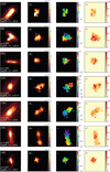 |
Fig. A.1 HST/WFC3 F160W near-infrared images, the Hα or [OIII] fluxin erg s−1 cm−1, the velocity, and velocity dispersion maps in km s−1 of galaxies from the cluster AS1063. The ellipses in the HST/WFC3 images represent the effective radii. |
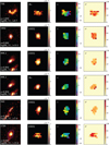 |
Fig. A.1 continued. |
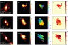 |
Fig. A.2 continued. |
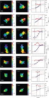 |
Fig. A.3 Observed velocity maps, velocity maps from the kinematic models, and rotation curves extracted on the major axis as indicated by the white solid lines on the maps. The blue circles and black solid line represent the curve extracted from the observed velocity maps and velocity maps from the model, respectively. The red dashed lines show the intrinsic rotation curves from the models. The vertical black solid lines indicate the value of the effective radius Re. The red circles and the horizontal black solid lines represent the velocity dispersion profile and the measured intrinsic velocity dispersion. The horizontal purple dashed lines indicate the intrinsic velocity dispersion obtained with GalPaK3D for five galaxies. |
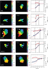 |
Fig. A.3 continued. |
References
- Balestra, I., Vanzella, E., Rosati, P., et al. 2013, A&A, 559, L9 [NASA ADS] [CrossRef] [EDP Sciences] [Google Scholar]
- Barro, G., Pérez-González, P. G., Gallego, J., et al. 2011a, ApJS, 193, 13 [NASA ADS] [CrossRef] [Google Scholar]
- Barro, G., Pérez-González, P. G., Gallego, J., et al. 2011b, ApJS, 193, 30 [NASA ADS] [CrossRef] [Google Scholar]
- Behroozi, P. S., Wechsler, R. H., & Conroy, C. 2013, ApJ, 770, 57 [NASA ADS] [CrossRef] [Google Scholar]
- Bolzonella, M., Miralles, J.-M., & Pelló, R. 2000, A&A, 363, 476 [NASA ADS] [Google Scholar]
- Bouché, N., Carfantan, H., Schroetter, I., Michel-Dansac, L., & Contini, T. 2015, AJ, 150, 92 [NASA ADS] [CrossRef] [Google Scholar]
- Bournaud, F. 2016, ASSL, 418, 355 [Google Scholar]
- Bruzual, G., & Charlot, S. 2003, MNRAS, 344, 1000 [NASA ADS] [CrossRef] [Google Scholar]
- Burgarella, D., Buat, V., Gruppioni, C., et al. 2013, A&A, 554, A70 [NASA ADS] [CrossRef] [EDP Sciences] [Google Scholar]
- Burkert, A., Genzel, R., Bouché, N., et al. 2010, ApJ, 725, 2324 [NASA ADS] [CrossRef] [Google Scholar]
- Burkert, A., Förster Schreiber, N. M., Genzel, R., et al. 2016, ApJ, 826, 214 [NASA ADS] [CrossRef] [Google Scholar]
- Calzetti, D., Armus, L., Bohlin, R. C., et al. 2000, ApJ, 533, 682 [NASA ADS] [CrossRef] [Google Scholar]
- Cava, A., Schaerer, D., Richard, J., et al. 2018, Nat. Astron., 2, 76 [Google Scholar]
- Chabrier, G. 2003, PASP, 115, 763 [NASA ADS] [CrossRef] [Google Scholar]
- Contini, T., Epinat, B., Bouché, N., et al. 2016, A&A, 591, A49 [NASA ADS] [CrossRef] [EDP Sciences] [Google Scholar]
- Courteau, S. 1997, AJ, 114, 2402 [NASA ADS] [CrossRef] [Google Scholar]
- Courteau, S., Dutton, A. A., van den Bosch, F. C., et al. 2007, ApJ, 671, 203 [NASA ADS] [CrossRef] [Google Scholar]
- Daddi, E., Bournaud, F., Walter, F., et al. 2010, ApJ, 713, 686 [NASA ADS] [CrossRef] [Google Scholar]
- Davies, R. I., Agudo Berbel, A., Wiezorrek, E., et al. 2013, A&A, 558, A56 [NASA ADS] [CrossRef] [EDP Sciences] [Google Scholar]
- Dessauges-Zavadsky, M., Zamojski, M., Schaerer, D., et al. 2015, A&A, 577, A50 [NASA ADS] [CrossRef] [EDP Sciences] [Google Scholar]
- Dessauges-Zavadsky, M., Zamojski, M., Rujopakarn, W., et al. 2017, A&A, 605, A81 [NASA ADS] [CrossRef] [EDP Sciences] [Google Scholar]
- Di Teodoro, E. M., & Fraternali, F. 2015, MNRAS, 451, 3021 [NASA ADS] [CrossRef] [Google Scholar]
- Egami, E., Rex, M., Rawle, T. D., et al. 2010, A&A, 518, L12 [CrossRef] [EDP Sciences] [Google Scholar]
- El-Badry, K., Quataert, E., Wetzel, A., et al. 2018, MNRAS, 473, 1930 [Google Scholar]
- Epinat, B., Tasca, L., Amram, P., et al. 2012, A&A, 539, A92 [NASA ADS] [CrossRef] [EDP Sciences] [Google Scholar]
- Förster Schreiber, N. M., Genzel, R., Lehnert, M. D., et al. 2006, ApJ, 645, 1062 [NASA ADS] [CrossRef] [Google Scholar]
- Förster Schreiber, N. M., Genzel, R., Bouché, N., et al. 2009, ApJ, 706, 1364 [NASA ADS] [CrossRef] [Google Scholar]
- Geach, J. E., Smail, I., Moran, S. M., et al. 2011, ApJ, 730, L19 [NASA ADS] [CrossRef] [Google Scholar]
- Genzel, R., Newman, S., Jones, T., et al. 2011, ApJ, 733, 101 [NASA ADS] [CrossRef] [Google Scholar]
- Genzel, R., Tacconi, L. J., Lutz, D., et al. 2015, ApJ, 800, 20 [NASA ADS] [CrossRef] [Google Scholar]
- Genzel, R., Schreiber, N. M. F., Übler, H., et al. 2017, Nature, 543, 397 [NASA ADS] [CrossRef] [Google Scholar]
- Glazebrook, K. 2013, PASA, 30, 56 [CrossRef] [Google Scholar]
- Gnerucci, A., Marconi, A., Cresci, G., et al. 2011, A&A, 528, A88 [NASA ADS] [CrossRef] [EDP Sciences] [Google Scholar]
- Harrison, C. M., Johnson, H. L., Swinbank, A. M., et al. 2017, MNRAS, 467, 1965 [NASA ADS] [CrossRef] [Google Scholar]
- Haywood, M., Di Matteo, P., Lehnert, M. D., Katz, D., & Gómez, A. 2013, A&A, 560, A109 [NASA ADS] [CrossRef] [EDP Sciences] [Google Scholar]
- Herenz, E. C.,& Wisotzki, L. 2017, A&A, 602, A111 [NASA ADS] [CrossRef] [EDP Sciences] [Google Scholar]
- Ilbert, O., McCracken, H. J., Le Févre, O., et al. 2013, A&A, 556, A55 [NASA ADS] [CrossRef] [EDP Sciences] [Google Scholar]
- Johnson, T. L., Sharon, K., Bayliss, M. B., et al. 2014, ApJ, 797, 48 [NASA ADS] [CrossRef] [Google Scholar]
- Johnson, H. L., Harrison, C. M., Swinbank, A. M., et al. 2018, MNRAS, 474, 5076 [NASA ADS] [CrossRef] [Google Scholar]
- Jones, T. A., Swinbank, A. M., Ellis, R. S., Richard, J., & Stark, D. P. 2010, MNRAS, 404, 1247 [NASA ADS] [Google Scholar]
- Karman, W., Caputi, K. I., Grillo, C., et al. 2015, A&A, 574, A11 [NASA ADS] [CrossRef] [EDP Sciences] [Google Scholar]
- Kassin, S. A., Weiner, B. J., Faber, S. M., et al. 2012, ApJ, 758, 106 [NASA ADS] [CrossRef] [Google Scholar]
- Kassin, S. A., Brooks, A., Governato, F., Weiner, B. J., & Gardner, J. P. 2014, ApJ, 790, 89 [NASA ADS] [CrossRef] [Google Scholar]
- Kennicutt, Jr., R. C. 1998, ARA&A, 36, 189 [Google Scholar]
- Lang, P., Förster Schreiber, N. M., Genzel, R., et al. 2017, ApJ, 840, 92 [NASA ADS] [CrossRef] [Google Scholar]
- Law, D. R., Steidel, C. C., Erb, D. K., et al. 2009, ApJ, 697, 2057 [NASA ADS] [CrossRef] [Google Scholar]
- Leethochawalit, N., Jones, T. A., Ellis, R. S., et al. 2016, ApJ, 820, 84 [NASA ADS] [CrossRef] [Google Scholar]
- Li, L.-X. 2008, MNRAS, 388, 1487 [NASA ADS] [CrossRef] [Google Scholar]
- Livermore, R. C., Jones, T. A., Richard, J., et al. 2015, MNRAS, 450, 1812 [NASA ADS] [CrossRef] [Google Scholar]
- Madau, P., Pozzetti, L., & Dickinson, M. 1998, ApJ, 498, 106 [NASA ADS] [CrossRef] [Google Scholar]
- Mason, C. A., Treu, T., Fontana, A., et al. 2017, ApJ, 838, 14 [NASA ADS] [CrossRef] [Google Scholar]
- Newman, S. F., Genzel, R., Förster Schreiber, N. M., et al. 2013, ApJ, 767, 104 [NASA ADS] [CrossRef] [Google Scholar]
- Ott, J., Stilp, A. M., Warren, S. R., et al. 2012, AJ, 144, 123 [NASA ADS] [CrossRef] [Google Scholar]
- Peng, C. Y., Ho, L. C., Impey, C. D., & Rix, H.-W. 2002, AJ, 124, 266 [NASA ADS] [CrossRef] [Google Scholar]
- Pérez-González, P. G., Rieke, G. H., Egami, E., et al. 2005, ApJ, 630, 82 [NASA ADS] [CrossRef] [Google Scholar]
- Pérez-González, P. G., Trujillo, I., Barro, G., et al. 2008, ApJ, 687, 50 [NASA ADS] [CrossRef] [Google Scholar]
- Persic, M., Salucci, P., & Stel, F. 1996, MNRAS, 281, 27 [NASA ADS] [CrossRef] [Google Scholar]
- Pizagno, J., Prada, F., Weinberg, D. H., et al. 2007, AJ, 134, 945 [NASA ADS] [CrossRef] [Google Scholar]
- Postman, M., Coe, D., Benítez, N., et al. 2012, ApJS, 199, 25 [NASA ADS] [CrossRef] [Google Scholar]
- Reyes, R., Mandelbaum, R., Gunn, J. E., Pizagno, J., & Lackner, C. N. 2011, MNRAS, 417, 2347 [NASA ADS] [CrossRef] [Google Scholar]
- Richard, J., Jauzac, M., Limousin, M., et al. 2014, MNRAS, 444, 268 [NASA ADS] [CrossRef] [Google Scholar]
- Rodrigues, M., Hammer, F., Flores, H., Puech, M., & Athanassoula, E. 2017, MNRAS, 465, 1157 [NASA ADS] [CrossRef] [Google Scholar]
- Roychowdhury, S., Chengalur, J. N., Karachentsev, I. D., & Kaisina, E. I. 2013, MNRAS, 436, L104 [NASA ADS] [CrossRef] [Google Scholar]
- Saintonge, A., Lutz, D., Genzel, R., et al. 2013, ApJ, 778, 2 [NASA ADS] [CrossRef] [Google Scholar]
- Salpeter, E. E. 1955, ApJ, 121, 161 [Google Scholar]
- Sargent, M. T., Daddi, E., Béthermin, M., et al. 2014, ApJ, 793, 19 [NASA ADS] [CrossRef] [Google Scholar]
- Schaerer, D., & de Barros S. 2010, A&A, 515, A73 [NASA ADS] [CrossRef] [EDP Sciences] [Google Scholar]
- Schaerer, D., de Barros S., & Sklias, P. 2013, A&A, 549, A4 [NASA ADS] [CrossRef] [EDP Sciences] [Google Scholar]
- Schroetter, I., Bouché, N., Péroux, C., et al. 2015, ApJ, 804, 83 [NASA ADS] [CrossRef] [Google Scholar]
- Sérsic, J. L. 1963, Boletín de la Asociación Argentina de Astronomía La Plata Argentina, 6, 41 [Google Scholar]
- Sharples, R., Bender, R., Agudo Berbel, A., et al. 2013, The Messenger, 151, 21 [NASA ADS] [Google Scholar]
- Simons, R. C., Kassin, S. A., Weiner, B. J., et al. 2015, MNRAS, 452, 986 [NASA ADS] [CrossRef] [Google Scholar]
- Simons, R. C., Kassin, S. A., Trump, J. R., et al. 2016, ApJ, 830, 14 [NASA ADS] [CrossRef] [Google Scholar]
- Simons, R. C., Kassin, S. A., Weiner, B. J., et al. 2017, ApJ, 843, 46 [NASA ADS] [CrossRef] [Google Scholar]
- Sklias, P., Zamojski, M., Schaerer, D., et al. 2014, A&A, 561, A149 [NASA ADS] [CrossRef] [EDP Sciences] [Google Scholar]
- Sobral, D., Smail, I., Best, P. N., et al. 2013a, MNRAS, 428, 1128 [NASA ADS] [CrossRef] [Google Scholar]
- Sobral, D., Swinbank, A. M., Stott, J. P., et al. 2013b, ApJ, 779, 139 [NASA ADS] [CrossRef] [Google Scholar]
- Sofue, Y., & Rubin, V. 2001, ARA&A, 39, 137 [NASA ADS] [CrossRef] [Google Scholar]
- Stott, J. P., Swinbank, A. M., Johnson, H. L., et al. 2016, MNRAS, 457, 1888 [NASA ADS] [CrossRef] [Google Scholar]
- Straatman, C. M. S., Glazebrook, K., Kacprzak, G. G., et al. 2017, ApJ, 839, 57 [NASA ADS] [CrossRef] [Google Scholar]
- Swinbank, A. M., Harrison, C. M., Trayford, J., et al. 2017, MNRAS, 467, 3140 [NASA ADS] [Google Scholar]
- Tacconi, L. J., Neri, R., Genzel, R., et al. 2013, ApJ, 768, 74 [Google Scholar]
- Tomczak, A. R., Quadri, R. F., Tran, K.-V. H., et al. 2016, ApJ, 817, 118 [NASA ADS] [CrossRef] [Google Scholar]
- Toomre, A. 1964, ApJ, 139, 1217 [NASA ADS] [CrossRef] [Google Scholar]
- Tully, R. B., & Fisher, J. R. 1977, A&A, 54, 661 [NASA ADS] [Google Scholar]
- Turner, O. J., Cirasuolo, M., Harrison, C. M., et al. 2017, MNRAS, 471, 1280 [NASA ADS] [CrossRef] [Google Scholar]
- Übler, H., Förster Schreiber, N. M., Genzel, R., et al. 2017, ApJ, 842, 121 [NASA ADS] [CrossRef] [Google Scholar]
- Van der Wel, A., Bell, E. F., Häussler, B., et al. 2012, ApJS, 203, 24 [NASA ADS] [CrossRef] [Google Scholar]
- Vanzella, E., De Barros, S., Cupani, G., et al. 2016, ApJ, 821, L27 [NASA ADS] [CrossRef] [Google Scholar]
- Vanzella, E., Calura, F., Meneghetti, M., et al. 2017, MNRAS, 467, 4304 [NASA ADS] [CrossRef] [Google Scholar]
- Walter, F., Brinks, E., de Blok, W. J. G., et al. 2008, AJ, 136, 2563 [NASA ADS] [CrossRef] [Google Scholar]
- Whitaker, K. E., Franx, M., Leja, J., et al. 2014, ApJ, 795, 104 [NASA ADS] [CrossRef] [MathSciNet] [Google Scholar]
- Wisnioski, E., Förster Schreiber, N. M., Wuyts, S., et al. 2015, ApJ, 799, 209 [NASA ADS] [CrossRef] [Google Scholar]
- Yabe, K., Ohta, K., Iwata, I., et al. 2009, ApJ, 693, 507 [NASA ADS] [CrossRef] [Google Scholar]
- Zitrin, A., Broadhurst, T., Umetsu, K., et al. 2009, MNRAS, 396, 1985 [NASA ADS] [CrossRef] [Google Scholar]
- Zitrin, A., Rosati, P., Nonino, M., et al. 2012, ApJ, 749, 97 [NASA ADS] [CrossRef] [Google Scholar]
- Zitrin, A., Meneghetti, M., Umetsu, K., et al. 2013, ApJ, 762, L30 [NASA ADS] [CrossRef] [Google Scholar]
There is also a fourth object, AS1063-732, for which it has been impossible to define ΔPA since the galaxy shows evident clumps in the HST image.
All Tables
All Figures
|
Fig. 1 Histograms of the redshift (left panel), stellar mass (middle panel), and star formation rate derived from the SED fitting (right panel) for the galaxies detected in our sample. The values are all lensing-corrected. |
| In the text | |
|
Fig. 2 Star formation rate from the SED fitting as a function of stellar mass for all the galaxies in our sample. The curves represent the main sequence of galaxies derived by Tomczak et al. (2016) for the redshifts of 1.5, 2.5, and 3.5. The color corresponds to the value of Δ SFR = log(SFR∕SFRMS), the offset from the main sequence. The typical error bar for individual points is shown in the lower right corner. |
| In the text | |
|
Fig. 3 Histogram of R/Re for the resolved galaxies of our sample, where R is the maximum radius where we get a measurement of the velocity and Re is the effective radius. Only galaxies for which it is possible to fit a light profile with GALFITare shown. The galaxies that do not show a velocity gradient are in orange and the galaxies for which it is possible to fit a kinematic model (velocity gradient) are presented in blue. |
| In the text | |
|
Fig. 4 Histograms of the stellar mass (top panel), SFR (middle panel), and Δ SFR (bottom panel), where ΔSFR = log(SFR∕SFRMS), normalized for the rotation dominated galaxies compared to other types. We combine our data with SINS (Förster Schreiber et al. 2009), Livermore et al. (2015), MUSE-HDFS (Contini et al. 2016), MUSE-KMOS (Swinbank et al. 2017), KLASS (Mason et al. 2017), and KDS (Turner et al. 2017). KLASS is considered for the mass only, no SFR is available. |
| In the text | |
|
Fig. 5 Intrinsic velocity dispersion as a function of redshift. The curves are from Eq. (11) for log (M⋆ ∕M⊙) = 9.5, 10.0, 10.5, and 11.0. The magenta squares represent the mean velocity dispersions of the lensed surveys, which are the combination of our KLENS work, Livermore et al. (2015), Leethochawalit et al. (2016), and KLASS (Mason et al. 2017). The lensed surveys are divided into three redshift bins: z < 2, 2 < z < 3, and z > 3. The black symbols represent the mean velocity dispersions of the surveys listed at the lower right with their corresponding mean stellar masses. |
| In the text | |
|
Fig. 6 Intrinsic velocity dispersion as a function of stellar mass. The solid and dashed lines are the σ0 − M⋆ relations from Eqs. (11) and (13) derived with the Tully–Fisher relation of Reyes et al. (2011) and Straatman et al. (2017), respectively. The redshifts correspond to 0.75, 1.25, 2.25, and 3.3, the mean values of each redshift bin. The circles represent the mean velocity dispersions of each stellar mass bin: 8.9 < log(M⋆∕M⊙) < 9.9, 9.9 < log(M⋆∕M⊙) < 10.5, and log (M⋆∕M⊙) > 10.5. The data are from the same surveys as in Fig. 5 when the mass is available. The typical error on individual datapoints is presented at the bottom left. |
| In the text | |
|
Fig. 7 Histograms of the intrinsic velocity dispersion for low and high masses at z < 1.0 (top panel), 1.0 < z < 2.0 (middle panel), and z > 2 (bottom panel). The low mass galaxies are defined as log(M⋆∕M⊙) < 10.2 and high mass as log(M⋆∕M⊙) > 10.2. The compilation is the same as in Fig. 6. |
| In the text | |
|
Fig. A.1 HST/WFC3 F160W near-infrared images, the Hα or [OIII] fluxin erg s−1 cm−1, the velocity, and velocity dispersion maps in km s−1 of galaxies from the cluster AS1063. The ellipses in the HST/WFC3 images represent the effective radii. |
| In the text | |
|
Fig. A.1 continued. |
| In the text | |
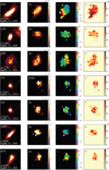 |
Fig. A.2 Same as Fig. A.1 for galaxies from MACS1206-08. |
| In the text | |
|
Fig. A.2 continued. |
| In the text | |
|
Fig. A.3 Observed velocity maps, velocity maps from the kinematic models, and rotation curves extracted on the major axis as indicated by the white solid lines on the maps. The blue circles and black solid line represent the curve extracted from the observed velocity maps and velocity maps from the model, respectively. The red dashed lines show the intrinsic rotation curves from the models. The vertical black solid lines indicate the value of the effective radius Re. The red circles and the horizontal black solid lines represent the velocity dispersion profile and the measured intrinsic velocity dispersion. The horizontal purple dashed lines indicate the intrinsic velocity dispersion obtained with GalPaK3D for five galaxies. |
| In the text | |
|
Fig. A.3 continued. |
| In the text | |
Current usage metrics show cumulative count of Article Views (full-text article views including HTML views, PDF and ePub downloads, according to the available data) and Abstracts Views on Vision4Press platform.
Data correspond to usage on the plateform after 2015. The current usage metrics is available 48-96 hours after online publication and is updated daily on week days.
Initial download of the metrics may take a while.