| Issue |
A&A
Volume 664, August 2022
|
|
|---|---|---|
| Article Number | A63 | |
| Number of page(s) | 19 | |
| Section | Extragalactic astronomy | |
| DOI | https://doi.org/10.1051/0004-6361/202142843 | |
| Published online | 04 August 2022 | |
Starbursts with suppressed velocity dispersion revealed in a forming cluster at z = 2.51
1
School of Astronomy and Space Science, Nanjing University, Nanjing, 210093, PR China
e-mail: This email address is being protected from spambots. You need JavaScript enabled to view it.
2
AIM, CEA, CNRS, Université Paris-Saclay, Université Paris Diderot, Sorbonne Paris Cité, 91191 Gif-sur-Yvette, France
3
Key Laboratory of Modern Astronomy and Astrophysics (Nanjing University), Ministry of Education, Nanjing 210093, PR China
e-mail: This email address is being protected from spambots. You need JavaScript enabled to view it.
4
National Astronomical Observatory of Japan, 2-21-1 Osawa, Mitaka, Tokyo 181-8588, Japan
5
Department of Astronomical Science, SOKENDAI (The Graduate University for Advanced Studies), Mitaka, Tokyo 181-8588, Japan
6
Aix Marseille Université, CNRS, LAM, Laboratoire d’Astrophysique de Marseille, Marseille, France
7
Cosmic Dawn Center (DAWN), Copenhagen, Denmark
8
DTU-Space, Technical University of Denmark, Elektrovej 327, 2800 Kgs. Lyngby, Denmark
9
Niels Bohr Institute, University of Copenhagen, Blegdamsvej 17, 2100 Copenhagen Ø, Denmark
10
Istituto Nazionale di Astrofisica, Vicolo dell’Osservatorio 5, 35122 Padova, Italy
11
Instituto de Física, Pontificia Universidad Católica de Valparaíso, Casilla 4059, Valparaíso, Chile
12
European Southern Observatory, Alonso de Córdova, 3107, Vitacura, Santiago 763-0355, Chile
13
Joint ALMA Observatory, Alonso de Córdova, 3107, Vitacura, Santiago 763-0355, Chile
14
Institute of Astronomy, Graduate School of Science, The University of Tokyo, 2-21-1 Osawa, Mitaka, Tokyo 181-0015, Japan
15
Astrophysics, Department of Physics, Keble Road, Oxford, OX1 3RH, UK
Received:
6
December
2021
Accepted:
9
May
2022
Abstract
One of the most prominent features of galaxy clusters is the presence of a dominant population of massive ellipticals in their cores. Stellar archaeology suggests that these gigantic beasts assembled most of their stars in the early Universe via starbursts. However, the role of dense environments and their detailed physical mechanisms in triggering starburst activities remain unknown. Here we report spatially resolved Atacama Large Millimeter/submillimeter Array (ALMA) observations of the CO J = 3−2 emission line, with a resolution of about 2.5 kpc, toward a forming galaxy cluster core with starburst galaxies at z = 2.51. In contrast to starburst galaxies in the field often associated with galaxy mergers or highly turbulent gaseous disks, our observations show that the two starbursts in the cluster exhibit dynamically cold (rotation-dominated) gas-rich disks. Their gas disks have extremely low velocity dispersion (σ0 ∼ 20−30 km s−1), which is three times lower than their field counterparts at similar redshifts. The high gas fraction and suppressed velocity dispersion yield gravitationally unstable gas disks, which enables highly efficient star formation. The suppressed velocity dispersion, likely induced by the accretion of corotating and coplanar cold gas, might serve as an essential avenue to trigger starbursts in massive halos at high redshifts.
Key words: galaxies: formation / galaxies: high-redshift / galaxies: clusters: general / galaxies: evolution / galaxies: ISM
© M.-Y. Xiao et al. 2022
 Open Access article, published by EDP Sciences, under the terms of the Creative Commons Attribution License (https://creativecommons.org/licenses/by/4.0), which permits unrestricted use, distribution, and reproduction in any medium, provided the original work is properly cited.
This article is published in open access under the Subscribe-to-Open model. This email address is being protected from spambots. You need JavaScript enabled to view it. to support open access publication.
1. Introduction
Galaxy clusters represent the densest environments and trace the most massive dark matter halos in the Universe (Kravtsov & Borgani 2012). It is well known that massive elliptical galaxies are enhanced in clusters (e.g., Dressler 1980; Peng et al. 2010). However, it remains unclear whether and how the dense environment affects their formation and quenching. To answer this question, we need to trace them back to the cosmic epoch when they are still actively forming stars.
During the last decade, a number of young clusters and protoclusters have been found at z > 2 (e.g., Wang et al. 2016; Casey 2016; Miller et al. 2018; Oteo et al. 2018), the peak of cosmic star formation history (Madau & Dickinson 2014). Contrary to mature clusters in the local Universe, which are dominated by massive quiescent galaxies in their cores (e.g., Dressler 1980), these young clusters and protoclusters host a significant population of massive star-forming galaxies. In particular, observations have revealed the ubiquity of starbursts in these high-z (proto)clusters. For example, Miller et al. (2018) observed a protocluster at z = 4.3 hosting at least 14 gas-rich galaxies in a projected region of 130 kpc in diameter with a total star formation rate (SFR) of 6000 M⊙ yr−1; Wang et al. (2016) identified an X-ray cluster at z = 2.51 with a SFR of about 3400 M⊙ yr−1 in the central 80 kpc region. Many observations have found starbursting overdensities in the early Universe (e.g., Blain et al. 2004; Casey et al. 2015; Casey 2016; Oteo et al. 2018), which are in line with the expectation of the hierarchical growth of structures associated with an enhancement of star formation or starburst galaxies in dense environments (Dannerbauer et al. 2014, 2017; Hayashi et al. 2016).
However, the triggering mechanism of high-z starbursts in dense environments is unclear. Observations have revealed evidence of merger and/or interactions in these starbursts in (proto)clusters (e.g., Coogan et al. 2018; Hodge et al. 2013), while simulations show the inefficiency of enhancing star formation in high-z galaxies, even in the event of the most drastic gas-rich major mergers (Fensch et al. 2017). Meanwhile, starburst galaxies in dense environments such as GN20, similar to those in the field, contain a rotating gas disk and do not exhibit major merger evidence (Hodge et al. 2012).
To understand the origin of starbursts in dense environments in the high-z Universe, spatially and spectroscopically resolved measurements of their gas kinematic are needed. However, the large cost of high-resolution and high-sensitivity observations of galaxies in the early Universe has always been a limitation for in-depth kinematic studies of high-z starbursts in (proto)clusters.
One of the most distant young clusters, CLJ1001 at zspec = 2.51 (Wang et al. 2016, W16, hereafter; see also Casey et al. 2015; Daddi et al. 2017; Wang et al. 2018; Cucciati et al. 2018; Gómez-Guijarro et al. 2019; Champagne et al. 2021), exhibits extended X-ray emission and encompasses an overdensity of massive star-forming galaxies, with a total SFR of ∼3400 M⊙ yr−1 in its 80 kpc core (the cluster virial radius is R200c ∼ 340 kpc) and a gas depletion time of ∼200 Myr. CLJ1001 is in the phase of rapid transformation from a protocluster to a mature cluster, which makes it an ideal laboratory to study the connection between the triggering mechanism of cluster starbursts and their dense environment. Revealing the physical origin of cluster starbursts is key to uncovering the formation and quenching mechanisms of massive galaxies in clusters, which has been a longstanding problem in extragalactic studies. With these aims, we have conducted high-resolution CO J = 3−2 emission line (CO(3−2), hereafter) observations with the Atacama Large Millimeter/submillimeter Array (ALMA) toward the cluster core of CLJ1001 (Fig. 1). Thanks to newly obtained ALMA high resolution data, in this paper we study the molecular gas spatial distribution and resolved kinematics of two massive starburst galaxies (SBs) and two star-forming main sequence galaxies (MSs) in the galaxy cluster CLJ1001.
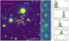 |
Fig. 1. Galaxy cluster CLJ1001 at z = 2.51 and the four member galaxies. Left: sky distributions of member galaxies around the cluster center. Red circles mark the two SBs and two MSs with the brightest CO(3−2) luminosities (S/N ≫ 10; S/N ∼ 30 for the two SBs) among all CO(3−2) detections (golden squares) in the central region of the cluster. The background is the Ks-band image from the UltraVista survey with a size of 70″ × 70″. The white cross shows the cluster center. The scale bar indicates half of the virial radius (R200c ∼ 340 kpc) of the cluster. The large green circle denotes the ALMA FOV, corresponding to FWHP ∼53″ of the ALMA antennas’ primary beam at 98.63 GHz. Middle: velocity-integrated intensity map (Moment 0) of CO(3−2) (golden contours) detected by ALMA overlaid on the HST/F160W image of the two SBs and two MSs. Each panel is 2.5″ × 2.5″. The angular resolution is 0.31″ × 0.25″ (gray-filled ellipse in the bottom-left corner). The contour levels start at ±3σ and increase in steps of ±3σ, where positive and negative contours are solid and dashed, respectively. The red cross in each panel denotes the centroid of the stellar emission determined from the HST/F160W image. The derived integrated fluxes are presented in Table 1. Right: CO(3−2) line spectra of the four member galaxies. The CO lines are binned at 90 km s−1, and the velocity range is shaded in green over which Moment 0 maps are integrated. The best-fit single Gaussian profiles are overlaid in red. |
This paper is organized as follows: in Sect. 2, we introduce the ALMA CO(3−2) line and 3.2 mm continuum observations. In Sect. 3, we study the two cluster SBs and two cluster MSs involved in this work and analyze the structural properties of their molecular gas, CO excitation, dust mass, molecular gas mass, and gas kinematics. In Sect. 4, we present the results focusing on their molecular gas kinematics and their gas disk stabilities. In Sect. 5, we discuss the triggering mechanism of the cluster SBs and the drivers of the low turbulent gas in the two cluster SBs. We summarize the main conclusions in Sect. 6.
We adopt a Chabrier (2003) initial mass function (IMF) to estimate the SFR and stellar mass. We assume cosmological parameters of H0 = 70 km s−1 Mpc−1, ΩM = 0.3, and ΩΛ = 0.7. When necessary, data from the literature have been converted with a conversion factor of SFR (Salpeter 1955, IMF) = 1.7× SFR (Chabrier 2003, IMF) and M* (Salpeter 1955, IMF) = 1.7 × M* (Chabrier 2003, IMF).
2. ALMA observations
We carried out observations of the CO(3−2) transitions at the rest-frame frequency of 345.796 GHz (98.630 GHz in the observed frame) for the galaxy cluster CLJ1001 at z = 2.51 with ALMA band-3 receivers. These ALMA Cycle 4 observations (Project ID: 2016.1.01155.S; PI: T. Wang) were taken between 2016 November and 2017 August with a total observing time, including calibration and overheads, of approximately 7 h. We adopted two different array configurations to obtain reliable measurements of total flux and resolved kinematics information: a more compact array configuration (C40-4) observing low-resolution large spatial scales, while a more extended array configuration (C40-7) observing high-resolution small spatial scales, with an on-source time of 1.6 h and 2.2 h, respectively. The observations were performed with a single pointing covering a field of view (FOV) of ∼53″, corresponding to the full-width at half power (FWHP) of the ALMA primary beam.
The calibration was performed using version 5.3.0 of the Common Astronomy Software Application package (CASA; McMullin et al. 2007) with a standard pipeline. We carried out the data reduction in two cases. Case 1 was designed to obtain a high-resolution cube of CO(3−2) line. To this end, we first combined two configurations’ data to form a single visibility table (UV table), using visibility weights of the compact configuration dataset (C40-4) to the extended configuration dataset (C40-7) proportional to 1:4. Imaging was carried out using the tclean task with 0.04″ pixels and a channel width of 30 km s−1 with a Briggs weighting of robust = 0.5 scheme. The resulting data cube has a synthesized beam size of 0.31″ × 0.25″ (∼2.5 kpc × 2.0 kpc in physical scale) with an rms sensitivity of ∼110−120 μJy beam−1 per channel at the phase center. Case 2 was designed to derive the total flux of our sources. To this end, we combined two configurations’ data with visibility weights proportional to 1:1. We used 0.2″ pixels and a channel width of 90 km s−1 with a uvtaper of 1″ and a natural weighting scheme for imaging. The natural weighting provides a better sensitivity, enabling us to measure the total flux more robustly. The resulting data cube has a synthesized beam size of 1.54″ × 1.37″ (∼12.3 kpc × 11.0 kpc in physical scale) and a central rms level of ∼60 μJy beam−1 per channel.
We also created the observed 3.2 mm continuum maps using Briggs weighting (robust = 0.5) after excluding the frequency range of the CO(3−2) line. We used the same method as for the CO(3−2) cubes to create two continuum maps with different angular resolutions. To estimate the continuum fluxes of our sources, we created continuum maps with a combination of two configurations’ data with visibility weights proportional to 1:1. The rms level is ∼4.3 μJy beam−1 in the map of 1.12″ × 1.06″ angular resolution (∼9.0 kpc × 8.5 kpc in physical scale). To measure the dust continuum sizes of our sources, we created continuum maps with a combination of two configurations’ data with visibility weights of the compact configuration dataset (C40-4) to the extended configuration dataset (C40-7) proportional to 1:4. The rms level is ∼6.9 μJy beam−1 in the map of 0.30″ × 0.24″ angular resolution (∼2.4 kpc × 1.9 kpc in physical scale).
Physical properties of the two SBs and two MSs in CLJ1001.
3. Data analysis
3.1. Starburst and main-sequence galaxies
Four member galaxies in the cluster CLJ1001 have a CO(3−2) line detected with high significances (35σ, 27σ, 23σ, and 10σ; see Table 1), allowing a detailed study of their kinematics. They are all massive star-forming galaxies with stellar masses of log(M*/M⊙)> 10.8, and they are located in the central 80 kpc region of the cluster (Fig. 1). These include two SBs and two MSs, with the SBs exhibiting specific star-formation rates (sSFR ≡ SFR/M*) more than three times the star-forming main-sequence (SFMS; Schreiber et al. 2015). According to their distances from the SFMS (ΔMS = SFR/SFRMS ∼ 5.8, 3.9, 0.7, and 0.7, where SFRMS is the SFR of a galaxy on the MS with the same stellar mass), the four galaxies were then named SB1, SB2, MS1, and MS2, respectively. The stellar masses were derived from spectral energy distribution (SED) fitting (W16; Wang et al. 2018, W18, hereafter). The SFRs were calculated from the infrared luminosity (Kennicutt & Evans 2012)1, which was derived from our infrared SED fitting (updated version of W16 and W18 with the addition of 3.2 mm data, see Sect. 3.4). The resulting SFRs of these four galaxies are consistent with those derived from the infrared luminosity of W16 and W18 within a 1σ confidence level. We note that all data presented here have been converted to a Chabrier (2003) IMF. The results are presented in Table 1.
The intense star formation of the two SBs shows that they are rapidly building up their stellar masses at a rate of 1314 ± 122 M⊙ yr−1 and 751 ± 338 M⊙ yr−1 (see Table 1). The CO(3−2) emission of all four galaxies reveals continuous velocity gradients in the observed gas rotation velocity fields (Moment 1) and position-velocity (PV) diagrams (Fig. 2). The observed velocity dispersion fields (Moment 2) exhibit central dispersion peaks. These are consistent with the kinematics of rotating disks.
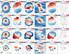 |
Fig. 2. CO morphology and kinematics of the four cluster members at z = 2.51. From left to right: ALMA maps (1.4″ × 1.4″) of velocity-integrated CO(1−0) flux (Moment 0), velocity field (Moment 1), velocity dispersion (Moment 2), position-velocity (PV) diagrams along the major axis, the best-fit Moment 1 model with GalPAK3D, and the residual between the data and the model. We note that these maps are without correction for beam-smearing. Gray-filled ellipses indicate the angular resolution of 0.31″ × 0.25″. The four member galaxies have regular rotating disks of molecular gas. |
3.2. Structural properties of the molecular gas
We measured the molecular gas structural properties of the four cluster members. To avoid uncertainties from the imaging process, we derived the source sizes with the visibility CO(3−2) data in the UV plane by fitting an elliptical Gaussian (task uvmodelfit). The best-fit semi-major and semi-minor axes for the SB1, SB2, MS1, and MS2 are shown in Table 1. As a comparison, we also performed a two-dimensional (2D) elliptical Gaussian fit on the high-resolution Moment 0 map of CO(3−2). The deconvolved semi-major and semi-minor axis values were broadly consistent with our UV analysis. We note that MS2 shows different sizes in the imaging and UV analyses, which could be caused by its lowest significance (10σ) of (3−2) detections among the four sources. The two SBs with higher significances of CO(3−2) detections than the two MSs show intrinsic sizes consistent in both methods within the error.
For the dust size, we only successfully measured the SB1 in the image plane, which has the highest signal-to-noise ratio (S/N ∼ 8) of 3.2 mm dust continuum emission among the four sources. The dust size of the SB1 was measured by a 2D elliptical Gaussian fit on the high-resolution Moment 0 map at 3.2 mm. We found that the dust size and molecular gas size of the SB1 are consistent within the error (see Table 1). Assuming a lack of significant size variation between the CO and dust continuum (e.g., Puglisi et al. 2019), we compared the molecular gas size (and/or dust size) of our sources with the literature. The typical dust size for galaxies at z = 2.5 with a stellar mass of 1010.9 M⊙ is 0.99 ± 0.34 kpc in radius from the GOODS-ALMA 1.1 mm survey (Fig. 15 in Gómez-Guijarro et al. 2022a). The dust distribution in the GOODS-ALMA sample was considered to be compact relative to the stellar distribution (van der Wel et al. 2014) in Gómez-Guijarro et al. (2022a). By further using the submillimeter compactness criterion (Puglisi et al. 2021), which is used to select compact galaxies, defined as a ratio of the stellar size (van der Wel et al. 2014) larger than the molecular gas size by a factor of 2.2, we conclude that the two SBs do not show compact gas disks.
3.3. CO excitation
The CO(3−2) line flux was measured from a 2D Gaussian fitting on the velocity-integrated intensity map (Moment 0) with the velocity range shown in Fig. 1. Then we calculated its luminosity  (Solomon & Vanden Bout 2005). The CO(1−0) line luminosity
  has already been obtained with the Karl G. Jansky Very Large Array (JVLA) observations in W18. Therefore, we can derive the CO excitation R31 with the CO(3−2) to CO(1−0) line luminosity ratio (
 ). The values are listed in Table 1. The R31 of the two SBs is around 0.8.
It has been shown that starburst galaxies generally have higher CO excitation rates relative to main-sequence objects (e.g., Valentino et al. 2020; Puglisi et al. 2021). However, there exists a large variation in the R31 values of high-z galaxies across the literature. In Riechers et al. (2020), the median R31 is 0.84 ± 0.26 for MS galaxies at z = 2−3 in the VLASPECS survey, while Daddi et al. (2015) showed an R31 of 0.42 ± 0.07 for MS galaxies at z ∼ 1.5, which is a factor of two smaller. In addition, Sharon et al. (2016) presented an R31 of 0.78 ± 0.27 for dusty submillimeter galaxies at z ∼ 2, while Harrington et al. (2018) reported an R31 of only 0.34 for the strongly lensed hyper-luminous infrared galaxies at z ∼ 1−3. For starburst galaxies in protoclusters at similar redshifts, they also exhibit a broad range of R31 ∼ 0.5−1.2 (e.g., HXMM20 at z = 2.6 in Gómez-Guijarro et al. 2019 and BOSS 1441 at z = 2.3 in Li et al. 2021). Therefore, the measured R31 values for the two SBs are consistent with a wide range of values observed in other galaxies (including MSs and starbursts) at similar redshifts (e.g., Boogaard et al. 2020; Aravena et al. 2014; Bothwell et al. 2013; Riechers et al. 2010). The higher-J CO transition observations (e.g., CO(5−4) and CO(6−5) probing warm and dense molecular gas) are necessary to establish whether the gas in the two SBs is highly excited as expected in starburst galaxies, or less excited as in MS galaxies.
3.4. Dust mass
To obtain the dust mass, Mdust, we performed the infrared SED fitting with CIGALE2 (Code Investigating Galaxies Emission; Burgarella et al. 2005; Noll et al. 2009; Boquien et al. 2019). We fit data from 24 μm up to the millimeter wavelengths (see the data at 24 μm, 100 μm, 160 μm, 870 μm, and 1.8 mm in W16, and the data at 3.2 mm in Table 1). The dust infrared emission model (Draine et al. 2014) combines two components with an extensive grid of parameters: the dust in the diffuse interstellar medium (ISM) heated by general diffuse starlight with a minimum radiation field Umin = 0.1−50 in the Habing unit (1.2 × 10⁻⁴ erg cm−2 s−1 sr−1; Habing 1968), and the dust tightly linked to star-forming regions illuminated by a variable radiation field (Umin < U < Umax) with a power-law distribution of a spectral index α = 1−3. The fraction of dust mass linked to the star-forming regions is γ = 0.0001−1. Among the two dust components, the mass fraction of dust in the form of the polycyclic aromatic hydrocarbons (PAH) is qPAH = 0.47−7.32%. We note that a large grid of models was generated by CIGALE and then fitted to the observations to estimate physical properties; for more details, readers can refer to Boquien et al. (2019). To investigate the active galactic nuclei (AGN) contributions to the infrared SEDs, we also fit the infrared SED with an additional AGN template (Fritz et al. 2006) using CIGALE. We did not find any sign of a significant contribution of an AGN (fAGN < 0.2%) in the infrared SEDs of our two SBs and two MSs, in agreement with previous literature constraints (W16,W18). The derived Mdust is given in Table 1. It is used to calculate the gas mass (in Sect. 3.5).
3.5. Molecular gas mass
We adopted three commonly used methods to obtain the total molecular gas mass, Mgas, and studied the gas properties of the two SBs and two MSs. The molecular gas masses were independently estimated based on the following: (i) the CO(1−0) line, (ii) the Mdust assuming a gas-to-dust mass ratio (δGDR), and (iii) the 3.2 mm dust continuum emission (see Table 2).
Gas properties of the two SBs and two MSs.
To obtain the total molecular gas mass Mgas, CO, we used the CO(1−0) luminosity (W18) instead of CO(3−2) to avoid uncertainties caused by the CO excitation ladder. The Mgas, CO was calculated by  , including a factor 1.36 correction for helium. As was done in our previous work (W18), the metallicity-dependent CO-to-H2 conversion factor, αCO(Z), was determined following Genzel et al. (2015) and Tacconi et al. (2018). The metallicity was derived from the stellar mass, using the mass-metallicity relation (Genzel et al. 2015).
The gas mass, Mgas, GDR, can also be determined through Mdust by employing the gas-to-dust ratio with a metallicity dependency (e.g., Magdis et al. 2011, 2012; Genzel et al. 2015; Béthermin et al. 2015). They assumed that the gas-to-dust ratio is only related to the gas-phase metallicity (δGDR − Z) following the relation of Leroy et al. (2011) 3:
 (1)
(1)
 (2)
(2)
The metallicity was determined from the redshift-dependent mass-metallicity relation (MZR; Genzel et al. 2015):
 (3)
(3)
where a = 8.74 and b = 10.4 + 4.46 log(1+z)−1.78 log(1+z)2. The metallicity derived here is on the PP04 scale (Pettini & Pagel 2004), consistent with the calibration used in Eq. (2) by Magdis et al. (2012). We adopted an uncertainty of 0.15 dex for the metallicities (Magdis et al. 2012).
The long-wavelength Rayleigh-Jeans (RJ) tail (≥ < SPSDOUBLEDOLLAR > ∼200 μm in the rest frame) of dust continuum emission is nearly always optically thin, providing a reliable probe of the total dust content. The RJ-tail method (Scoville et al. 2016) is based on an empirical calibration between the molecular gas content and the dust continuum at the rest frame 850μm, as the fiducial wavelength, which was obtained after considering a sample of low-redshift star-forming galaxies, ultra-luminous infrared galaxies, and z = 2−3 submillimeter galaxies. We used our single ALMA 3.2 mm measurement at the RJ tail to derive the total molecular gas mass, Mgas, 3.2 mm, following Eqs. (6) and (16) (corrected using the published erratum) in Scoville et al. (2016):
![Mathematical equation: $$ \begin{aligned} M_{\rm gas,3.2\,mm}&=1.78\, S_{\nu _{\rm obs}}\mathrm{[mJy]}\,(1+z)^{-(3+\beta )}\nonumber \\&\quad \times \left( \frac{\nu _{850\,\upmu \mathrm{m}}}{\nu _{\rm obs}}\right)^{2+\beta }\,(d_{L}[\mathrm{Gpc}])^2\,\,\,\,\,\,\,\,\,\,\nonumber \\&\quad \times \left\{ \frac{6.7\times 10^{19}}{\alpha _{\rm 850}} \right\} \, \frac{\Gamma _{0}}{\Gamma _{\rm RJ}}\, 10^{10}\,M_{\odot }\,\,\nonumber \\&\quad \mathrm{for} \, \, \lambda _{\rm rest} \gtrsim 250\, \upmu \mathrm{m}, \end{aligned} $$](/articles/aa/full_html/2022/08/aa42843-21/aa42843-21-eq29.gif) (4)
(4)
where Sνobs is the observed flux density at the observed frequency νobs corresponding to 3.2 mm, ν850 μm is the frequency corresponding to the rest-frame wavelength 850 μm, dL is the luminosity distance, and  . The dust emissivity power-law spectral index β is assumed to be 1.8. Furthermore, ΓRJ is a correction for the deviation of the Planck function from RJ in the rest frame given by
 (5)
(5)
and Γ0 = ΓRJ(Td, ν850, 0), where h is the Planck constant and k is the Boltzmann constant. The mass-weighted dust temperature Td is assumed to be 25 K, which is considered to be a representative value for both local star-forming galaxies and high-redshift galaxies (Scoville et al. 2016).
For our two SBs and two MSs, the Mgas, CO, Mgas, GDR, and Mgas, 3.2mm derived from three different methods are consistent with each other (within one sigma for the two SBs and within two sigma for the two MSs). All these values are presented in Table 2.
We note that in the empirical calibration of the RJ-tail method, αCO is set to 6.5 M⊙ (K km s−1 pc2) −1, which is different from what is used in our CO line method (αCO(Z)∼4 M⊙ (K km s−1 pc2) −1 in Table 2), both of which include a correction factor of 1.36 for helium. To keep the independent measurements of Mgas, 3.2mm and Mgas, CO and to maintain the consistency of the RJ-tail method commonly used in the literature, we did not perform any correction for αCO in the RJ-tail method.
We also note that the derived αCO(Z) in W18 is close to the Milky Way (MW) value (see Table 2). In general, two conversion factors are commonly used in the literature to convert CO luminosities into gas masses, that is to say the MW (αCO, MW = 4.36 M⊙(K km s−1 pc2)−1) and local starbursts (αCO, SB = 0.8 M⊙(K km s−1 pc2)−1; Downes & Solomon 1998; Tacconi et al. 2008) values. However, using αCO, SB = 0.8 M⊙(K km s−1 pc2)−1 for the two SBs would result in very low gas-to-dust ratios (δGDR ∼ 20), making the two SBs extreme cases. The resulting δGDR would be 4−5 times lower than the typical δGDR of solar-metallicity galaxies regardless of redshift (Rémy-Ruyer et al. 2014), which is more than three times lower than that of GN20 (δGDR ∼ 65 using αCO = 0.8; Magdis et al. 2011, 2012), and about three times lower than the median δGDR of local ultra-luminous infrared galaxies (Solomon et al. 1997; Downes & Solomon 1998). Therefore, we consider that using the derived αCO(Z) for the two SBs is more reasonable than using αCO, SB = 0.8 M⊙(K km s−1 pc2)−1. In addition, some high-z MS galaxies have been found to have gas properties of starbursts, the so-called SB in the MS, exhibiting compact dust structures (e.g., Elbaz et al. 2018; Gómez-Guijarro et al. 2022b). Similarly, distant starburst galaxies can also exhibit MW-like ISM conditions when they present extended, instead of compact star formation (e.g., Puglisi et al. 2021; Sharon et al. 2013) and/or large gas fractions. Here the two SBs exhibit both relatively extended CO sizes and large gas fractions (from the dust continuum and δGDR), favoring a MW-like αCO. Hence, these pieces of evidence are all consistent with our derived αCO(Z). We however show that even if we had chosen a local SB conversion factor (αCO, SB = 0.8 M⊙(K km s−1 pc2)−1) for the two SBs, the main conclusions of the paper would remain unchanged. We emphasize that for the two SBs, the gas masses derived with the three independent methods are consistent within a 1σ confidence level and the Mgas, GDR is independent of the assumption of the CO conversion factor.
It is worth mentioning that Gómez-Guijarro et al. (2019) also reported CO(1−0) luminosity values and Champagne et al. (2021) reported CO(1−0) luminosity and gas mass values for the two SBs and two MSs. We carefully compared our results with those derived using the CO(1−0) luminosity and/or gas mass from the above two papers, which mainly affect the gas fractions and Toomre Q values (Toomre 1964, described later in Sect. 4.2). We found that using the CO(1−0) luminosity (and gas mass) from different papers did not change our final results. They all agree with our results (gas fractions and Toomre Q values) within a 1σ confidence level. We emphasize again that in our work, the gas masses are calculated using three different methods that are consistent with each other (within 1σ confidence for the two SBs and within 2σ for the two MSs). In particular, for the gas mass derived from δGDR, it is independent of the CO(1−0) luminosity (and αCO), providing support to our results.
The derived molecular gas mass fractions, fgas = Mgas/(M* + Mgas), for the two SBs are ∼0.7 (0.70 and 0.66
 based on the CO emission line, 0.68
 and 0.65
 based on the δGDR, and 0.73
 and 0.61
 based on the 3.2 mm dust continuum emission for the SB1 and SB2, respectively). They are two times lower for the two MSs, fgas ∼ 0.3 (0.29
 and 0.25
 based on the CO emission line, 0.25
 and 0.15
 based on the δGDR, and 0.43
 and 0.18
 based on the 3.2 mm dust continuum emission for the MS1 and MS2, respectively). As a reference, the typical fgas of z = 2.5 SB and MS galaxies in the field with a stellar mass of 1011M⊙ is 0.7 and 0.5, respectively (Liu et al. 2019; Tacconi et al. 2018; Scoville et al. 2017). It shows that the two cluster SBs are gas-rich, similarly to field SBs.
3.6. Molecular gas kinematics
We investigated the kinematic properties of the molecular gas of the two cluster SBs and two cluster MSs by applying a three-dimensional (3D) kinematic modeling technique (GalPAK3D; Bouché et al. 2015) to the CO(3−2) line cube. The 3D kinematic modeling technique is currently the most advanced kinematic modeling approach for the low resolution observations (see e.g., Calistro Rivera et al. 2018; Fraternali et al. 2021; Tadaki et al. 2019; Fujimoto et al. 2021). GalPAK3D is a Bayesian parametric tool, using a Markov chain Monte Carlo (MCMC) approach to derive the intrinsic galaxy parameters and kinematic properties from a 3D data cube. The model is convolved with a 3D kernel to account for the instrument point spread function (PSF) and the line spread function (LSF) smearing effect. GalPAK3D can thus return intrinsic galaxy properties. We adopted a thick exponential-disk light profile and an arctan rotational velocity curve to fit the 0.3″ resolution cube in order to determine the maximum circular velocity Vmax and intrinsic velocity dispersion σ0. The arctan rotational velocity curve is Vrot ∝ Vmax arctan(r/rv), where rv is the turnover radius.
Figure 2 shows the best-fit models and residuals, based on the last 30% chain fraction with 20 000 iterations. For the two SBs and two MSs, our gas kinematic modeling provides a good description of the observed Moment 0, 1, and 2 maps (Figs. A.1–A.4). We also plotted the full MCMC chain from GalPAK3D for the two SBs and two MSs with 20,000 iterations to confirm the convergence of rotational velocity and intrinsic velocity dispersion (Fig. 3). The MCMC results of the fitting procedure are given in Figs. B.1–B.4, showing the posterior probability distributions of the model parameters and their marginalized distributions. The best-fitting values and their 1 σ uncertainties are summarized in Table 3.
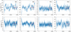 |
Fig. 3. Full MCMC chain for 20 000 iterations for the two SBs and two MSs. Each galaxy shows the fitting results of rotational velocity and intrinsic velocity dispersion. Red solid lines and black dashed lines refer to the median and the 1σ standard deviations of the last 30% of the MCMC chain. |
Summary of best-fit gas kinematic models for the two SBs and two MSs.
To investigate the performance of the fit, we compared the rotation velocity and velocity dispersion profiles from the observed data with that from the best-fit PSF-convolved model data. All values were derived from one-dimensional (1D) spectra extracted using circular apertures with diameters equal to an angular resolution of 0.31″ along the kinematic major axis. As shown in Fig. 4, the profiles from dynamical models and observations are consistent. Some points deviate from the models because of the flux contamination by neighboring sources. The derived best-fit σ0 from GalPAK3D is lower than the lowest observed velocity dispersion, which is reasonable because the latter is still affected by the beam-smearing effect even at the large radii probed by our observations
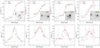 |
Fig. 4. Observations (points) and best-fit PSF-convolved models (blue lines) for rotation velocity and total velocity dispersion profiles along the kinematic major axis. Each point was extracted from the spectrum in an aperture whose diameter is equal to the angular resolution 0.31″ and the red one restricted to the spaxels with a S/N > 3 in the aperture. Orange and gray lines mark the intrinsic velocity dispersion σ0 and 1σ confidence from the GalPAK3D. The 3.5″ × 3.5″ HST/F160W images are shown in the bottom-right corner with the red crosses denote the corresponding source. Since SB2 and MS2 are close to each other with mixed fluxes, the points at the lowest radius of SB2 and the highest radius of MS2 are not fitted well with models. For MS1, the points at the lowest radius are not fitted well with models because of two neighboring sources at similar redshifts. The σ0 derived from GalPAK3D is lower than the lowest observed velocity dispersion profile because the latter one is still affected by the beam-smearing effect even at the large radii probed by our observations. |
Noticing that the best fit σ0 of SB1 is lower than the CO(3−2) channel width of 30 km s−1, we further tested the robustness of our fits. We applied the same analysis to the data cubes under the original channel width of ∼12 km s−1. The results were consistent with each other within errors. Therefore, considering that a better sensitivity can help detect fainter galaxy edges and better sample the flat part of the rotation curves, we have adopted the values from the data cubes with a channel width of 30 km s−1 in this work.
Finally, we made a simple simulation to test the robustness of σ0 and Vmax given by the kinematic model of GalPAK3D. Our purpose was to check first whether there is a global offset of the derived values or not, and second the reliability of the output uncertainties. To start, we randomly injected the best-fit PSF-convolved model data cube into the observed data cube (at the same positions as our galaxies, but at a different velocity and frequency to avoid the contamination of the CO emission from real sources). Then, we ran the GalPAK3D to derive σ0 and Vmax. These two steps were repeated 100 times for each galaxy. In the end, we obtained distributions of σ0 and Vmax. We calculated the median σ0 and uncertainty (16–84th percentile range) values for the SB1, SB2, MS1, and MS2, respectively. In general, there is no global offset of the derived values from the GalPAK3D, but the uncertainty is greatly underestimated by a factor of 5. Thus, we use the uncertainties of σ0 and Vmax given by this simulation in the main body of this paper, Figs. 5 and 6, and Table 3.
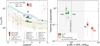 |
Fig. 5. Two cluster SBs have dynamically cold and gravitationally unstable gas disks. Left: ratio of the gas rotational to random motion (Vmax/σ0) as a function of redshift, with the comparison between the two cluster SBs and two cluster MSs and samples of observed and simulated field galaxies. The two cluster SBs and two cluster MSs are in red and green stars, respectively, with uncertainties derived from our simulation (see Sect. 3.6). Filled gray symbols with vertical bars show the median values and 16–84th percentile range of field star-forming galaxies, including molecular and ionized gas detections. When possible, we identified field starbursts (orange symbols) within these literature samples at z > 1 as galaxies with a SFR at least 0.5 dex higher than the SFMS. Blue triangles represent field starbursts with individual CO observations (Calistro Rivera et al. 2018; Barro et al. 2017; Swinbank et al. 2011; Tadaki et al. 2017, 2019). The faint red points show massive (M* > 1010 M⊙) rotation-dominated SBs at z > 4 which have been found recently (Rizzo et al. 2020, 2021; Lelli et al. 2021; Fraternali et al. 2021), but no information on their environment is available yet. The light-blue area shows Vmax/σ0 values for star-forming galaxies from Illustris-TNG50 simulations in the mass range 109–1011 M⊙ (Pillepich et al. 2019). The two lines with the light green and pink shaded regions describe Vmax/σ0 as a function of fgas and Toomre Q (Wisnioski et al. 2015), where a = |

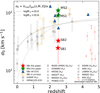 |
Fig. 6. Comparison of gas turbulence between the two cluster SBs and two cluster MSs and field galaxies. The intrinsic velocity dispersion increases with redshift. The symbol convention and the two lines are the same as in the left panel of Fig. 5. The two lines show the relation between the gas velocity dispersion, the gas fraction, and the disk instability for different stellar masses (Wisnioski et al. 2015). Here we assume Vmax = 130 km s−1, Q = 1, and |

4. Results
4.1. The two SBs have dynamically cold gas-rich disks with low velocity dispersions
Our SBs and MSs are located in a dense environment. To better understand the environmental effect on gas turbulence, we compare the four cluster members with field galaxies from the literature. The data included in Figs. 5 and 6 contain molecular and ionized gas observations. The ionized gas observations of the star-forming galaxies, sorted by redshifts from the lowest to the highest, are from surveys GHASP (log M*[M⊙]=9.4–11.0; log [M⊙]=10.6; Epinat et al. 2010), DYNAMO (log M*[M⊙]=9.0–11.8; log
 [M⊙]=10.3; Green et al. 2014), MUSE and KMOS (log M*[M⊙]=8.0-11.1; log
 [M⊙]=9.4, 9.8 at z ∼ 0.7, 1.3; Swinbank et al. 2017), KROSS (log M*[M⊙] = 8.7–11.0; log
 [M⊙]=9.9; Johnson et al. 2018), KMOS3D (log M*[M⊙]=9.0–11.7; log
 [M⊙]=10.5, 10.6, 10.7 at z ∼ 0.9, 1.5, 2.3; Wisnioski et al. 2015; Übler et al. 2019), MASSIV (log M*[M⊙]=9.4–11.0; log
 [M⊙]=10.2; Epinat et al. 2012), SIGMA (log M*[M⊙]=9.2–11.8; log
 [M⊙]=10.0; Simons et al. 2016), SINS (log M*[M⊙]=9.8–11.5; log
 [M⊙]=10.8; Förster Schreiber et al. 2009; Cresci et al. 2009), LAW09 (log M*[M⊙]=9.0–10.9; log
 [M⊙]=10.3; Law et al. 2009), AMAZE (log M*[M⊙]=9.2–10.6; log
 [M⊙]=10.0; Gnerucci et al. 2011), and KDS (log M*[M⊙]=9.0–10.5; log
 [M⊙]=9.8; Turner et al. 2017). The molecular gas observations of the star-forming galaxies, sorted by redshifts, are from the HERACLES survey (log M*[M⊙]=7.1–10.9; log
 [M⊙]=10.5; Leroy et al. 2008, 2009) and the PHIBSS survey (log M*[M⊙]=10.6-11.2; log
 [M⊙]=11.0; Tacconi et al. 2013). We note that although the velocity dispersion measured from the molecular gas is ∼10−15 km s−1 lower than from the ionized gas (with extra contributions from thermal broadening and expansion of the HII regions) in the local Universe, this difference becomes smaller with increasing redshift (Übler et al. 2019). Some field SBs with individual CO observations (Calistro Rivera et al. 2018; Barro et al. 2017; Swinbank et al. 2011; Tadaki et al. 2017, 2019) are indicated with blue triangles in Figs. 5 and 6. When possible, we also identified the field starbursts (orange symbols in Figs. 5 and 6) within the above star-forming samples, requiring their SFR to be at least 0.5 dex higher than the MS. In general, the gas in these field starbursts is slightly more turbulent than in main-sequence galaxies, showing a higher σ0, especially at 2 < z < 4. A similar trend of increasing σ0 as galaxies move above the MS at a fixed stellar mass is shown for star-forming galaxies at z = 0−3 (e.g., Perna et al. 2022; Wisnioski et al. 2015), suggesting that mergers or interactions would increase gas σ0 as they enhance star formation.
The gas disks of the two SBs are rotation-dominated with gas rotational to random motion ratios (Vmax/σ0) of 16.8 and 15.0
 , while the two MSs have a Vmax/σ0 of 3.6
 and 2.2
 (see Fig. 5 and Table 3). The Vmax/σ0 for the two SBs are more than three times higher than those for SBs and MSs in the field at the same epoch, either from observations or simulations. Moreover, they are as high as the median ratio for disk galaxies in the local Universe. As an example, the KMOS3D survey (Wisnioski et al. 2015) found a median Vmax/σ0 ≃ 3 (Vmax/σ0 ∼ 5 in Wisnioski et al. 2019) for field MS galaxies with stellar masses of ∼1010.5 M⊙ at z ∼ 2.3. From Illustris-TNG50 simulations (Pillepich et al. 2019), the typical star-forming galaxies in the stellar mass range 109 M⊙–1011 M⊙ have Vmax/σ0 ≃ 5 ± 1 at z = 2.5 (light-blue area in Fig. 5). In addition, using Vmax/σ0 ∝ 1/fgas(z, M*) (Wisnioski et al. 2015), we get a value of Vmax/σ0 ≃ 2 ± 1 at z = 2.5, which decreases with increasing redshift (gray lines; light-green and pink-shaded regions in Fig. 5).
We note that there has recently been some debate about potential observational effects (beam-smearing effect) on the dynamical state of (field) high-z galaxies (e.g., Di Teodoro et al. 2016; Kohandel et al. 2020). More specifically, when studying the gas kinematics with low spectral and spatial resolution data, the unresolved rotations within the PSF can artificially increase the value of σ0 and decrease the value of Vmax, leading to a severe systematic underestimation of the Vmax/σ0 ratio. The beam-smearing effect has been widely explored in local galaxies (e.g., see Fig. 6 in Di Teodoro & Fraternali 2015) and high-z simulated galaxies (e.g., Kohandel et al. 2020). Subsequently, given the high spatial and spectral resolution of ALMA observations, which have been able to reach subkpc spatial resolution in high-z galaxies, the beam-smearing effect is less significant. Compared to previous data, ALMA allows for a more robust way to measure intrinsic velocity dispersions. However, in our case, comparing two cluster SBs (with a spatial resolution of ∼0.3″ and a channel width of 30 km s−1) with other field SBs at similar redshifts and similar resolutions (with spatial resolutions of 0.1″–0.7″ and channel widths of 20–50 km s−1, except for one with a channel width of ∼100 km s−1), the σ0 values of the two cluster SBs are about three times lower than that of those field SBs (blue triangles in Fig. 6; Calistro Rivera et al. 2018; Barro et al. 2017; Swinbank et al. 2011; Tadaki et al. 2017). In addition, even at the same spatial and spectroscopical resolution, the σ0 values of the two cluster SBs are still more than three times lower than those of the two cluster MSs (green stars in Fig. 6). Furthermore, the simulations have confirmed the robustness of σ0 and Vmax for the two SBs and two MSs in our measurements (see Sect. 3.6). Therefore, we argue that the higher Vmax/σ0 and lower σ0 of the two cluster SBs with respect to field galaxies is a real physical difference, rather than being driven by observational effects.
In general, high-redshift star-forming galaxies are gas-rich and thus are believed to have a more turbulent ISM than local ones (Förster Schreiber & Wuyts 2020). While previous studies suggest that starburst galaxies are more likely associated with mergers or interactions, which are dynamically hot, the two cluster SBs surprisingly host dynamically cold disks, that is with a large Vmax/σ0. Recently, observations also found this type of phenomenon at z > 4 with the presence of massive (M* > 1010 M⊙) rotation-dominated SBs (faint red points in Fig. 5; Rizzo et al. 2020, 2021; Lelli et al. 2021; Fraternali et al. 2021), but no information on their environment is available yet.
The rotationally supported and dynamically cold disks of the two SBs imply low gas turbulent motions that are lower than for field SBs and MSs at the same redshift (Fig. 6). Hence, the two cluster SBs appear to be weakly affected by extreme internal and/or external physical processes, such as stellar or AGN feedback and galaxy mergers.
4.2. The two SBs have gravitationally unstable gas disks
To understand the triggering mechanism taking place in these two SBs, we further study the dynamical state of their disks. A rotating, symmetric gas disk is unstable with respect to the gravitational fragmentation if the Toomre Q parameter, Q = κσ0, gas/(πGΣgas) (Toomre 1964), is below a threshold value of Qcrit. The Qcrit = 1 is for a thin gas disk, and Qcrit = 0.67 for a thick gas disk. We calculated the gas surface density,  , where Mgas was derived from the CO(1−0) luminosity, the Mdust assuming a gas-to-dust mass ratio, and dust continuum emission at 3.2 mm. Here we adopt the maximum circular velocity Vmax, intrinsic velocity dispersion σ0, the disk half-light radius r1/2, and flat rotation curve with the epicyclic frequency
  (Binney & Tremaine 2008). All of these values were derived from the gas kinematic modeling.
The right panel of Fig. 5 shows the Q values of the two SBs and two MSs based on CO, δGDR, and dust continuum emission as a function of the main-sequence offset. For the two SBs and two MSs, the derived Q values decrease as the SFR offset to the SFMS increases. The two SBs present Q values much smaller than Qcrit. We note that using the local starbursts’ conversion factor (αCO, SB = 0.8 M⊙(K km s−1 pc2)−1) for the two SBs, the derived Toomre parameter Q values increase by a factor of five but still remain below Qcrit. The low Toomre Q means that the gas disk can easily collapse due to gravitational instabilities, leading to a starburst (see Sect. 5.1 for a more in-depth discussion). This is consistent with the fact that the SFE (1/tdep) values of the two SBs are ≫0.5 dex than the scaling relation of MS galaxies (Liu et al. 2019), suggesting that they have efficient star formation.
5. Discussion
5.1. Triggering mechanism of high-z cluster starburst
The dynamically cold, rotating gas disks of the two SBs are mainly due to a low level of gas turbulent motions. Their intrinsic velocity dispersions are extremely low, with σ0 ∼ 20−30 km s−1, while the two MSs have σ0 ∼ 90−110 km s−1 (see Table 3). Their σ0 values are about three times lower than that of field SBs at similar redshifts based on molecular gas observations from 2D and 3D kinematic modeling (blue triangles in Fig. 6; Calistro Rivera et al. 2018; Barro et al. 2017; Swinbank et al. 2011; Tadaki et al. 2017), and even field MS galaxies. We note that the σ0 values of the two cluster SBs are consistent with those of a group of massive (M* > 1010 M⊙) rotation-dominated SBs recently found at z > 4 (faint red points in Fig. 6; Rizzo et al. 2020, 2021; Lelli et al. 2021; Fraternali et al. 2021). In general, the gas in field SBs at z = 2−3 (blue and orange markers in Fig. 6) seems slightly more turbulent than that in field MSs, with a higher median σ0 by a factor of ∼1.5. Hence, the two cluster SBs exhibit strikingly different kinematic properties compared to field SBs at z ∼ 2.5, whether they are observed by molecular gas or ionized gas. These results challenge our current understanding of the physical origin of high-z starbursts in clusters and hint that mergers and interactions are not the only way to trigger starbursts.
In addition, in the study of gas disk stabilities (see Sect. 4.2 and Fig. 5), we find the two SBs have unstable gas disks, as shown by their relatively low Toomre Q values. This means that their gas disks can easily collapse due to gravitational instabilities. According to current theories of galaxy evolution, the self-regulated star formation of galaxies require marginally gravitationally unstable disks (Thompson et al. 2005; Cacciato et al. 2012). In short, the accretion of gas from the intergalactic medium to a gas disk increases the self-gravity of the gas disk. Once the self-gravity of the gas overcomes stellar radiation pressure, the gas disk becomes unstable and can easily collapse, triggering star-formation. As the stellar feedback injects energy into the ISM, thus increasing gas turbulence and radiation pressure, the gas disk then becomes stable. Subsequently, star formation becomes inefficient and the gas self-gravity dominates again. Therefore, the Toomre Q value of such a marginally unstable disk is always around Qcrit. However, in our case, the two SBs have much lower Toomre Q values than Qcrit and they have high gas fractions (∼0.7; see Table 2). The gas turbulence in these two SBs is very inefficient in balancing the gas self-gravity, leading to starbursts. In other words, in our work, the combination of the high gas fractions and the low velocity dispersions of the two SBs would naturally yield highly unstable gas disks, which in turn induce efficient starburst activities (Fig. 5). In fact, the two SBs have higher gas fractions than other MS galaxies, but they are still comparable to other SBs in the field (see Sect. 3.5). It is their low velocity dispersions that make the two cluster SBs unusual.
Thus, the most possible mechanism for inducing efficient star formation activity in the two cluster SBs is the self-gravitational instability of gas disks caused by the low σ0 (and the high gas fractions). In the following section, we discuss possible scenarios most likely to lead to the low σ0 and high gas fractions, which are believed to be the coplanar, corotating cold gas accretion through the cold cosmic-web streams.
5.2. Drivers of low turbulent gas in the two cluster SBs
We further explore the physical origin of the extremely low velocity dispersions and high gas fractions of the cluster SBs. The two primary energy sources of gas turbulence are stellar feedback and gravitational instability (Krumholz & Burkhart 2016; Krumholz et al. 2018), while a high gas fraction could either be due to a merger or gas infall (cold gas accretion). The two SBs favor a scenario in which cold gas is accreted via corotating and coplanar streams (e.g., Danovich et al. 2012, 2015). Indeed, in such a scenario, most of the gravitational energy is converted to rotation rather than dispersion, thus building up angular momentum (Kretschmer et al. 2020, 2021). As a result, the two cluster SBs would have high gas fractions, low turbulent gas disks with high rotational velocities (Vmax ∼ 400−500 km s−1; see Table 3), and relatively extended gas disk sizes. Simulations do predict a high occurrence rate of such configurations of corotating and coplanar cold gas accretion in massive galaxies and halos (Kretschmer et al. 2021; Dekel et al. 2020) for which galaxy merger events are rare enough to allow gas disks to survive over a long timescale. More specifically, the cold gas disk with Vmax/σ0 ≃ 5 in a z ∼ 3.5 galaxy, with a stellar mass of M* ∼ 1010 M⊙, typically survives for approximately five orbital periods (a duration time of ∼410 Myr) (Kretschmer et al. 2021), before being disrupted by a merger. Assuming the same duration time of 410 Myr between two merger events, we infer that our two cluster SBs, which have more massive cold gas disks with larger Vmax/σ0 > 10, would survive for ≳15 orbital periods to mergers.
Gas-rich major mergers can also lead to high gas fractions in the merger remnants. Numerical simulations and observations further indicate that rotating disks can reform rapidly after the final coalescence stage of the gas-rich mergers (e.g., Robertson et al. 2006; Hopkins et al. 2009; Ueda et al. 2014). However, simulations of gas-rich major mergers reveal enhanced gas turbulence and reduced sizes of disk components that survive or that one rebuilt after a merger (e.g., Bournaud et al. 2011), which conflicts with the observed low σ0 and relatively extended disk sizes of the two SBs. We highlight that the σ0 values of the two SBs are significantly lower than their field counterparts (not only field SBs, but also most field MSs). Meanwhile, we have not seen clear evidence of galaxy mergers in the two cluster SBs; this not only includes the CO(3−2) map, but also the high-resolution HST/F160W image tracing the stellar structures. While the possibility cannot be fully ruled out that the two SBs are in the final coalescence stage of gas-rich mergers, the chance that both SBs are caught in this short stage is small. Thus, the high gas fraction, low σ0, and lack of evidence for galaxy major mergers in the two SBs appear inconsistent with merger remnants.
In summary, the two cluster SBs have suppressed velocity dispersion and high gas fraction. These two unique properties of the two SBs support the scenario of corotating and coplanar cold gas accretion as the cause of their highly efficient star formation.
6. Conclusions
In this paper, we have studied the molecular gas kinematics of two SBs and two MSs in the most distant known X-ray cluster CLJ1001 at z = 2.51 (Fig. 1), based on ALMA high-resolution CO(3−2) observations (∼0.3″ corresponding to ∼2.5 kpc). These four galaxies show regular rotating gas disks, without clear evidence of a past gas-rich major merger (Fig. 2). While exploring the disk stabilities, we find strong evidence that the two cluster SBs have gravitationally unstable gas disks (right panel of Fig. 5). Therefore, we suggest that self-gravitational instability of the gas disks is the most likely mechanism that induces intense star formation in the two cluster SBs.
The two cluster SBs show dynamically cold gas-rich disks with significantly higher Vmax/σ0 than their field counterparts at similar redshifts, implying that their gas is low-turbulent (left panel of Figs. 5 and 6). The gas disks of the two cluster SBs have extremely low velocity dispersions (σ0 ∼ 20−30 km s−1), which are three times lower than their field counterparts at similar redshifts. The suppressed velocity dispersions (see Table 3) and high gas fractions (∼0.7; see Table 2) of the two cluster SBs yield gravitationally unstable gas disks, which enable highly efficient star formation. The unique properties of the two cluster SBs (high gas fraction and suppressed velocity dispersion) support the scenario in which corotating and coplanar cold gas accretion might serve as an essential avenue to trigger starbursts in forming galaxy clusters at high redshift. This may represent an important process other than mergers and interactions in triggering starbursts at high redshifts, at least in massive halos. Characterizing the environment of the recently found massive (M* > 1010 M⊙) rotation-dominated disks at z > 4 with suppressed velocity dispersion presents a unique opportunity to support this scenario further.
SFR = 1.49 × 10⁻¹⁰LIR in Kennicutt & Evans (2012), which uses a Kroupa 2001 IMF. Here we neglect the small differences between the Kroupa 2001 IMF and the Chabrier 2003 IMF, and assume the same SFRs derived based on the two IMFs.
CIGALE:https://cigale.lam.fr
Converted to the PP04 (Pettini & Pagel 2004) metallicity scale by Magdis et al. (2012).
Acknowledgments
We are very grateful to the anonymous referee for instructive comments, which helped to improve the overall quality and strengthened the analyses of this work. We thank Ken-ichi Tadaki and Nicolas Bouché for the helpful discussion of the molecular gas kinematics with GalPAK3D; Yong Shi, Alain Omont, Susan Kassin, Annagrazia Puglisi, Daizhong Liu, and Boris Sindhu Kalita for valuable discussions and suggestions that improved this paper. This paper makes use of the following ALMA data: ADS/JAO.ALMA #2016.1.01155.S. ALMA is a partnership of ESO (representing its member states), NSF (USA), and NINS (Japan), together with NRC (Canada), NSC, ASIAA (Taiwan), and KASI (Republic of Korea), in cooperation with the Republic of Chile. The Joint ALMA Observatory is operated by ESO, AUI/NRAO, and NAOJ. This work is supported by the National Key Research and Development Program of China (No. 2017YFA0402703), and by the National Natural Science Foundation of China (Key Project No. 11733002, Project No. 12173017, and Project No. 12141301). This work is also supported by the Programme National Cosmology et Galaxies (PNCG) of CNRS/INSU with INP and IN2P3, co-funded by CEA and CNES. M.-Y. X. acknowledges the support by China Scholarship Council (CSC). T.W. and K. K. acknowledges the support by NAOJ ALMA Scientific Research Grant Number 2017-06B. D. I. acknowledges the support by JSPS KAKENHI Grant Number JP21H01133.
References
- Aravena, M., Hodge, J. A., Wagg, J., et al. 2014, MNRAS, 442, 558 [Google Scholar]
- Barro, G., Kriek, M., Pérez-González, P. G., et al. 2017, ApJ, 851, L40 [NASA ADS] [CrossRef] [Google Scholar]
- Béthermin, M., Daddi, E., Magdis, G., et al. 2015, A&A, 573, A113 [Google Scholar]
- Binney, J., & Tremaine, S. 2008, in Galactic Dynamics: Second Edition, by James Binney and Scott Tremaine (Princeton, NJ USA: Princeton University Press) [CrossRef] [Google Scholar]
- Blain, A. W., Chapman, S. C., Smail, I., & Ivison, R. 2004, ApJ, 611, 725 [NASA ADS] [CrossRef] [Google Scholar]
- Boogaard, L. A., van der Werf, P., Weiss, A., et al. 2020, ApJ, 902, 109 [NASA ADS] [CrossRef] [Google Scholar]
- Boquien, M., Burgarella, D., Roehlly, Y., et al. 2019, A&A, 622, A103 [NASA ADS] [CrossRef] [EDP Sciences] [Google Scholar]
- Bothwell, M. S., Smail, I., Chapman, S. C., et al. 2013, MNRAS, 429, 3047 [Google Scholar]
- Bouché, N., Carfantan, H., Schroetter, I., et al. 2015, AJ, 150, 92 [CrossRef] [Google Scholar]
- Bournaud, F., Chapon, D., Teyssier, R., et al. 2011, ApJ, 730, 4 [NASA ADS] [CrossRef] [Google Scholar]
- Burgarella, D., Buat, V., & Iglesias-Páramo, J. 2005, MNRAS, 360, 1413 [NASA ADS] [CrossRef] [Google Scholar]
- Cacciato, M., Dekel, A., & Genel, S. 2012, MNRAS, 421, 818 [NASA ADS] [Google Scholar]
- Calistro Rivera, G., Hodge, J. A., Smail, I., et al. 2018, ApJ, 863, 56 [Google Scholar]
- Casey, C. M. 2016, ApJ, 824, 36 [CrossRef] [Google Scholar]
- Casey, C. M., Cooray, A., Capak, P., et al. 2015, ApJ, 808, L33 [NASA ADS] [CrossRef] [Google Scholar]
- Chabrier, G. 2003, PASP, 115, 763 [Google Scholar]
- Champagne, J. B., Casey, C. M., Zavala, J. A., et al. 2021, ApJ, 913, 110 [NASA ADS] [CrossRef] [Google Scholar]
- Coogan, R. T., Daddi, E., Sargent, M. T., et al. 2018, MNRAS, 479, 703 [NASA ADS] [Google Scholar]
- Cresci, G., Hicks, E. K. S., Genzel, R., et al. 2009, ApJ, 697, 115 [Google Scholar]
- Cucciati, O., Lemaux, B. C., Zamorani, G., et al. 2018, A&A, 619, A49 [NASA ADS] [CrossRef] [EDP Sciences] [Google Scholar]
- Daddi, E., Dannerbauer, H., Liu, D., et al. 2015, A&A, 577, A46 [NASA ADS] [CrossRef] [EDP Sciences] [Google Scholar]
- Daddi, E., Jin, S., Strazzullo, V., et al. 2017, ApJ, 846, L31 [Google Scholar]
- Dannerbauer, H., Kurk, J. D., De Breuck, C., et al. 2014, A&A, 570, A55 [NASA ADS] [CrossRef] [EDP Sciences] [Google Scholar]
- Dannerbauer, H., Lehnert, M. D., Emonts, B., et al. 2017, A&A, 608, A48 [NASA ADS] [CrossRef] [EDP Sciences] [Google Scholar]
- Danovich, M., Dekel, A., Hahn, O., et al. 2012, MNRAS, 422, 1732 [NASA ADS] [CrossRef] [Google Scholar]
- Danovich, M., Dekel, A., Hahn, O., et al. 2015, MNRAS, 449, 2087 [CrossRef] [Google Scholar]
- Dekel, A., Ginzburg, O., Jiang, F., et al. 2020, MNRAS, 493, 4126 [CrossRef] [Google Scholar]
- Di Teodoro, E. M., & Fraternali, F. 2015, MNRAS, 451, 3021 [Google Scholar]
- Di Teodoro, E. M., Fraternali, F., & Miller, S. H. 2016, A&A, 594, A77 [NASA ADS] [CrossRef] [EDP Sciences] [Google Scholar]
- Downes, D., & Solomon, P. M. 1998, ApJ, 507, 615 [NASA ADS] [CrossRef] [Google Scholar]
- Draine, B. T., Aniano, G., Krause, O., et al. 2014, ApJ, 780, 172 [Google Scholar]
- Dressler, A. 1980, ApJ, 236, 351 [Google Scholar]
- Elbaz, D., Leiton, R., Nagar, N., et al. 2018, A&A, 616, A110 [NASA ADS] [CrossRef] [EDP Sciences] [Google Scholar]
- Epinat, B., Amram, P., Balkowski, C., et al. 2010, MNRAS, 401, 2113 [Google Scholar]
- Epinat, B., Tasca, L., Amram, P., et al. 2012, A&A, 539, A92 [NASA ADS] [CrossRef] [EDP Sciences] [Google Scholar]
- Fensch, J., Renaud, F., Bournaud, F., et al. 2017, MNRAS, 465, 1934 [NASA ADS] [CrossRef] [Google Scholar]
- Fraternali, F., Karim, A., Magnelli, B., et al. 2021, A&A, 647, A194 [NASA ADS] [CrossRef] [EDP Sciences] [Google Scholar]
- Fritz, J., Franceschini, A., & Hatziminaoglou, E. 2006, MNRAS, 366, 767 [Google Scholar]
- Förster Schreiber, N. M., & Wuyts, S. 2020, ARA&A, 58, 661 [Google Scholar]
- Förster Schreiber, N. M., Genzel, R., Bouché, N., et al. 2009, ApJ, 706, 1364 [Google Scholar]
- Fujimoto, S., Oguri, M., Brammer, G., et al. 2021, ApJ, 911, 99 [Google Scholar]
- Genzel, R., Tacconi, L. J., Lutz, D., et al. 2015, ApJ, 800, 20 [Google Scholar]
- Gnerucci, A., Marconi, A., Cresci, G., et al. 2011, A&A, 528, A88 [NASA ADS] [CrossRef] [EDP Sciences] [Google Scholar]
- Green, A. W., Glazebrook, K., McGregor, P. J., et al. 2014, MNRAS, 437, 1070 [Google Scholar]
- Gómez-Guijarro, C., Riechers, D. A., Pavesi, R., et al. 2019, ApJ, 872, 117 [CrossRef] [Google Scholar]
- Gómez-Guijarro, C., Elbaz, D., Xiao, M., et al. 2022a, A&A, 658, A43 [NASA ADS] [CrossRef] [EDP Sciences] [Google Scholar]
- Gómez-Guijarro, C., Elbaz, D., Xiao, M., et al. 2022b, A&A, 659, A196 [NASA ADS] [CrossRef] [EDP Sciences] [Google Scholar]
- Habing, H. J. 1968, Bull. Astron. Inst. Netherlands, 19, 421 [Google Scholar]
- Harrington, K. C., Yun, M. S., Magnelli, B., et al. 2018, MNRAS, 474, 3866 [Google Scholar]
- Hayashi, M., Kodama, T., Tanaka, I., et al. 2016, ApJ, 826, L28 [CrossRef] [Google Scholar]
- Hodge, J. A., Carilli, C. L., Walter, F., et al. 2012, ApJ, 760, 11 [Google Scholar]
- Hodge, J. A., Carilli, C. L., Walter, F., et al. 2013, ApJ, 776, 22 [NASA ADS] [CrossRef] [Google Scholar]
- Hopkins, P. F., Cox, T. J., Younger, J. D., & Hernquist, L. 2009, ApJ, 691, 1168 [NASA ADS] [CrossRef] [Google Scholar]
- Johnson, H. L., Harrison, C. M., Swinbank, A. M., et al. 2018, MNRAS, 474, 5076 [NASA ADS] [CrossRef] [Google Scholar]
- Kennicutt, R. C., & Evans, N. J. 2012, ARA&A, 50, 531 [NASA ADS] [CrossRef] [Google Scholar]
- Kohandel, M., Pallottini, A., Ferrara, A., et al. 2020, MNRAS, 499, 1250 [Google Scholar]
- Kravtsov, A. V., & Borgani, S. 2012, ARA&A, 50, 353 [Google Scholar]
- Kretschmer, M., Agertz, O., & Teyssier, R. 2020, MNRAS, 497, 4346 [NASA ADS] [CrossRef] [Google Scholar]
- Kretschmer, M., Dekel, A., Freundlich, J., et al. 2021, MNRAS, 503, 5238 [NASA ADS] [CrossRef] [Google Scholar]
- Kroupa, P. 2001, MNRAS, 322, 231 [NASA ADS] [CrossRef] [Google Scholar]
- Krumholz, M. R., & Burkhart, B. 2016, MNRAS, 458, 1671 [NASA ADS] [CrossRef] [Google Scholar]
- Krumholz, M. R., Burkhart, B., Forbes, J. C., et al. 2018, MNRAS, 477, 2716 [Google Scholar]
- Law, D. R., Steidel, C. C., Erb, D. K., et al. 2009, ApJ, 697, 2057 [NASA ADS] [CrossRef] [Google Scholar]
- Lelli, F., Di Teodoro, E. M., Fraternali, F., et al. 2021, Science, 371, 713 [Google Scholar]
- Leroy, A. K., Walter, F., Brinks, E., et al. 2008, AJ, 136, 2782 [Google Scholar]
- Leroy, A. K., Walter, F., Bigiel, F., et al. 2009, AJ, 137, 4670 [Google Scholar]
- Leroy, A. K., Bolatto, A., Gordon, K., et al. 2011, ApJ, 737, 12 [Google Scholar]
- Li, Q., Wang, R., Dannerbauer, H., et al. 2021, ApJ, 922, 236 [NASA ADS] [CrossRef] [Google Scholar]
- Liu, D., Schinnerer, E., Groves, B., et al. 2019, ApJ, 887, 235 [Google Scholar]
- Madau, P., & Dickinson, M. 2014, ARA&A, 52, 415 [Google Scholar]
- Magdis, G. E., Daddi, E., Elbaz, D., et al. 2011, ApJ, 740, L15 [NASA ADS] [CrossRef] [Google Scholar]
- Magdis, G. E., Daddi, E., Béthermin, M., et al. 2012, ApJ, 760, 6\pg{\newpage} [NASA ADS] [CrossRef] [Google Scholar]
- McMullin, J. P., Waters, B., Schiebel, D., et al. 2007, Astronomical Data Analysis Software and Systems XVI, 376, 127 [NASA ADS] [Google Scholar]
- Miller, T. B., Chapman, S. C., Aravena, M., et al. 2018, Nature, 556, 469 [CrossRef] [Google Scholar]
- Muzzin, A., Marchesini, D., Stefanon, M., et al. 2013, ApJS, 206, 8 [Google Scholar]
- Noll, S., Burgarella, D., Giovannoli, E., et al. 2009, A&A, 507, 1793 [NASA ADS] [CrossRef] [EDP Sciences] [Google Scholar]
- Oteo, I., Ivison, R. J., Dunne, L., et al. 2018, ApJ, 856, 72 [Google Scholar]
- Peng, Y. J., Lilly, S. J., Kovač, K., et al. 2010, ApJ, 721, 193 [NASA ADS] [CrossRef] [Google Scholar]
- Perna, M., Arribas, S., Colina, L., et al. 2022, A&A, 662, A94 [NASA ADS] [CrossRef] [EDP Sciences] [Google Scholar]
- Pettini, M., & Pagel, B. E. J. 2004, MNRAS, 348, L59 [NASA ADS] [CrossRef] [Google Scholar]
- Pillepich, A., Nelson, D., Springel, V., et al. 2019, MNRAS, 490, 3196 [Google Scholar]
- Puglisi, A., Daddi, E., Liu, D., et al. 2019, ApJ, 877, L23 [Google Scholar]
- Puglisi, A., Daddi, E., Valentino, F., et al. 2021, MNRAS, 508, 5217 [NASA ADS] [CrossRef] [Google Scholar]
- Rémy-Ruyer, A., Madden, S. C., Galliano, F., et al. 2014, A&A, 563, A31 [Google Scholar]
- Riechers, D. A., Carilli, C. L., Walter, F., et al. 2010, ApJ, 724, L153 [NASA ADS] [CrossRef] [Google Scholar]
- Riechers, D. A., Boogaard, L. A., Decarli, R., et al. 2020, ApJ, 896, L21 [NASA ADS] [CrossRef] [Google Scholar]
- Rizzo, F., Vegetti, S., Powell, D., et al. 2020, Nature, 584, 201 [Google Scholar]
- Rizzo, F., Vegetti, S., Fraternali, F., et al. 2021, MNRAS, 507, 3952 [NASA ADS] [CrossRef] [Google Scholar]
- Robertson, B., Bullock, J. S., Cox, T. J., et al. 2006, ApJ, 645, 986 [NASA ADS] [CrossRef] [Google Scholar]
- Salpeter, E. E. 1955, ApJ, 121, 161 [Google Scholar]
- Schreiber, C., Pannella, M., Elbaz, D., et al. 2015, A&A, 575, A74 [NASA ADS] [CrossRef] [EDP Sciences] [Google Scholar]
- Scoville, N., Sheth, K., Aussel, H., et al. 2016, ApJ, 820, 83 [Google Scholar]
- Scoville, N., Lee, N., Vanden Bout, P., et al. 2017, ApJ, 837, 150 [Google Scholar]
- Sharon, C. E., Baker, A. J., Harris, A. I., et al. 2013, ApJ, 765, 6 [NASA ADS] [CrossRef] [Google Scholar]
- Sharon, C. E., Riechers, D. A., Hodge, J., et al. 2016, ApJ, 827, 18 [Google Scholar]
- Simons, R. C., Kassin, S. A., Trump, J. R., et al. 2016, ApJ, 830, 14 [Google Scholar]
- Solomon, P. M., & Vanden Bout, P. A. 2005, ARA&A, 43, 677 [NASA ADS] [CrossRef] [Google Scholar]
- Solomon, P. M., Downes, D., Radford, S. J. E., et al. 1997, ApJ, 478, 144 [NASA ADS] [CrossRef] [Google Scholar]
- Swinbank, A. M., Papadopoulos, P. P., Cox, P., et al. 2011, ApJ, 742, 11 [NASA ADS] [CrossRef] [Google Scholar]
- Swinbank, A. M., Harrison, C. M., Trayford, J., et al. 2017, MNRAS, 467,\pg{\break} 3140 [NASA ADS] [Google Scholar]
- Tacconi, L. J., Genzel, R., Smail, I., et al. 2008, ApJ, 680, 246 [Google Scholar]
- Tacconi, L. J., Neri, R., Genzel, R., et al. 2013, ApJ, 768, 74 [NASA ADS] [CrossRef] [Google Scholar]
- Tacconi, L. J., Genzel, R., Saintonge, A., et al. 2018, ApJ, 853, 179 [Google Scholar]
- Tadaki, K.-I., Kodama, T., Nelson, E. J., et al. 2017, ApJ, 841, L25 [NASA ADS] [CrossRef] [Google Scholar]
- Tadaki, K.-I., Iono, D., Hatsukade, B., et al. 2019, ApJ, 876, 1 [Google Scholar]
- Thompson, T. A., Quataert, E., & Murray, N. 2005, ApJ, 630, 167 [Google Scholar]
- Toomre, A. 1964, ApJ, 139, 1217 [Google Scholar]
- Turner, O. J., Cirasuolo, M., Harrison, C. M., et al. 2017, MNRAS, 471, 1280 [Google Scholar]
- Übler, H., Genzel, R., Wisnioski, E., et al. 2019, ApJ, 880, 48 [Google Scholar]
- Ueda, J., Iono, D., Yun, M. S., et al. 2014, ApJS, 214, 1 [Google Scholar]
- Valentino, F., Daddi, E., Puglisi, A., et al. 2020, A&A, 641, A155 [NASA ADS] [CrossRef] [EDP Sciences] [Google Scholar]
- van der Wel, A., Franx, M., van Dokkum, P. G., et al. 2014, ApJ, 788, 28 [Google Scholar]
- Wang, T., Elbaz, D., Daddi, E., et al. 2016, ApJ, 828, 56 [NASA ADS] [CrossRef] [Google Scholar]
- Wang, T., Elbaz, D., Daddi, E., et al. 2018, ApJ, 867, L29 [NASA ADS] [CrossRef] [Google Scholar]
- Wisnioski, E., Förster Schreiber, N. M., Wuyts, S., et al. 2015, ApJ, 799, 209 [Google Scholar]
- Wisnioski, E., Förster Schreiber, N. M., Fossati, M., et al. 2019, ApJ, 886,\pg{\break} 124 [Google Scholar]
Appendix A: Gas Kinematics: Comparison between the data and the best-fit model
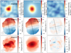 |
Fig. A.1. Comparison between the data and the best-fit model for the SB1. From top to bottom, this figure shows velocity-integrated CO(3−2) flux density (Moment 0), velocity field (Moment 1), and velocity dispersion (Moment 2) maps for the data (left panel); the best-fit model (middle panel); and the residual after subtracting the model from the data (right panel). Gray-filled ellipses in the bottom-left corner indicate the angular resolution of 0.31″ × 0.25″. Each panel is 1.4″ × 1.4″, with the north being up and the east to the left. |
Appendix B: Gas Kinematics: MCMC results
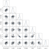 |
Fig. B.1. MCMC results for the SB1: the panels show the posterior probability distributions of seven model parameters using MCMC sampling with GalPAK3D. Their marginalized probability distribution are shown as histograms. The parameters are the total flux (Flux), the disk half-light radius (r1/2), the inclination angle (Incl.), the position angle (PA), the turnover radius (rv), the maximum circular velocity (Vmax), and the intrinsic velocity dispersion (σ0), in the same units as summarized in Table 3. The solid blue lines show median values. The black contour corresponds to the 68%, 95%, and 99.7% confidence intervals. |
All Tables
All Figures
|
Fig. 1. Galaxy cluster CLJ1001 at z = 2.51 and the four member galaxies. Left: sky distributions of member galaxies around the cluster center. Red circles mark the two SBs and two MSs with the brightest CO(3−2) luminosities (S/N ≫ 10; S/N ∼ 30 for the two SBs) among all CO(3−2) detections (golden squares) in the central region of the cluster. The background is the Ks-band image from the UltraVista survey with a size of 70″ × 70″. The white cross shows the cluster center. The scale bar indicates half of the virial radius (R200c ∼ 340 kpc) of the cluster. The large green circle denotes the ALMA FOV, corresponding to FWHP ∼53″ of the ALMA antennas’ primary beam at 98.63 GHz. Middle: velocity-integrated intensity map (Moment 0) of CO(3−2) (golden contours) detected by ALMA overlaid on the HST/F160W image of the two SBs and two MSs. Each panel is 2.5″ × 2.5″. The angular resolution is 0.31″ × 0.25″ (gray-filled ellipse in the bottom-left corner). The contour levels start at ±3σ and increase in steps of ±3σ, where positive and negative contours are solid and dashed, respectively. The red cross in each panel denotes the centroid of the stellar emission determined from the HST/F160W image. The derived integrated fluxes are presented in Table 1. Right: CO(3−2) line spectra of the four member galaxies. The CO lines are binned at 90 km s−1, and the velocity range is shaded in green over which Moment 0 maps are integrated. The best-fit single Gaussian profiles are overlaid in red. |
| In the text | |
|
Fig. 2. CO morphology and kinematics of the four cluster members at z = 2.51. From left to right: ALMA maps (1.4″ × 1.4″) of velocity-integrated CO(1−0) flux (Moment 0), velocity field (Moment 1), velocity dispersion (Moment 2), position-velocity (PV) diagrams along the major axis, the best-fit Moment 1 model with GalPAK3D, and the residual between the data and the model. We note that these maps are without correction for beam-smearing. Gray-filled ellipses indicate the angular resolution of 0.31″ × 0.25″. The four member galaxies have regular rotating disks of molecular gas. |
| In the text | |
|
Fig. 3. Full MCMC chain for 20 000 iterations for the two SBs and two MSs. Each galaxy shows the fitting results of rotational velocity and intrinsic velocity dispersion. Red solid lines and black dashed lines refer to the median and the 1σ standard deviations of the last 30% of the MCMC chain. |
| In the text | |
|
Fig. 4. Observations (points) and best-fit PSF-convolved models (blue lines) for rotation velocity and total velocity dispersion profiles along the kinematic major axis. Each point was extracted from the spectrum in an aperture whose diameter is equal to the angular resolution 0.31″ and the red one restricted to the spaxels with a S/N > 3 in the aperture. Orange and gray lines mark the intrinsic velocity dispersion σ0 and 1σ confidence from the GalPAK3D. The 3.5″ × 3.5″ HST/F160W images are shown in the bottom-right corner with the red crosses denote the corresponding source. Since SB2 and MS2 are close to each other with mixed fluxes, the points at the lowest radius of SB2 and the highest radius of MS2 are not fitted well with models. For MS1, the points at the lowest radius are not fitted well with models because of two neighboring sources at similar redshifts. The σ0 derived from GalPAK3D is lower than the lowest observed velocity dispersion profile because the latter one is still affected by the beam-smearing effect even at the large radii probed by our observations. |
| In the text | |
|
Fig. 5. Two cluster SBs have dynamically cold and gravitationally unstable gas disks. Left: ratio of the gas rotational to random motion (Vmax/σ0) as a function of redshift, with the comparison between the two cluster SBs and two cluster MSs and samples of observed and simulated field galaxies. The two cluster SBs and two cluster MSs are in red and green stars, respectively, with uncertainties derived from our simulation (see Sect. 3.6). Filled gray symbols with vertical bars show the median values and 16–84th percentile range of field star-forming galaxies, including molecular and ionized gas detections. When possible, we identified field starbursts (orange symbols) within these literature samples at z > 1 as galaxies with a SFR at least 0.5 dex higher than the SFMS. Blue triangles represent field starbursts with individual CO observations (Calistro Rivera et al. 2018; Barro et al. 2017; Swinbank et al. 2011; Tadaki et al. 2017, 2019). The faint red points show massive (M* > 1010 M⊙) rotation-dominated SBs at z > 4 which have been found recently (Rizzo et al. 2020, 2021; Lelli et al. 2021; Fraternali et al. 2021), but no information on their environment is available yet. The light-blue area shows Vmax/σ0 values for star-forming galaxies from Illustris-TNG50 simulations in the mass range 109–1011 M⊙ (Pillepich et al. 2019). The two lines with the light green and pink shaded regions describe Vmax/σ0 as a function of fgas and Toomre Q (Wisnioski et al. 2015), where a = |
| In the text | |
|
Fig. 6. Comparison of gas turbulence between the two cluster SBs and two cluster MSs and field galaxies. The intrinsic velocity dispersion increases with redshift. The symbol convention and the two lines are the same as in the left panel of Fig. 5. The two lines show the relation between the gas velocity dispersion, the gas fraction, and the disk instability for different stellar masses (Wisnioski et al. 2015). Here we assume Vmax = 130 km s−1, Q = 1, and |
| In the text | |
|
Fig. A.1. Comparison between the data and the best-fit model for the SB1. From top to bottom, this figure shows velocity-integrated CO(3−2) flux density (Moment 0), velocity field (Moment 1), and velocity dispersion (Moment 2) maps for the data (left panel); the best-fit model (middle panel); and the residual after subtracting the model from the data (right panel). Gray-filled ellipses in the bottom-left corner indicate the angular resolution of 0.31″ × 0.25″. Each panel is 1.4″ × 1.4″, with the north being up and the east to the left. |
| In the text | |
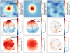 |
Fig. A.2. Same as Fig. A.1, but for the SB2. |
| In the text | |
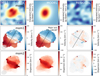 |
Fig. A.3. Same as Fig. A.1, but for the MS1. |
| In the text | |
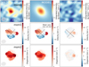 |
Fig. A.4. Same as Fig. A.1, but for the MS2. |
| In the text | |
|
Fig. B.1. MCMC results for the SB1: the panels show the posterior probability distributions of seven model parameters using MCMC sampling with GalPAK3D. Their marginalized probability distribution are shown as histograms. The parameters are the total flux (Flux), the disk half-light radius (r1/2), the inclination angle (Incl.), the position angle (PA), the turnover radius (rv), the maximum circular velocity (Vmax), and the intrinsic velocity dispersion (σ0), in the same units as summarized in Table 3. The solid blue lines show median values. The black contour corresponds to the 68%, 95%, and 99.7% confidence intervals. |
| In the text | |
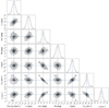 |
Fig. B.2. Same as Fig. B.1, but for the SB2. |
| In the text | |
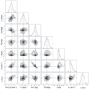 |
Fig. B.3. Same as Fig. B.1, but for the MS1. |
| In the text | |
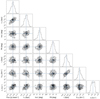 |
Fig. B.4. Same as Fig. B.1, but for the MS2. |
| In the text | |
Current usage metrics show cumulative count of Article Views (full-text article views including HTML views, PDF and ePub downloads, according to the available data) and Abstracts Views on Vision4Press platform.
Data correspond to usage on the plateform after 2015. The current usage metrics is available 48-96 hours after online publication and is updated daily on week days.
Initial download of the metrics may take a while.